Article

Selection and Location of Fixed-Step Capacitor Banks in Distribution Grids for Minimization of Annual Operating Costs: A Two-Stage Approach

by
Oscar Danilo Montoya
1,2,*,
Edwin Rivas-Trujillo
1 and
Diego Armando Giral-Ramírez
3
1
Grupo de Compatibilidad e Interferencia Electromágnetica, Facultad de Ingeniería, Universidad Distrital Francisco José de Caldas, Bogotá 110231, Colombia
2
Laboratorio Inteligente de Energía, Facultad de Ingeniería, Universidad Tecnológica de Bolívar, Cartagena 131001, Colombia
3
Facultad Tecnológica, Universidad Distrital Francisco José de Caldas, Bogotá 110231, Colombia
*
Author to whom correspondence should be addressed.
Computers 2022, 11(7), 105; https://doi.org/10.3390/computers11070105
Submission received: 19 April 2022 / Revised: 2 June 2022 / Accepted: 20 June 2022 / Published: 27 June 2022
(This article belongs to the Special Issue Computing, Electrical and Industrial Systems 2022)

Abstract

:
The problem regarding the optimal location and sizing of fixed-step capacitor banks in distribution networks with radial configuration is studied in this research by applying a two-stage optimization approach. The first stage consists of determining the nodes where the capacitor banks will be placed. In this stage, the exact mixed-integer nonlinear programming (MINLP) model that represents the studied problem is transformed into a mixed-integer quadratic convex (MIQC) model. The solution of the MIQC model ensures that the global optimum is reached given the convexity of the solution space for each combination of nodes where the capacitor banks will be installed. With the solution of the MIQC, the suitable nodes for the installation of the fixed-step capacitors are fixed, and their sizes are recursively evaluated in a power flow methodology that allows for determining the optimal sizes. In the second stage, the successive approximation power flow method is applied to determine the optimal sizes assigned to these compensation devices. Numerical results in three test feeders with 33, 69, and 85 buses demonstrate the effectiveness of the proposed two-stage solution method for two operation scenarios: (i) operation of the distribution system under peak load conditions throughout the year, and (ii) operation considering daily demand variations and renewable generation penetration. Comparative results with the GAMS software confirm the excellent results reached using the proposed optimization approach. All the simulations were carried out in the MATLAB programming environment, version 2021b, as well as using the Gurobi solver in the convex programming tool known as CVX.

1. Introduction

1.1. General Context

Electricity services have become public around the world, as they are considered necessary for social development in both rural and urban areas [1]. To provide electricity to all end users (industrial, residential, and commercial), distribution networks are used which are operated at medium- and low-voltage levels, most of which have radial structures [2]. Radial configuration means that a distribution grid composed of n nodes has n 1 lines, which allow for connecting all the end users to the substation by only one route [3,4]. Radial configurations are preferred in this context for two main reasons: (i) a radial configuration represents fewer kilometers in conductors and less electrical infrastructure (i.e., minimum investment costs) [5], and (ii) it reduces the complexity regarding the coordination issues of protective devices [6]. Even though these are strong, justifiable advantages for distribution companies, it is widely known that the radial configuration of the distribution networks increases the operating costs of the grid (i.e., the costs of the energy losses) in comparison with any weakly meshed distribution topology [7].

1.2. Motivation

Due to the increment in grid power and energy losses caused by the radial topology built into medium- and low-voltage distribution grids, distribution companies have implemented different alternatives to reduce their costs. These companies typically employ three main approaches to reduce grid power losses: (i) implementing grid reconfiguration schemes [8]; (ii) optimally siting and sizing dispersed generation and battery energy storage systems [9]; (iii) optimally siting and sizing reactive power compensators [7]. All of these methodologies can have positive impacts on the total grid power losses. However, in the case of the reconfiguration of distribution systems, it is necessary for distribution companies to construct new distribution lines (tie lines) in order to redefine the grid topology based on the current demand state of the network [10]. The installation of new lines may not be an economical task, and the reconfiguration problem is highly dependent on the demand behavior, which implies that an optimal solution for a particular load scenario may not be optimal for other load scenarios [11]. In the case of the optimal placement and sizing of dispersed generation and energy storage systems, the aforementioned devices can help with reducing energy losses in the distribution network [12]. However, their main application is in the reduction of the greenhouse gas emissions in rural areas, as well as that of energy purchasing costs at the substation bus. In addition, energy losses for these applications can sometimes increase, which are compensated by the use of renewables [13]. The main goal of installing renewable energy resources and batteries is minimizing the annual grid operating costs of the network, including investments and maintenance costs, where energy losses are typically not considered to be part of the objective function [14]. As for reactive power compensation, two main devices are used: (i) capacitor banks and (ii) distribution static compensators. The former are economical and have a long useful life as well as minimum maintenance requirements. The latter also have a long useful life, as well as the ability to dynamically compensate reactive power. However, they are more expensive in comparison with with capacitor banks, and they are less reliable, since these are composed of power electronic converters and require specialized control techniques and communication channels [15].
Considering the above, this research aims to propose a new optimization methodology that allows for minimizing the energy loss costs for distribution companies using fixed-step capacitor banks. Given that they are the most economical devices for reducing energy losses, they are well-recognized in the electrical sector, and they have long useful lives, regardless of the weather conditions, which implies that they can work correctly in areas with complex climatic conditions.

1.3. State of the Art

The problem concerning the optimal location and sizing of capacitor banks in electrical distribution networks is a well-known optimization problem for distribution grids. Here, we present a review of some contributions that employ metaheuristics and exact solution methods in order to deal with this optimization problem.
The authors of the ref. [16] suggested applying the simulated annealing algorithm to locate and size capacitor banks in radial distribution networks. The authors improved the effectiveness of the studied algorithm by using sensitivity factors in order to reduce the solution space, and their contribution was the inclusion of a duration curve for the system demand behavior. Numerical results in 9- and 69-node test feeders confirmed the applicability of the proposed methodology regarding the minimization of the objective function, which was associated with the annual energy losses and investment costs. The authors of the ref. [17] applied the flower pollination algorithm to locate and size capacitor banks in distribution networks while considering loss density factors in order to reduce the dimension of the solution space. The numerical results obtained from test feeders composed of 15, 69, and 118 nodes demonstrate the effectiveness of the proposed algorithms in comparison with literature reports based on metaheuristics. The authors focused on minimizing the annual grid operating costs while including the investment costs of the capacitor banks. However, only the peak load scenario was tested, which can oversize the capacitors when compared with daily load scenarios and also yield unrealistic reduction costs. The authors of the ref. [18] used the Chu and Beasley genetic algorithm to determine the location and size of fixed-step capacitor banks in distribution networks. The main contribution of this work has to do with the application of this methodology to radial and meshed distribution configurations without changing the power flow solver. Numerical results demonstrated the effectiveness of the proposed optimization approach when compared to the solution of the exact model in GAMS (general algebraic modeling system) and literature reports based on metaheuristics. The authors of the ref. [19] improved the flower pollination algorithm employed by [17] to allocate and size fixed-step capacitor banks in distribution grids. Computational validations in four test feeders composed of 33, 34, 69, and 85 buses demonstrated the effectiveness of this algorithm when compared to fuzzy logic and genetic algorithms. However, the authors only considered peak-load operation conditions, which, as previously mentioned, produces capacitor oversizing and unrealistic predictions regarding economic benefits.
The authors of the ref. [20] suggested the application of a discrete version of the vortex search algorithm to locate and size fixed-step capacitor banks in distribution grids with radial topology. Numerical results in the IEEE 33 and IEEE 69 grids demonstrate the effectiveness of this proposed algorithm in contrast with the flower pollination algorithm and the solution of the exact model in the GAMS software. The authors of the ref. [5] applied a specialized version of the genetic algorithm to locate and size capacitor banks, voltage regulators, and dispersed generators in distribution networks in order to reduce energy loss costs and improve voltage profiles across the distribution grid. Numerical results demonstrated the effectiveness of this version of the genetic algorithm in comparison with tabu search algorithms and particle swarm optimization methods. The authors of the ref. [21] proposed the application of the second-order cone programming with mixed-integer variables for siting and sizing fixed-step capacitor banks in radial distribution networks to reduce grid power losses under peak load conditions. Numerical simulations including annual grid operating costs under peak load conditions while considering investment costs in capacitor banks showed the effectiveness of the proposed methodology when compared to the exact solution in the GAMS software and some metaheuristic optimizers. The authors of the ref. [22] applied the classical genetic algorithm to locate and size capacitor banks in distribution networks. The main contribution of the authors corresponds to the usage of a real distribution network considering daily load and generation curves in order to ensure that the numerical results reached by the genetic algorithm reflected the operational reality of the network.
Additional solution methodologies to address the problem concerning the optimal location and sizing of capacitor banks in distribution grids are summarized in Table 1.
The most important characteristic of all the combinatorial optimization algorithms reported in Table 1 is that all of the algorithms work under a leader–follower concept (also known as the master–slave concept), where the leader algorithm is a heuristic or metaheuristic algorithm that defines the places or nodes where the capacitor banks will be installed, as well as their size. On the other hand, the follower corresponds to a power flow tool that allows for determining the final objective function values. The leader–follower optimization approach allows for decoupling the discrete optimization problem from that of the nonlinear power flow, which allows for exploring and exploiting the solution space through penalty factors, with excellent numerical results as reported in [32] for five different metaheuristic optimization methods compared regarding the problem of the optimal placement and sizing of capacitor banks for distribution system applications.
An additional characteristic of the methodologies listed in Table 1 is the use of objective functions related to power loss minimization, voltage profile improvements, and annual investment and operating cost minimization, which shows that, for distribution companies, the most important aspect when fixed-step capacitor banks are integrated into their grids corresponds to the economical feasibility of the final solution, including technical aspects that are economically quantifiable, as is the case for energy losses, as well as ensuring good voltage performances.

1.4. Contribution and Scope

Considering the most common aspects to be addressed regarding the problem of the optimal placement and sizing fixed-step capacitor banks in distribution networks, that is, annual investment and operating costs reduction and the use of master–slave optimization strategies, this research contributes with the following aspects:
  • It presents a two-stage optimization methodology to solve the studied problem, which separates the location problem from the power flow (sizing) problem. As for the location problem, this work proposes the use of a reduced mixed-integer quadratic convex (MIQC) formulation based on the optimal branch power flow formulation presented in [33]. This MIQC formulation allows for simplifying the exact MINLP model, and it defines the nodes for the installation of the fixed-step capacitor banks.
  • It determines the optimal sizes of the fixed-step capacitor banks in the slave stage by presenting a recursive-based power flow solution method that, once the nodes where the capacitor banks will be installed are defined, evaluates all the discrete possibilities for the capacitor sizes. The power flow tool used to evaluate the capacitor sizes corresponds to the triangular-based power flow method that is specialized for radial distribution system topologies [34].
It is worth mentioning that the MIQC part of the proposed two-stage optimization method has been previously proposed in [35] to address the problem concerning the optimal installation of solar photovoltaic generators. However, the recursive power flow solution to determine the optimal sizes of the capacitor banks has not been previously implemented. In addition, the proposed optimization method is only designed for strictly radial distribution networks due to the restrictions of the MIQC formulation regarding the branch convex power flow presented in [36].

1.5. Document Organization

The remainder of this work has the following structure: Section 2 presents the MIQC formulation to select the set of nodes where the fixed-step capacitor banks are to be installed; Section 3 shows the application of the recursive power flow solution method; Section 4 presents a summary of the proposed two-stage optimization methodology; Section 5 reveals the main characteristics of the test feeders, the daily load behavior, and the characterization of the objective function calculation; Section 6 presents the numerical results obtained with the proposed two-stage optimization approach and their comparison with literature reports; finally, Section 7 presents the conclusions drawn from this research.

2. Selection of the Nodes

This section presents the approximate mixed-integer quadratic convex (MIQC) model for the placement of the fixed-step capacitor banks. The MIQC model corresponds to the relaxation of the branch power flow model proposed in [33] to reconfigure radial distribution grids. The main characteristics of this formulation are as follows: (i) the voltage magnitudes are assumed close to the unity value in a per-unit representation, and (ii) active and reactive power losses in distribution lines can be neglected due to the fact that the power flows are larger in comparison. The approximated MIQC model to select the nodes where the capacitor banks will be assigned is defined in Equations (1)–(5) [37].
Objective function:
min z approx = C kWh T i j L h H R i j p i j , h 2 + q i j , h 2 Δ h + j N c C C c cap Q c x j c
Subject to:
p i j , h k : ( j k ) L p j k , h = P j , h d , j N , j slack , h H ,
q i j , h k : ( j k ) L q j k , h = Q j , h d c C Q c x j c , j N , j slack , h H ,
c C x j c 1 , j N , j slack ,
j N c C x j c N ava cap , j N , j slack .
where min z approx corresponds to the value of the objective function value containing the expected annual grid operating costs of the network, which combines the annual costs of the energy losses with the investment costs for the fixed-step capacitor banks; C kWh represents the expected average costs of the energy losses; T is the number of days in a year; R i j is the resistive parameter associated with the distribution line that connects node i with node j; p i j , h ( q i j , h ) corresponds to the active (reactive) power flow sent from nodes i to j for each period of time h; p j k , h and q j k , h represent the active and reactive power flows sent from node j to node k for the period of time h, respectively; P j , h d and Q j , h d are the active and reactive power demands at node j for each period of time h; C c cap represents the cost of a type c fixed-step capacitor bank; Q c represents the nominal reactive power rate of a type c fixed-step capacitor bank; x j c is the binary decision variable that defines whether the type c fixed-step capacitor bank is located at node j ( x j c = 1 ) or not ( x j c = 0 ); and N ava cap is an integer parameter that defines the number of fixed-step capacitor banks that can be added to the network. Note that N represents the set containing all the nodes of the network, and H is the set with all the periods of time included in the planning study.
The proposed MIQC model presented in Equations (1)–(5) can be interpreted as follows: Equation (1) presents an approximate objective function that evaluates the total investment costs of the fixed-step capacitor banks, with an estimation of the expected energy loss costs (note that the estimation of the power losses was initially introduced in [33]); Equations (2) and (3) represent the approximation of the active and reactive power flow variables in the system when it has been assumed that the voltages are ideal; inequality constraints (Equations (4) and (5)) define that it is only possible to locate a maximum of one fixed-step capacitor bank per node, and that the number of banks available for installation is a maximum of N ava cap .
Remark 1.
It is important to emphasize that the MIQC presented from Equation (1) to Equation (5) yields the set of nodes where the fixed-step capacitor banks will be installed, as well as their expected sizes [37]. However, the solution regarding the sizes corresponds to an approximate solution due to the simplification of the exact MINLP model. For this reason, these sizes are defined in the next step of the solution methodology through the recursive solution of multiple power flows for each fixed-step size combination.
On the other hand, it is worth mentioning that the proposed MIQC model defined in Equations (1)–(5) differs from the optimization model presented in [33] in two main respects: (i) our proposed model deals with reactive power compensation by means of the optimal installation of fixed-step capacitor banks in distribution networks while considering daily load curves, whereas the MIQC model in [33] was developed to solve the problem of optimal reconfiguration in radial distribution networks while considering the peak load operation scenario; and (ii) our optimization model is focused on the determination of the annual expected operating costs of the network, whereas the model proposed in [33] only focuses on the minimization of the power losses, without considering the intrinsic cost of opening and closing tie lines to reconfigure the distribution network.

3. Assigning the Optimal Sizes

This optimization stage aims to determine the optimal sizes of the fixed-step capacitor banks once the MIQC model has defined all the nodes where they are to be installed, i.e., the value of the variable x j c . To this effect, a recursive power flow solution approach is considered which is based on the well-known successive approximation method proposed by [38]. The recursive power flow approach evaluates each possible capacitor size available for the j nodes provided by the first optimization stage.
To illustrate the application of the recursive power flow formula to each possible capacitor size combination, the solution vector defined in Equation (6) is used.
y sol = [ i , j , k , | 3 , 9 , c ] ,
where y sol is the solution vector that determines the sizes of the capacitors placed in nodes i, j, and k. The most important characteristic of the solution vector in Equation (6) is that it allows for easily calculating the total investment costs of the fixed-step capacitor banks (see second component of the objective function defined in Equation (1)).
It is important to mention that, for the studied grids, the number of capacitors available for installations is three (i.e., N ava cap = 3 ), and the number of capacitor sizes available is 14 ( c = 14 ). This implies that the dimension of the solution space regarding the sizes of the capacitors is 14 3 , which corresponds to 2774 possible combinations [37]. Note that this dimension of the solution space is small, and it can be easily and exhaustively revised with the proposed recursive power flow evaluation method.
To evaluate each solution vector y sol , a new vector in the recursive power flow formulation is considered: S c a p , h . The purpose of S c a p , h is to add the sizes defined for the capacitor in the solution vector (see Equation (6) to the power flow problem. This vector is defined in Equation (7).
S i , h S j , h S k , h = j Q 3 j Q 9 j Q c ,
With the auxiliary vector defined in Equation (6), the successive approximation power flow formula proposed in [38] is modified, which takes the form presented in Equation (8).
V d , h m + 1 = Y d d 1 diag 1 V d , h m S c a p , h S d , h Y d s V s , h .
All of the components of the power flow Formula (8) can be consulted in [39].
Note that the selection of the successive approximation power flow method defined by Equation (8) is motivated by two main aspects: (i) its convergence can be ensured with the application of the Banach fixed-point theorem [40]; and (ii) it can be used for radial and meshed distribution networks with no changes to its formulation [39]. The second aspect is very important since it allows for extending the proposed two-stage solution methodology to meshed configurations with no change regarding the radial operation scenario.
To define the stopping criterion of the recursive power flow Formula (8), the difference between two consecutive solutions at the iterations m and m + 1 is used. This stopping criterion is defined in Equation (9).
max h | | V d , h m + 1 | | V d , h m | | ε ,
where ε is the tolerance value, which is assigned as 1 × 10 10 , as recommended in [38].
Now, with the solution of the power flow problem through the application of Equation (8), the total grid power losses of the network can be calculated for each period of time, as defined in Equation (10):
P loss , h = real V h Y bus V h ,
where V h is the vector containing the substation and demand voltages ordered as [ V s , h V d , h ] , and Y bus is the distribution network’s nodal admittance matrix. With the power losses for each period of time, the exact operating costs of the distribution systems with fixed-step capacitor banks, that is, min z cos ts , can obtained as defined in Equation (11).
min z cos ts = C kWh T i j L h H P loss , h Δ h + j N c C C c cap Q c x j c

4. Summary of the Solution Methodology

The two-stage solution methodology proposed in this research for locating and sizing fixed-step capacitor banks in radial distribution networks is summarized in Algorithm 1.
Algorithm 1: Solution methodology to locate and size fixed-step capacitor banks in distribution grids.
Computers 11 00105 i001

5. Test Feeder Information

With the purpose of validating the proposed hybrid mathematical formulation, three test feeders broadly used in the current literature are considered. These are the IEEE 33, IEEE 69, and IEEE 85 systems. The parametric information for these grids is presented below. Note that, with the first two test feeders, the application of the proposed optimization method with respect to the literature on peak load operation scenarios is validated. The third test feeder is used to validate the proposed multi-period planning scenario.

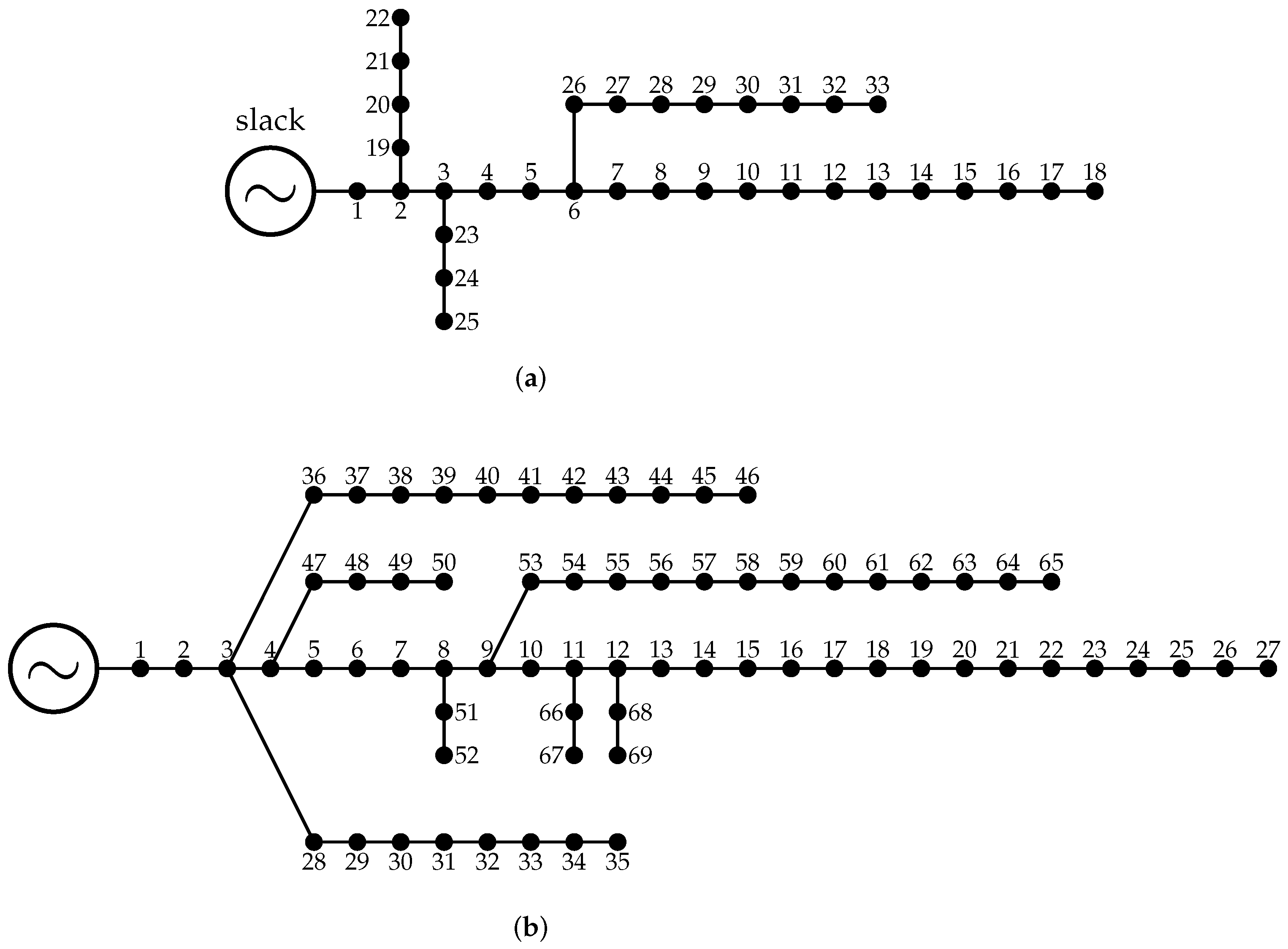
5.1. IEEE 33-Bus Grid

The IEEE 33-bus grid is an electrical network that operates with 12.66 kV at the substation bus located at node 1. This system has a radial structure, that is, 33 buses and 32 lines. The electrical configuration of this test feeder is shown in Figure 1a and its electrical parameters in Table 2.

5.2. IEEE 69-Bus Grid

The IEEE 69-bus grid is an electrical network that operates with 12.66 kV at the substation bus located at node 1. This system is radial, that is, it has 69 buses and 68 lines. The electrical configuration of this test feeder is shown in Figure 1b and its electrical parameters in Table 3.

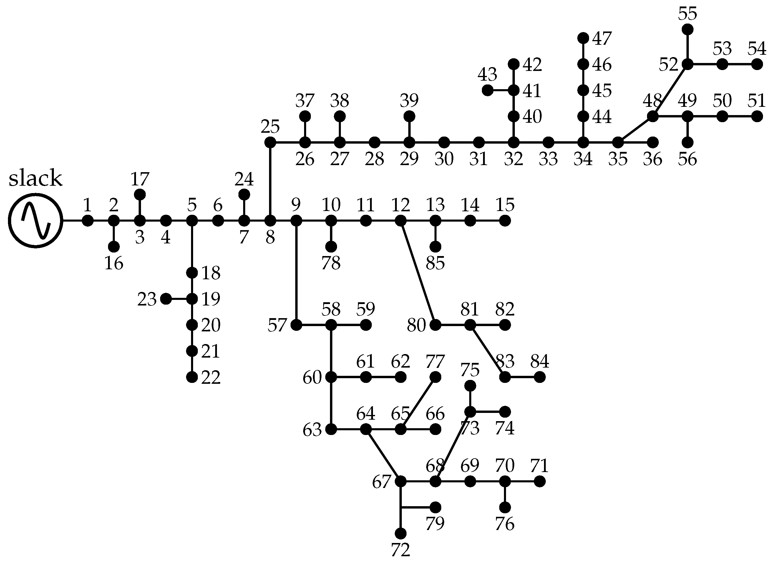
5.3. IEEE 85-Bus Grid

The IEEE 85-bus grid is a medium-voltage distribution grid comprising 85 nodes and 84 distribution lines (with a radial structure) operated with 11 kV as the substation voltage connected at node 1 (see Figure 2).
The total active and reactive power consumption of this system is 2570.28 + j 2622.20 kVA under peak load conditions [41]. The electrical information regarding branch impedances and nodal loads is presented in Table 4.

5.4. Economic Assessment Parameters

To determine the annual grid’s operating costs when fixed-step capacitor banks are installed, the information on their sizes and costs is shown in Table 5 (adapted from [19]).

6. Computational Implementation

The proposed two-stage optimization approach was implemented in version 2019b of the MATLAB software. The mixed-integer linear programming model was implemented using CVX and the Gurobi solver. The recursive power flow solution was implemented by means of our own scripts using the successive approximation power flow formulation. All simulations were run on a desktop computer with an INTEL(R) Core(TM) i 7 7700 2.8 -GHz CPU and 16.0 GB of RAM on a 64-bit version of Microsoft Windows 10. In the case of the GAMS software, version 23.5 was used along with the BONMIN solver [42].
Note that, in order to calculate the percentage of improvement of the proposed two-stage optimization methodology with respect to the benchmark cases, the following expression was used:
Imp % = 100 % | z cos t bc | | z cos t | z cos t bc
where Imp % represents the percentage of improvement with respect to the benchmark case, and z cost bc is the operating cost of the network with no fixed-step capacitor banks installed (that is, benchmark simulation case).

6.1. Comparison with Literature Reports

To demonstrate that the proposed two-stage solution methodology is efficient in determining the optimal siting of the fixed-step capacitor banks in radial distribution networks, here, our approach is compared with four different optimization methods reported in the current literature when the objective function is to minimize the total grid power losses (see Table 6). These methods are: the analytical method (AM) [43], the two-stage method (TSM), the hybrid fuzzy-based genetic algorithm (FRCGA) [44], GAMS [18], teaching-learning based optimization [45], and the flower pollination algorithm (FPA) [19].
Numerical results in Table 6 show that the proposed two-stage optimization method addresses the problem of the optimal location and sizing of fixed-step capacitor banks in distribution systems with a high efficiency when compared with the literature reports. Note that for both test feeders, the final location and sizes for the reactive power compensators reached with the MIQC model allow for better objective function vales when compared with the best report in [19]. In the case of the IEEE 33-bus grid, the proposed MIQC model reaches an objective function of 138.473 kW, which is 0.6020 kW better than the FPA, whereas in the IEEE 69-bus grid, this improvement is about 0.1880 kW with respect to the GAMS solution. Even though if this results represent small improvements with respect to the literature reports, these confirm the effectiveness of the proposed model in dealing with the minimization of the annual grid operating costs including fixed-step capacitor banks into distribution networks with a radial configuration.

6.2. IEEE 33-Bus Grid

Regarding the IEEE 33-bus grid, it was considered that the system was operated under the peak load conditions throughout the year, as recommended in [19]. The proposed MIQC model determined that the fixed-step capacitor banks should be located at nodes 13, 24, and 30. Once these placements were fixed, in the second optimization stage, the recursive power flow evaluation defined that the optimal sizes for the fixed-step capacitor banks were 450, 450, and 1050 kvar, respectively. Note that, if this solution is implemented, then the expected reduction compared to the benchmark case (USD/year 35,445.909) is about USD/year 11, 698.592, i.e., 33.04%. It is important to mention that, in order to reach this solution in the IEEE 33-bus grid, it is only necessary to invest USD/year 467.10 in reactive power compensators. To demonstrate the effectiveness of the proposed MIQC model, Table 7 is presents the comparison between the first three solutions reached by our two-stage solution proposal and the optimal solution found via the exact model in GAMS. Note that the solution reached using the proposed two-stage optimization method reduces the GAMS solution by about USD/year 111.9960, that is, 0.47 % of improvement of the MIQC model in comparison with the GAMS solution.
The most interesting result in Table 7 is that, with slight modifications in the sizes of the capacitor banks at nodes 24 and 30 (variations of 150 kvar), solutions are found with just 10 dollars of difference, all of them better than the solution found with GAMS.
One of the main results in Table 7 is that, with the proposed two-stage optimization method, it is possible to list the alternative solutions. Note that, in this list, there are three solutions with better final values regarding the final objective function than in the solution yielded by GAMS.

6.3. IEEE 69-Bus Grid

In this test feeder, and considering a peak-load operation scenario as reported in [19], the solution of the MIQC model in the nodal selection stage identified nodes 11, 21, and 61 as the optimal places to locate fixed-step capacitor banks. By fixing these nodal placements for the capacitors, in the refinement stage, the sizes found for the capacitors were 450, 150, and 1200 kvar, respectively. With this solution, the yearly operating cost reduction compared to the benchmark case (USD/year 37,812.056) is about USD/year 12,966.81, i.e., 34.29%. Note that this solution only requires an investment of USD/year 392.85 by the distribution company. On the other hand, Table 8 presents the comparisons between the solution reached using the GAMS software (exact MINLP solution) and the first four solutions found using the proposed two-stage solution approach. Note that the solution reached using the proposed two-stage optimization method reduces the GAMS solution by about USD/year 31.6640, i.e., 0.13 % of improvement of the MIQC model with respect to the GAMS solution.
The results in Table 8 show that the proposed two-stage optimization approach provides at least four solution methods with better numerical performance with respect to the objective function when compared to the GAMS solution. In addition, as with the IEEE 33-bus feeder, for this test system, it is observed that small variations (150 kvar) in some nodes yield solutions with expected reductions lower than 31 dollars per year of operation.

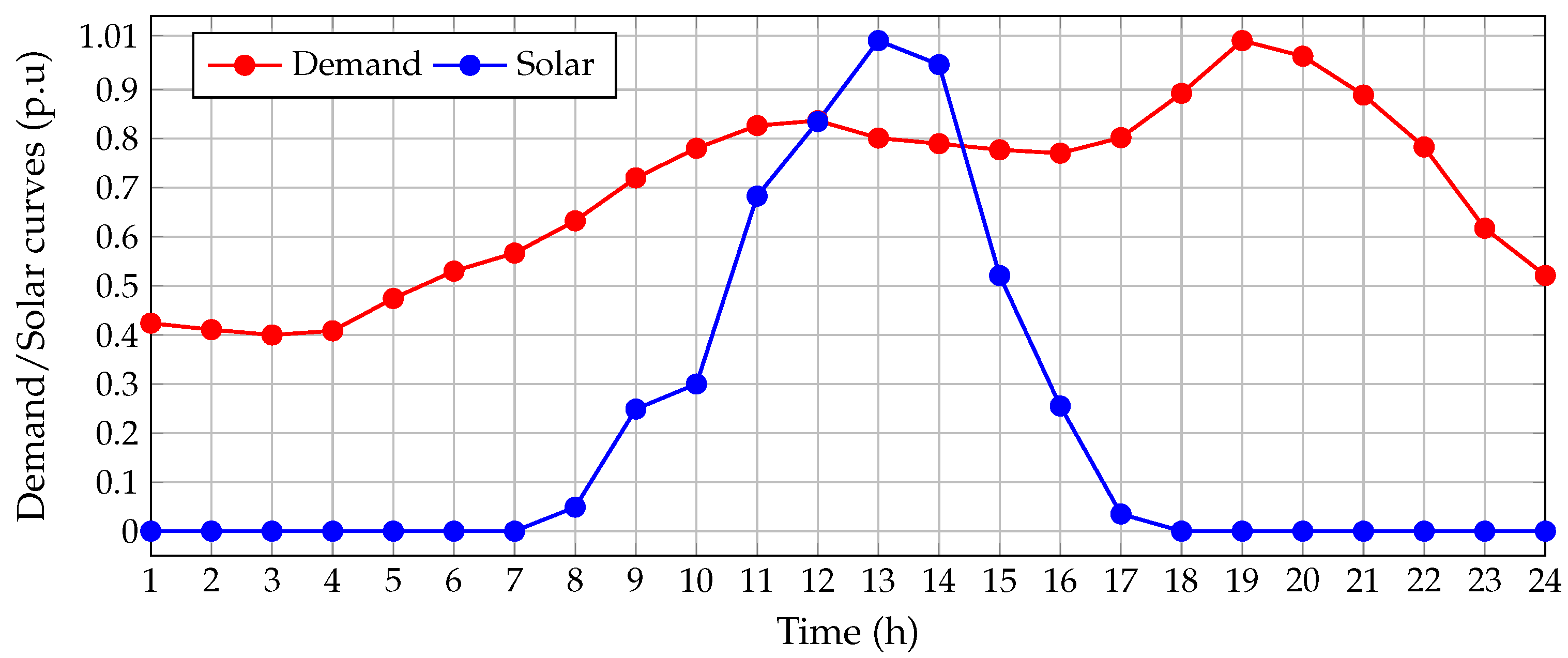
6.4. Numerical Results Considering Daily Load Variations

This subsection extends the analysis of the optimal placement of the fixed-step capacitor banks to daily operation scenarios while considering the presence of solar photovoltaic (PV) generation and daily load variations [13]. The demand load variations and the expected solar PV generation are depicted in Figure 3.
In the case of PV generation, the optimal sizes reported in [13] for the IEEE 85-bus test feeder are considered. These PV sources are located in nodes 35, 67, and 71, with sizes of 1631.31, 463.33, and 503.80 kW, respectively.
In addition, two simulation scenarios are considered. The first case involves the operation of the IEEE 85-bus grid while only considering the daily power demand with zero penetration of PV sources. The second case includes both curves, taking into account that the PV sources generate the maximum power available all the time.

6.4.1. Daily Operation without PV Generation

In this simulation case, the expected annual operating costs of the network without including fixed-step capacitor banks (i.e., the benchmark case) were USD/year 27,924.793. Once the two-stage optimization methodology was applied to the IEEE 85-bus grid, the nodes found for placing the fixed-step capacitor banks were 9, 34, and 67. With these locations, the annual expected operating costs of the network considering daily load variation were reduced to USD/year 16,089.331, i.e., a reduction of 42.38%. The sizes of the capacitors were 600, 450, and 450 kvar, respectively, with an annual investment of 359.70 dollars. Figure 4 presents the daily behavior of the energy losses for one day in this simulation scenario.
As expected, the results in Figure 4 show that the daily energy losses are reduced when the capacitor banks are installed in the distribution grid. For this simulation scenario, the daily energy losses are 3989.256 kWh/day when no capacitor banks are installed, and these are reduced to 2247.090 kWh/day.

6.4.2. Daily Operation including PV Generation

In this simulation scenario, the optimal location of fixed-step capacitor banks is evaluated while considering the PV generators to be active and with maximum power generation. The annual expected operating costs without integrating capacitor banks (i.e., the benchmark case) was USD/year 21,313.872. On the other hand, when the MIQC model was solved, the nodes where the fixed-step capacitor banks were to be placed were 9, 34, and 67 (note that these are the same nodes for the previous simulation scenario). Now, fixing these nodes in the recursive power flow approach, the optimal sizes for these capacitors were 600, 450, and 450 kvar (these sizes are also the same as those reached in the previous simulation scenario). With these sizes, the expected annual grid operating costs of the network are reduced to USD/year 10,574.253, that is, a 50.39% reduction compared to the benchmark case. Note that, in order to reach this solution, the total investment in fixed-step capacitor banks is 359.70 dollars. Figure 5 presents the daily behavior of the energy losses for one day in this simulation scenario.
As expected, the results in Figure 5 show that the daily energy losses are reduced when the capacitor banks are installed in the distribution grid. For this simulation scenario, the daily energy losses are 3044.839 kWh/day when no capacitor banks are installed, and these are reduced to 1459.222 kWh/day.

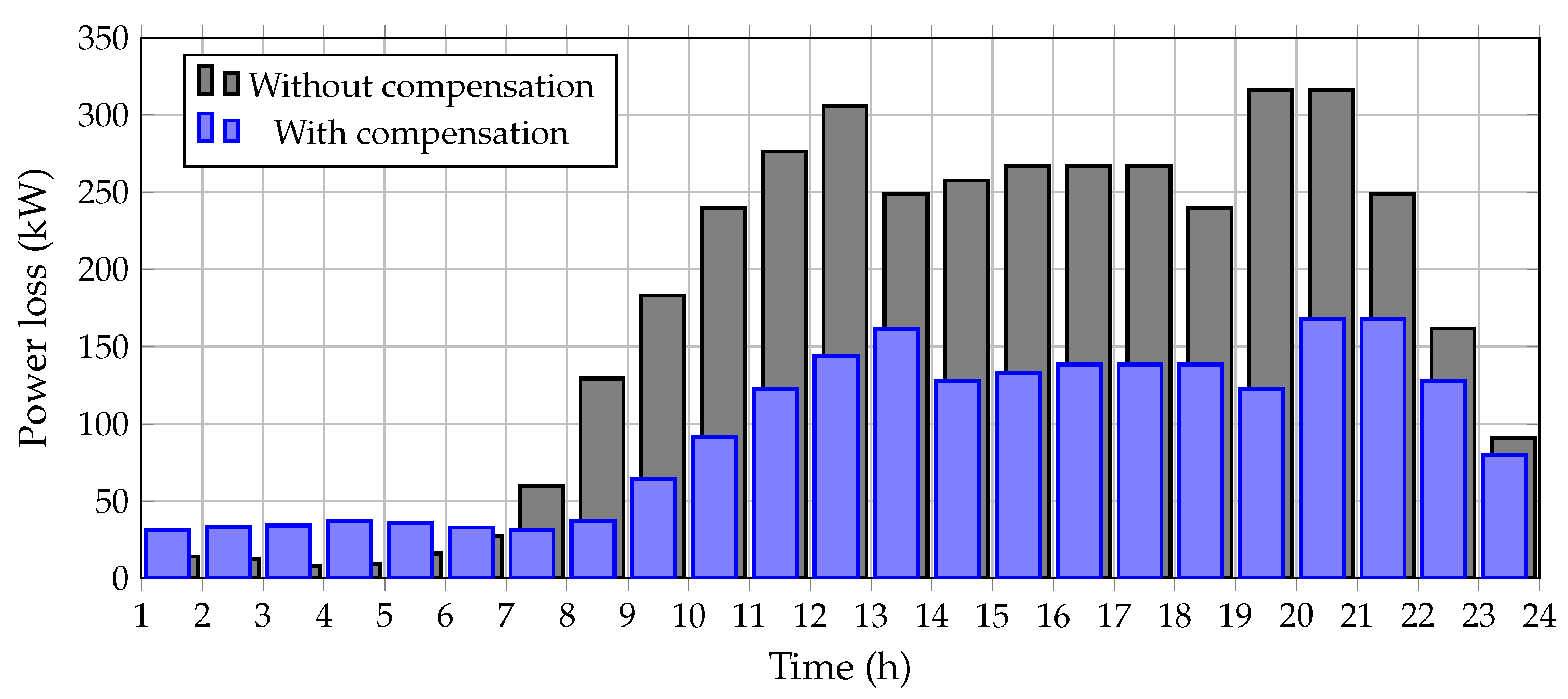
6.4.3. Complementary Analysis

It is important to mention that, in the studied simulation cases for the IEEE 85-bus grid, it was observed that: (i) the presence of dispersed generation helps with the expected costs of the annual grid power losses with a difference of USD/year 6610.92 compared to the case with zero PV injection; and (ii) the final position of the fixed-step capacitor banks and their optimal sizes are equal for both analyzed operation scenarios. This behavior can be attributed to a deficit in reactive power identified in these nodes, regardless of the active power variations on the grid.
On the other hand, Table 9 presents the comparative objective function value calculated with the approximated MIQC model (1)–(5) and the exact formula defined by Equation (11). Note that the fourth column is calculated as follows:
Error % = 100 % z approx z cost 2 z cost 2 ,
The numerical results shown by Table 9 allow stating that: (i) as expected, the mixed-integer convex model yields a better objective function value in comparison with the exact formula, given that the MIQC model (1)–(5) neglects the power losses caused by resistance in distribution lines and underestimates them using active and reactive power flows [33]; and (ii) the mean square errors calculated through Equation (13) show that the maximum error is present in the case of operation without fixed-step capacitor banks for the IEEE 69-bus system with a value of 2.961%, whereas the minimum error is evidenced in the case of operation with fixed-step capacitor banks for the IEEE 33-bus grid with a value of 0.692%. However, the most important finding in the fourth column of Table 9 is that all the estimation errors between the proposed MIQC formulation and the exact formula are lower than 3%, which confirms the effectiveness of this model at defining adequate locations for reactive power compensation via fixed-step capacitor banks.

7. Conclusions and Future Works

The problem concerning the optimal location and sizing of fixed-step capacitor banks in radial distribution networks was addressed in this research by implementing a two-stage optimization approach. The first optimization stage was entrusted with determining the set of nodes where the fixed-step capacitor banks were to be installed. To determine the optimal placement of these capacitors, a new MIQC model was proposed which allows for ensuring that the global optimum is reached due to the convexity of the solution space for each nodal capacitor placement combination. With the solution obtained from the MIQC model, the second optimization stage was fed, which corresponds to a recursive power flow solution to exhaustively evaluate all the capacitor size possibilities. Numerical results in distribution networks composed of 33, 69, and 85 nodes demonstrated the efficiency of the proposed two-stage optimization approach.
In the peak load scenario, the proposed two-stage optimization approach identified three better solutions for the IEEE 33-bus system in comparison with the GAMS software, as well as four better solutions in the case of the IEEE 69-bus grid. When the optimal solutions obtained for the proposed MIQC model and the recursive power flow solutions were compared with the the benchmark cases, the annual expected operating cost reductions were 33.04 and 34.29% for the IEEE 33- and IEEE 69-bus systems, respectively. In addition, the improvements with respect to the GAMS software for both test feeders were USD/year 111.996 and USD/year 31.664, respectively. These results validate the two-stage optimization approach as a new reference for studies regarding reactive power compensation in distribution networks using fixed-step capacitor banks.
In the case of the daily behavior of the demand consumption and the inclusion of PV generation, it was observed that: (i) the location and sizes of the fixed capacitors for the scenarios with and without penetration of the PV sources were the same, i.e., nodes 9, 34 and 67, with capacitor sizes of 600, 450, and 450 kvar, respectively, as these results confirmed that, for the IEEE 85-bus grid, there was a reactive deficit regardless of the active power generation available in the distribution grid; and (ii) the expected annual profits considering the daily demand behavior were USD/year 11,835.462 with respect to the simulation scenario without PV injection, and they were about USD/year 10,739.619 when PV sources were operated in the maximum power point tracking. These results showed that both simulations with a small investment in fixed-step capacitor banks reached reductions higher than 42% with respect to the benchmark cases.
Numerical comparisons between the exact formula in Equation (11) and the approximate objective function value defined in Equation (1) showed that, for all the simulation cases, the mean square error was lower than 3%, which confirmed the effectiveness of the proposed MIQC model at determining the better nodal location for the fixed-step capacitor banks in distribution networks with a radial configuration.
As future research, the following contributions could be made: (i) to extend the proposed optimization model to locate and size renewable generators and capacitor banks simultaneously in radial and meshed distribution networks; (ii) to apply the proposed optimization model to switched capacitor banks while including their loss model; and (iii) to develop an MIQC model to locate and size voltage regulators in distribution grids considering investment and operating costs.

Author Contributions

Formal analysis, O.D.M.; Investigation, O.D.M., E.R.-T. and D.A.G.-R.; Methodology, O.D.M.; Resources, O.D.M.; Writing—review & editing, O.D.M., E.R.-T. and D.A.G.-R. All authors have read and agreed to the published version of the manuscript.

Funding

This study was partially supported by the Center for Research and Scientific Development of Universidad Distrital Francisco José de Caldas, under grant 1643-12-2020 associated with the project Desarrollo de una metodología de optimización para la gestión óptima de recursos energéticos distribuidos en redes de distribución de energía eléctrica [Development of an optimization methodology for the optimal management of energy resources distributed across electrical energy distribution networks].

Institutional Review Board Statement

Not applicable.

Informed Consent Statement

Not applicable.

Data Availability Statement

No new data were created or analyzed in this study. Data sharing is not applicable to this paper.

Conflicts of Interest

The authors declare no conflict of interest.

References

  1. Picard, J.L.; Aguado, I.; Cobos, N.G.; Fuster-Roig, V.; Quijano-López, A. Electric Distribution System Planning Methodology Considering Distributed Energy Resources: A Contribution towards Real Smart Grid Deployment. Energies 2021, 14, 1924. [Google Scholar] [CrossRef]
  2. Kazmi, S.A.A.; Shahzad, M.K.; Khan, A.Z.; Shin, D.R. Smart Distribution Networks: A Review of Modern Distribution Concepts from a Planning Perspective. Energies 2017, 10, 501. [Google Scholar] [CrossRef]
  3. Malik, M.Z.; Kumar, M.; Soomro, A.M.; Baloch, M.H.; Farhan, M.; Gul, M.; Kaloi, G.S. Strategic planning of renewable distributed generation in radial distribution system using advanced MOPSO method. Energy Rep. 2020, 6, 2872–2886. [Google Scholar] [CrossRef]
  4. Montoya, O.D. Notes on the Dimension of the Solution Space in Typical Electrical Engineering Optimization Problems. Ingeniería 2022, 27, e19310. [Google Scholar] [CrossRef]
  5. Pareja, L.A.G.; Lezama, J.M.L.; Carmona, O.G. Optimal Placement of Capacitors, Voltage Regulators, and Distributed Generators in Electric Power Distribution Systems. Ingeniería 2020, 25, 334–354. [Google Scholar] [CrossRef]
  6. Zamani, A.; Sidhu, T.; Yazdani, A. A strategy for protection coordination in radial distribution networks with distributed generators. In Proceedings of the IEEE PES General Meeting, Minneapolis, MN, USA, 25–29 July 2010. [Google Scholar] [CrossRef]
  7. Castiblanco-Pérez, C.M.; Toro-Rodríguez, D.E.; Montoya, O.D.; Giral-Ramírez, D.A. Optimal Placement and Sizing of D-STATCOM in Radial and Meshed Distribution Networks Using a Discrete-Continuous Version of the Genetic Algorithm. Electronics 2021, 10, 1452. [Google Scholar] [CrossRef]
  8. Mahdavi, M.; Alhelou, H.H.; Hesamzadeh, M.R. An Efficient Stochastic Reconfiguration Model for Distribution Systems With Uncertain Loads. IEEE Access 2022, 10, 10640–10652. [Google Scholar] [CrossRef]
  9. Suesca, R.A.P.; León, A.I.S.; Rodríguez, C.L.T. Analysis for Selection of Battery-Based Storage Systems for Electrical Microgrids. Ingeniería 2020, 25, 284–304. (In Spanish) [Google Scholar] [CrossRef]
  10. The, T.T.; Ngoc, D.V.; Anh, N.T. Distribution Network Reconfiguration for Power Loss Reduction and Voltage Profile Improvement Using Chaotic Stochastic Fractal Search Algorithm. Complexity 2020, 2020, 2353901. [Google Scholar] [CrossRef]
  11. Zhan, J.; Liu, W.; Chung, C.Y.; Yang, J. Switch Opening and Exchange Method for Stochastic Distribution Network Reconfiguration. IEEE Trans. Smart Grid 2020, 11, 2995–3007. [Google Scholar] [CrossRef]
  12. Görbe, P.; Magyar, A.; Hangos, K.M. Reduction of power losses with smart grids fueled with renewable sources and applying EV batteries. J. Clean. Prod. 2012, 34, 125–137. [Google Scholar] [CrossRef]
  13. Montoya, O.D.; Grisales-Noreña, L.F.; Alvarado-Barrios, L.; Arias-Londoño, A.; Álvarez-Arroyo, C. Efficient Reduction in the Annual Investment Costs in AC Distribution Networks via Optimal Integration of Solar PV Sources Using the Newton Metaheuristic Algorithm. Appl. Sci. 2021, 11, 11525. [Google Scholar] [CrossRef]
  14. Chedid, R.; Sawwas, A. Optimal placement and sizing of photovoltaics and battery storage in distribution networks. Energy Storage 2019, 1, e46. [Google Scholar] [CrossRef] [Green Version]
  15. Rastogi, M.; Bhat, A.H. Reactive power compensation using static synchronous compensator (STATCOM) with conventional control connected with 33kV grid. In Proceedings of the 2015 2nd International Conference on Recent Advances in Engineering & Computational Sciences (RAECS), Chandigarh, India, 21–22 December 2015. [Google Scholar] [CrossRef]
  16. Gallego, R.; Monticelli, A.; Romero, R. Optimal capacitor placement in radial distribution networks. IEEE Trans. Power Syst. 2001, 16, 630–637. [Google Scholar] [CrossRef]
  17. Abdelaziz, A.; Ali, E.; Elazim, S.A. Optimal sizing and locations of capacitors in radial distribution systems via flower pollination optimization algorithm and power loss index. Eng. Sci. Technol. Int. J. 2016, 19, 610–618. [Google Scholar] [CrossRef] [Green Version]
  18. Riaño, F.E.; Cruz, J.F.; Montoya, O.D.; Chamorro, H.R.; Alvarado-Barrios, L. Reduction of Losses and Operating Costs in Distribution Networks Using a Genetic Algorithm and Mathematical Optimization. Electronics 2021, 10, 419. [Google Scholar] [CrossRef]
  19. Tamilselvan, V.; Jayabarathi, T.; Raghunathan, T.; Yang, X.S. Optimal capacitor placement in radial distribution systems using flower pollination algorithm. Alex. Eng. J. 2018, 57, 2775–2786. [Google Scholar] [CrossRef]
  20. Gil-González, W.; Montoya, O.D.; Rajagopalan, A.; Grisales-Noreña, L.F.; Hernández, J.C. Optimal Selection and Location of Fixed-Step Capacitor Banks in Distribution Networks Using a Discrete Version of the Vortex Search Algorithm. Energies 2020, 13, 4914. [Google Scholar] [CrossRef]
  21. Montoya, O.D.; Gil-González, W.; Garcés, A. On the Conic Convex Approximation to Locate and Size Fixed-Step Capacitor Banks in Distribution Networks. Computation 2022, 10, 32. [Google Scholar] [CrossRef]
  22. Soma, G.G. Optimal Sizing and Placement of Capacitor Banks in Distribution Networks Using a Genetic Algorithm. Electricity 2021, 2, 187–204. [Google Scholar] [CrossRef]
  23. Tabatabaei, S.; Vahidi, B. Bacterial foraging solution based fuzzy logic decision for optimal capacitor allocation in radial distribution system. Electr. Power Syst. Res. 2011, 81, 1045–1050. [Google Scholar] [CrossRef]
  24. Kavousi-Fard, A.; Samet, H. Multi-objective Performance Management of the Capacitor Allocation Problem in Distributed System Based on Adaptive Modified Honey Bee Mating Optimization Evolutionary Algorithm. Electr. Power Components Syst. 2013, 41, 1223–1247. [Google Scholar] [CrossRef]
  25. El-Fergany, A.A.; Abdelaziz, A.Y. Cuckoo Search-based Algorithm for Optimal Shunt Capacitors Allocations in Distribution Networks. Electr. Power Compon. Syst. 2013, 41, 1567–1581. [Google Scholar] [CrossRef]
  26. Devabalaji, K.; Yuvaraj, T.; Ravi, K. An efficient method for solving the optimal sitting and sizing problem of capacitor banks based on cuckoo search algorithm. Ain Shams Eng. J. 2018, 9, 589–597. [Google Scholar] [CrossRef] [Green Version]
  27. El-Fergany, A.A.; Abdelaziz, A.Y. Artificial Bee Colony Algorithm to Allocate Fixed and Switched Static Shunt Capacitors in Radial Distribution Networks. Electr. Power Compon. Syst. 2014, 42, 427–438. [Google Scholar] [CrossRef]
  28. Sedighizadeh, M.; Bakhtiary, R. Optimal multi-objective reconfiguration and capacitor placement of distribution systems with the Hybrid Big Bang–Big Crunch algorithm in the fuzzy framework. Ain Shams Eng. J. 2016, 7, 113–129. [Google Scholar] [CrossRef] [Green Version]
  29. Sambaiah, K.S.; Jayabarathi, T. Optimal Allocation of Renewable Distributed Generation and Capacitor Banks in Distribution Systems using Salp Swarm Algorithm. Int. J. Renew. Energy Res. 2019, 9, 96–107. [Google Scholar] [CrossRef]
  30. Sadeghian, O.; Oshnoei, A.; Kheradmandi, M.; Mohammadi-Ivatloo, B. Optimal placement of multi-period-based switched capacitor in radial distribution systems. Comput. Electr. Eng. 2020, 82, 106549. [Google Scholar] [CrossRef]
  31. Tahir, M.J.; Rasheed, M.B.; Rahmat, M.K. Optimal Placement of Capacitors in Radial Distribution Grids via Enhanced Modified Particle Swarm Optimization. Energies 2022, 15, 2452. [Google Scholar] [CrossRef]
  32. Lei, T.; Riaz, S.; Raziq, H.; Batool, M.; Pan, F.; Wang, J. A Comparison of Metaheuristic Techniques for Solving Optimal Sitting and Sizing Problems of Capacitor Banks to Reduce the Power Loss in Radial Distribution System. Complexity 2022, 2022, 4547212. [Google Scholar] [CrossRef]
  33. Taylor, J.A.; Hover, F.S. Convex Models of Distribution System Reconfiguration. IEEE Trans. Power Syst. 2012, 27, 1407–1413. [Google Scholar] [CrossRef]
  34. Marini, A.; Mortazavi, S.; Piegari, L.; Ghazizadeh, M.S. An efficient graph-based power flow algorithm for electrical distribution systems with a comprehensive modeling of distributed generations. Electr. Power Syst. Res. 2019, 170, 229–243. [Google Scholar] [CrossRef]
  35. Montoya, O.D.; Rivas-Trujillo, E.; Hernández, J.C. A Two-Stage Approach to Locate and Size PV Sources in Distribution Networks for Annual Grid Operative Costs Minimization. Electronics 2022, 11, 961. [Google Scholar] [CrossRef]
  36. Farivar, M.; Low, S.H. Branch Flow Model: Relaxations and Convexification—Part I. IEEE Trans. Power Syst. 2013, 28, 2554–2564. [Google Scholar] [CrossRef]
  37. Montoya, O.D.; Moya, F.D.; Rajagopalan, A. Annual Operating Costs Minimization in Electrical Distribution Networks via the Optimal Selection and Location of Fixed-Step Capacitor Banks Using a Hybrid Mathematical Formulation. Mathematics 2022, 10, 1600. [Google Scholar] [CrossRef]
  38. Montoya, O.D.; Gil-González, W. On the numerical analysis based on successive approximations for power flow problems in AC distribution systems. Electr. Power Syst. Res. 2020, 187, 106454. [Google Scholar] [CrossRef]
  39. Herrera-Briñez, M.C.; Montoya, O.D.; Alvarado-Barrios, L.; Chamorro, H.R. The Equivalence between Successive Approximations and Matricial Load Flow Formulations. Appl. Sci. 2021, 11, 2905. [Google Scholar] [CrossRef]
  40. Shen, T.; Li, Y.; Xiang, J. A Graph-Based Power Flow Method for Balanced Distribution Systems. Energies 2018, 11, 511. [Google Scholar] [CrossRef] [Green Version]
  41. Zhang, D.; Fu, Z.; Zhang, L. An improved TS algorithm for loss-minimum reconfiguration in large-scale distribution systems. Electr. Power Syst. Res. 2007, 77, 685–694. [Google Scholar] [CrossRef]
  42. Soroudi, A. Power System Optimization Modeling in GAMS; Springer International Publishing: Berlin/Heidelberg, Germany, 2017. [Google Scholar] [CrossRef]
  43. Shuaib, Y.M.; Kalavathi, M.S.; Rajan, C.C.A. Optimal capacitor placement in radial distribution system using Gravitational Search Algorithm. Int. J. Electr. Power Energy Syst. 2015, 64, 384–397. [Google Scholar] [CrossRef]
  44. Abul’Wafa, A.R. Optimal capacitor placement for enhancing voltage stability in distribution systems using analytical algorithm and Fuzzy-Real Coded GA. Int. J. Electr. Power Energy Syst. 2014, 55, 246–252. [Google Scholar] [CrossRef]
  45. Sultana, S.; Roy, P.K. Optimal capacitor placement in radial distribution systems using teaching learning based optimization. Int. J. Electr. Power Energy Syst. 2014, 54, 387–398. [Google Scholar] [CrossRef]
Figure 1. Test feeder grid configuration: (a) IEEE 33- and (b) IEEE 69-node system.
Computers 11 00105 g001
Figure 2. Electrical configuration of the IEEE 85-bus grid.
Computers 11 00105 g002
Figure 3. Expected behavior of the demand and PV generation for a typically sunny day.
Computers 11 00105 g003
Figure 4. Daily behavior of power losses without considering PV injection.
Computers 11 00105 g004
Figure 5. Daily behavior of power losses considering PV injection.
Computers 11 00105 g005
Table 1. Some recent literature approaches to locating and sizing capacitor banks in distribution networks.
Solution MethodologyObjective FunctionYearRef.
Bacterial foraging algorithm combined with fuzzy logicExpected annual energy loss costs2011 [23]
Modified honey bee mating optimization evolutionary algorithmMinimizing power losses and improving the voltage profile as well as annual investment and operating costs2013 [24]
Cuckoo search-based algorithmAnnual investment and operating costs2013, 2018 [25,26]
Artificial bee colony optimization algorithmAnnual investment and operating costs2014 [27]
Big bang/big crunch algorithm and fuzzy logicMinimizing power losses, improving the voltage profile, and reducing the grid voltage imbalance2016 [28]
Flower pollination algorithmAnnual investment and operating costs2016, 2018 [17,19]
Salp swarm optimizationPower loss minimization and voltage profile improvement2019 [29]
Recursive power flow evaluations and loss sensitive factorsPower loss minimization and voltage profile improvement2020 [30]
Chu and Beasley and specialized genetic algorithmsAnnual investment and operating costs2020, 2021 [5,18]
Particle swarm optimizationAnnual investment and operating costs2022 [31]
Bat optimization algorithmMinimization of power loss2022 [32]
Modified particle swarm optimization methodAnnual investment and operating costs2022 [31]
Table 2. IEEE 33-bus system parameters.
Node iNode jRij (Ω)Xij (Ω)Pj (kW)Qj (kvar)Node iNode jRij (Ω)Xij (Ω)Pj (kW)Qj (kvar)
120.09220.04771006017180.73200.57409040
230.49300.251190402190.16400.15659040
340.36600.18641208019201.50421.35549040
450.38110.1941603020210.40950.47849040
560.81900.7070602021220.70890.93739040
670.18720.61882001003230.45120.30839050
781.71141.235120010023240.89800.7091420200
891.03000.7400602024250.89600.7011420200
9101.04000.740060206260.20300.10346025
10110.19660.0650453026270.28420.14476025
11120.37440.1238603527281.05900.93376020
12131.46801.1550603528290.80420.700612070
13140.54160.71291208029300.50750.2585200600
14150.59100.5260601030310.97440.963015070
15160.74630.5450602031320.31050.3619210100
16171.28601.7210602032330.34100.53026040
Table 3. Parametric information of the IEEE 69-bus system.
Node iNode jRij (Ω)Xij (Ω)Pj (kW)Qj (kvar)Node iNode jRij (Ω)Xij (Ω)Pj (kW)Qj (kvar)
120.00050.0012003360.00440.01082618.55
230.00050.00120036370.06400.15652618.55
340.00150.00360037380.10530.123000
450.02510.02940038390.03040.03552417
560.36600.18642.62.239400.00180.00212417
670.38100.194140.43040410.72830.85091.21
780.09220.0470755441420.31000.362300
890.04930.0251302242430.04100.047564.3
9100.81900.2707281943440.00920.011600
10110.18720.061914510444450.10890.137339.2226.3
11120.71140.235114510445460.00090.001239.2226.3
12131.03000.3400854470.00340.008400
13141.04400.345085.547480.08510.20837956.4
14151.05800.34960048490.28980.7091384.7274.5
15160.19660.065045.53049500.08220.2011384.7274.5
16170.37440.123860358510.09280.047340.528.3
17180.00470.0016603551520.33190.11143.62.7
18190.32760.1083009530.17400.08864.353.5
19200.21060.069010.653540.20300.103426.419
20210.34160.11291148154550.28420.14472417.2
21220.01400.004653.555560.28130.143300
22230.15910.05260056571.59000.533700
23240.34600.1145282057580.78370.263000
24250.74880.24750058590.30420.100610072
25260.30890.1021141059600.38610.117200
26270.17320.0572141060610.50750.25851244888
3280.00440.01082618.661620.09740.04963223
28290.06400.15652618.662630.14500.073800
29300.39780.13150063640.71050.3619227162
30310.07020.02320064651.04100.53025942
31320.35100.11600011660.20120.06111813
32330.83900.2816141066670.00470.00141813
33341.70800.564619.51412680.73940.24442820
34351.47400.48736468690.00470.00162820
Table 4. Parametric information of the IEEE 85-bus system.
Node iNode jRij (Ω)Xij (Ω)Pj (kW)Qj (kvar)Node iNode jRij (Ω)Xij (Ω)Pj (kW)Qj (kvar)
120.1080.0750034441.0020.41635.2835.99
230.1630.1120044450.9110.37835.2835.99
340.2170.1495657.1345460.9110.37835.2835.99
450.1080.0740046470.5460.2261414.28
560.4350.29835.2835.9935480.6370.26400
670.2720.1860048490.1820.07500
781.1970.82035.2835.9949500.3640.15136.2837.01
890.1080.0740050510.4550.1895657.13
9100.5980.4100048521.3660.56700
10110.5440.3735657.1352530.4550.18935.2835.99
11120.5440.3730053540.5460.2265657.13
12130.5980.4100052550.5460.2265657.13
13140.2720.18635.2835.9949560.5460.2261414.28
14150.3260.22335.2835.999570.2730.1135657.13
2160.7280.30235.2835.9957580.8190.34000
3170.4550.189112114.2658590.1820.0755657.13
5180.8200.3405657.1358600.5460.2265657.13
18190.6370.2645657.1360610.7280.3025657.13
19200.4550.18935.2835.9961621.0020.4155657.13
20210.8190.34035.2835.9960630.1820.0751414.28
21221.5480.64235.2835.9963640.7280.30200
19230.1820.0755657.1364650.1820.07500
7240.9100.37835.2835.9965660.1820.0755657.13
8250.4550.18935.2835.9964670.4550.18900
25260.3640.1515657.1367680.9100.37800
26270.5460.2260068691.0920.4535657.13
27280.2730.1135657.1369700.4550.18900
28290.5460.2260070710.5460.22635.2835.99
29300.5460.22635.2835.9967720.1820.0755657.13
30310.2730.11335.2835.9968731.1840.49100
31320.1820.0750073740.2730.1135657.13
32330.1820.0751414.2873751.0020.41635.2835.99
33340.8190.3400070760.5460.2265657.13
34350.6370.2640065770.0910.0371414.28
35360.1820.07535.2835.9910780.6370.2645657.13
26370.3640.1515657.1367790.5460.22635.2835.99
27381.0020.4165657.1312800.7280.3025657.13
29390.5460.2265657.1380810.3640.15100
32400.4550.18935.2835.9981820.0910.0375657.13
40411.0020.4160081831.0920.45335.2835.99
41420.2730.11335.2835.9983841.0020.4161414.28
41430.4550.18935.2835.9913850.8190.34035.2835.99
Table 5. Costs of the capacitors according to their capacity.
OptionQc (kvar)Cost (USD/kvar-year)OptionQc (kvar)Cost (USD/kvar-year)
11500.500812000.170
23000.350913500.207
34500.2531015000.201
46000.2201116500.193
57500.2761218000.870
69000.1831319500.211
710500.2281421000.176
Table 6. Comparative results between the two-stage approach and multiple literature reports.
MethodSize (Node) (Mvar)Losses (kW)
IEEE 33-bus grid
Benc. Case-210.987
AM{0.45(9), 0.80(29), 0.90(30)}171.780
TSM{0.85(7), 0.025(29), 0.90(30)}144.040
FRCGA{0.475(6), 0.175(8), 0.35(9), 0.025(28), 0.30(29), 0.40(30)}141.240
FPA{0.45(13), 0.45(24), 0.90(30)}139.075
GAMS{0.30(14), 0.45(24), 1.05(30)}139.292
MIQC{0.45(13), 0.45(24), 1.05(30)}138.473
IEEE 69-bus grid
Benc. Case-225.072
AM{0.90(11), 1.05(29), 0.45(60)}163.280
TSM{0.225(19), 0.90(62), 0.225(63)}148.910
TBLO{0.60(12), 1.05(61), 0.15(64)}146.350
FPA{0.45(11), 0.15(22), 1.35(61)}145.860
GAMS{0.45(11), 0.15(27), 1.20(61)}145.738
MIQC{0.45(11), 0.15(21), 1.20(61)}145.550
Table 7. Comparative results between the GAMS and the proposed MIQC proposal, IEEE 33-bus grid.
MethodSize (Node) (Mvar)Losses (kW)C. Caps. USDC. Total USD
GAMS{0.30(14), 0.45(24), 1.05(30)}139.292458.2523,859.313
MIQC (sol. 1){0.45(13), 0.45(24), 1.05(30)}138.473467.1023,747.317
MIQC (sol. 2){0.45(13), 0.60(24), 0.90(30)}138.917410.5523,748.531
MIQC (sol. 3){0.45(13), 0.45(24), 0.90(30)}139.075392.4023,757.083
Table 8. Comparative results between GAMS and the MIQC proposal for the IEEE 69-bus test feeder.
MethodSize (Node) (Mvar)Losses (kW)C. Caps. USDC. Total USD
GAMS{0.45(11), 0.15(27), 1.20(61)}145.738392.8524,876.910
MIQC (sol. 1){0.45(11), 0.15(21), 1.20(61)}145.550392.8524,845.246
MIQC (sol. 2){0.30(11), 0.30(21), 1.20(61)}145.492414.0024,856.573
MIQC (sol. 3){0.60(11), 0.15(21), 1.20(61)}145.614411.0024,874.173
MIQC (sol. 4){0.45(11), 0.30(21), 1.20(61)}145.556422.8524,876.229
Table 9. Comparative results between the approximated MIQC model and the exact objective function calculation.
Without fixed-step capacitor bank
System z approx z cos t Error (%)
IEEE 33-bus system30,605.56835,445.9091.865
IEEE 69-bus system32,186.28937,812.0562.214
IEEE 85-bus system (without PV)23,119.56027,924.7932.961
IEEE 85-bus system (with PV)18,309.42821,313.8721.987
With fixed-step capacitor bank
System z approx z cos t Error (%)
IEEE 33-bus system21,771.32023,747.3180.692
IEEE 69-bus system22,159.46724,845.2471.169
IEEE 85-bus system (without PV)14,430.46616,089.3311.063
IEEE 85-bus system (with PV)9620.33510,574.2530.814
Publisher’s Note: MDPI stays neutral with regard to jurisdictional claims in published maps and institutional affiliations.

