
Assessment of SQL and NoSQL Systems to Store and Mine COVID-19 Data


Abstract
:
1. Introduction
2. Related Work
2.1. SQL versus NoSQL Databases
2.2. Data Mining on COVID-19 Data
3. Data Mining
3.1. Algorithms
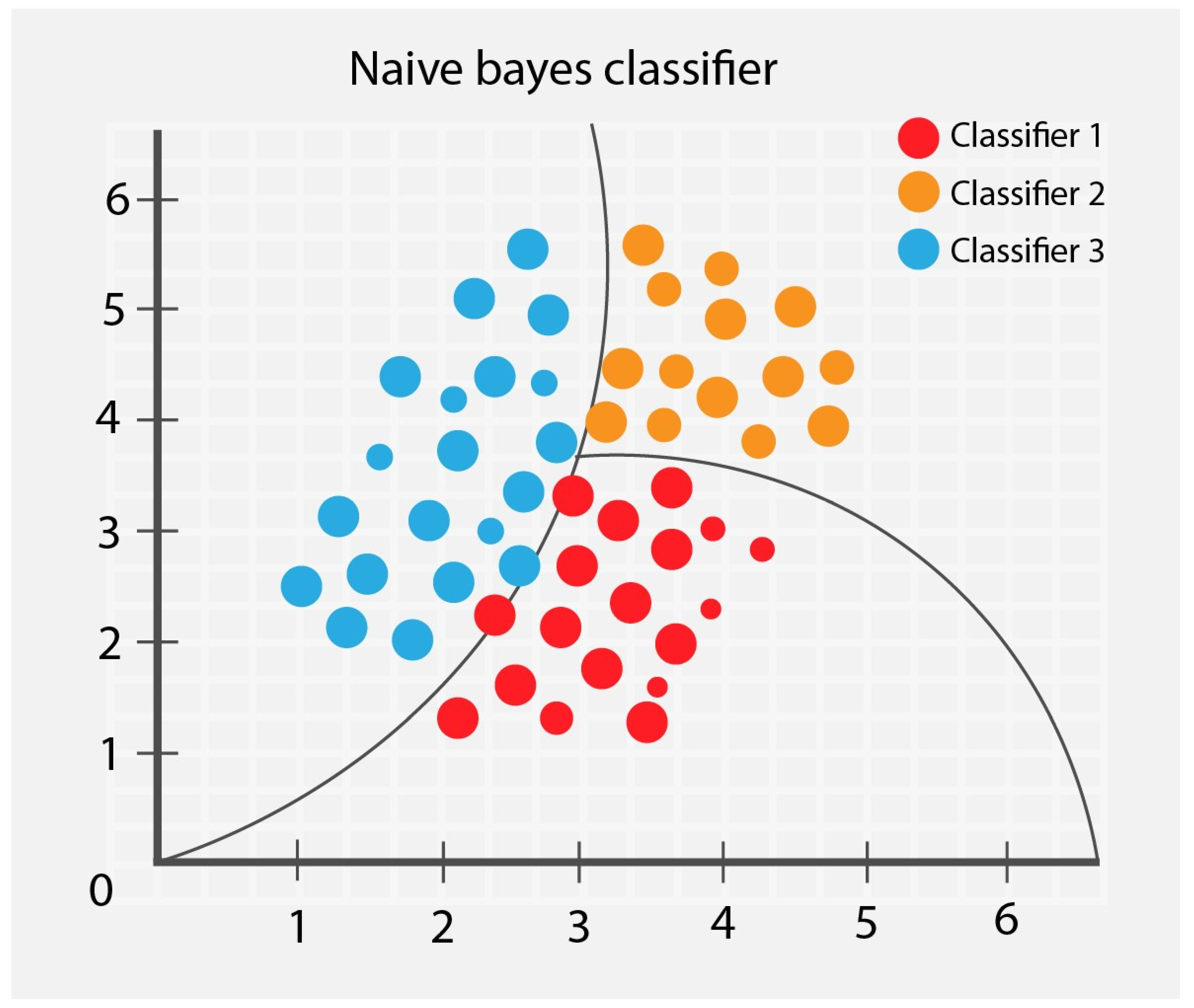
3.1.1. Naïve Bayes
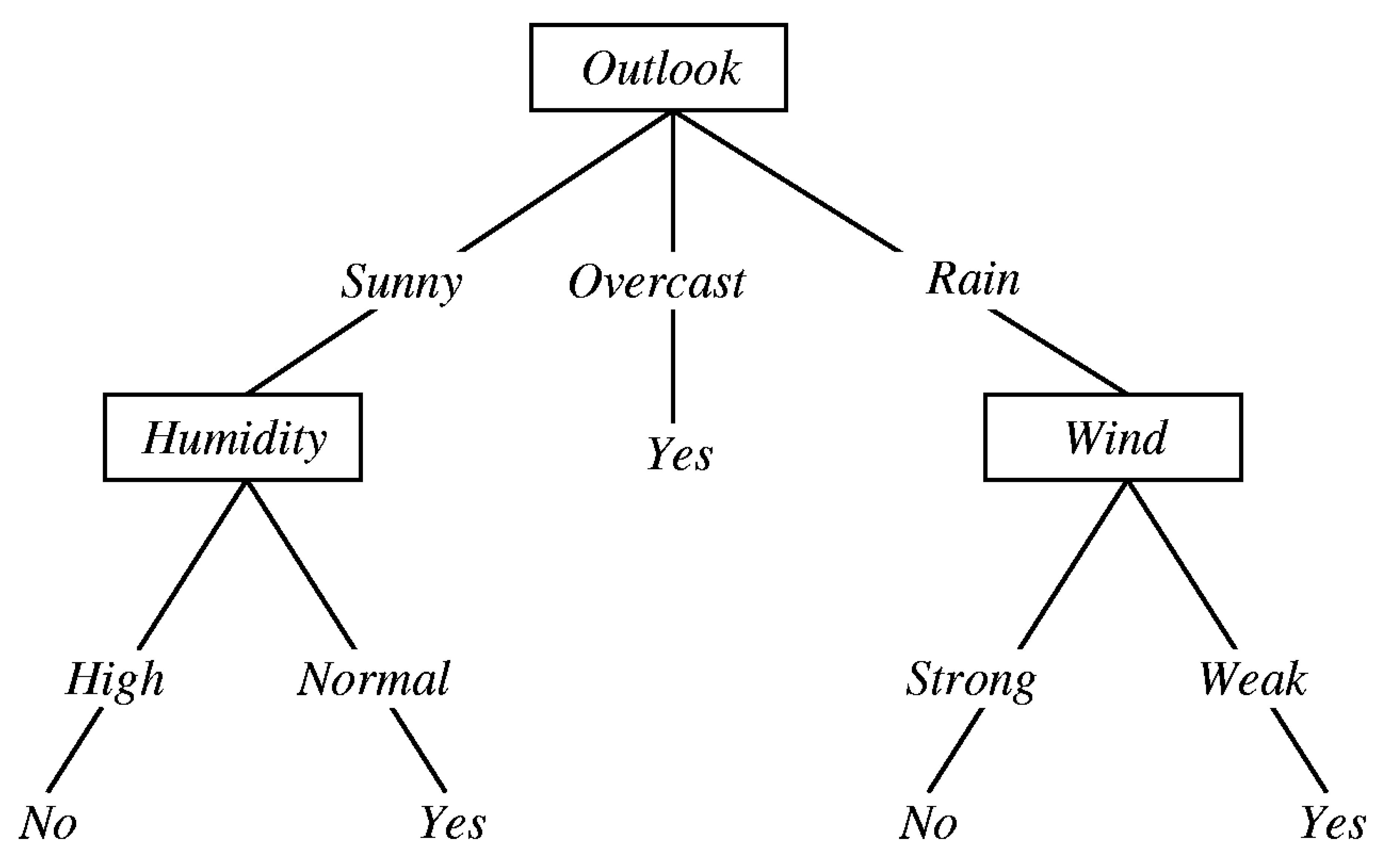
3.1.2. Decision Tree
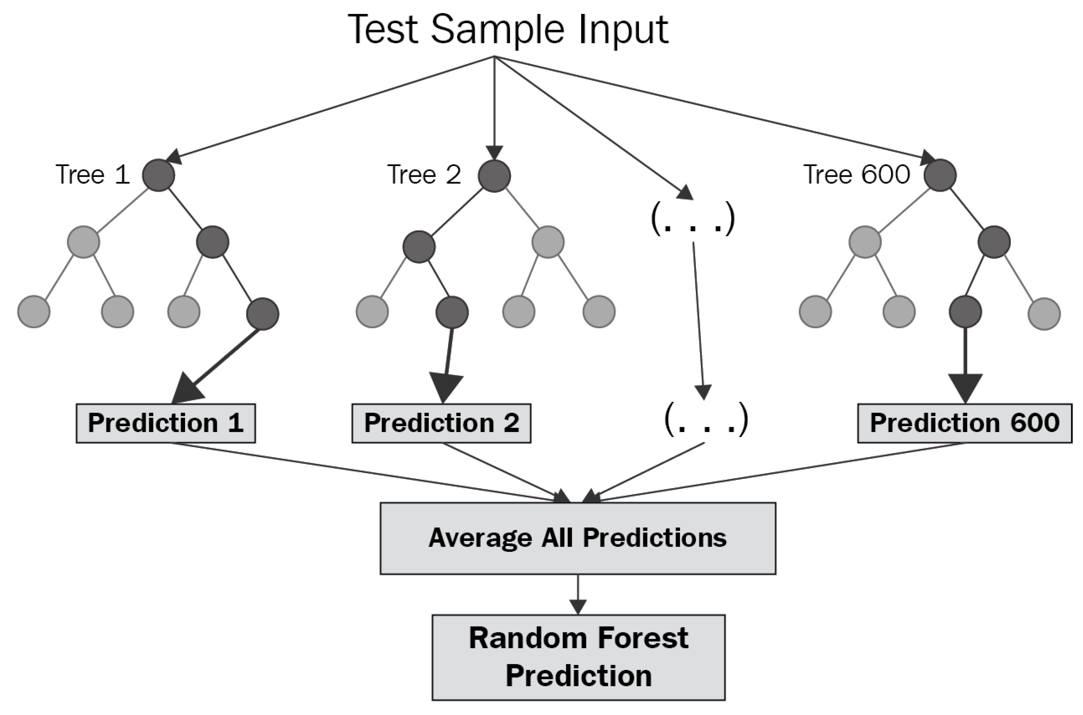
3.1.3. Random Forest
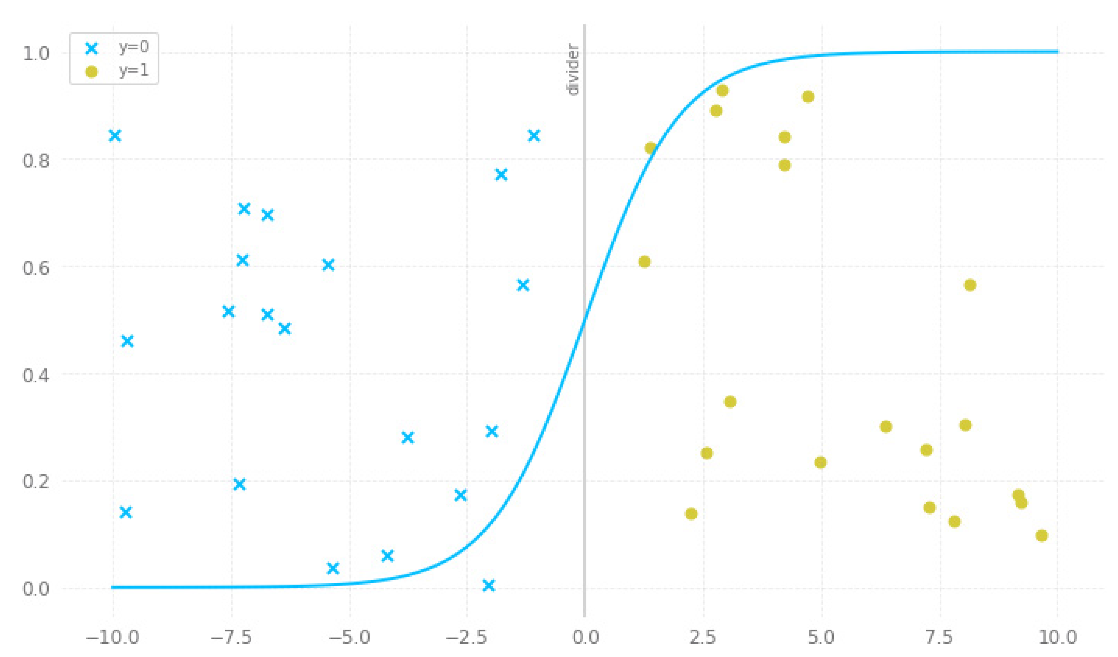
3.1.4. Logistic Regression
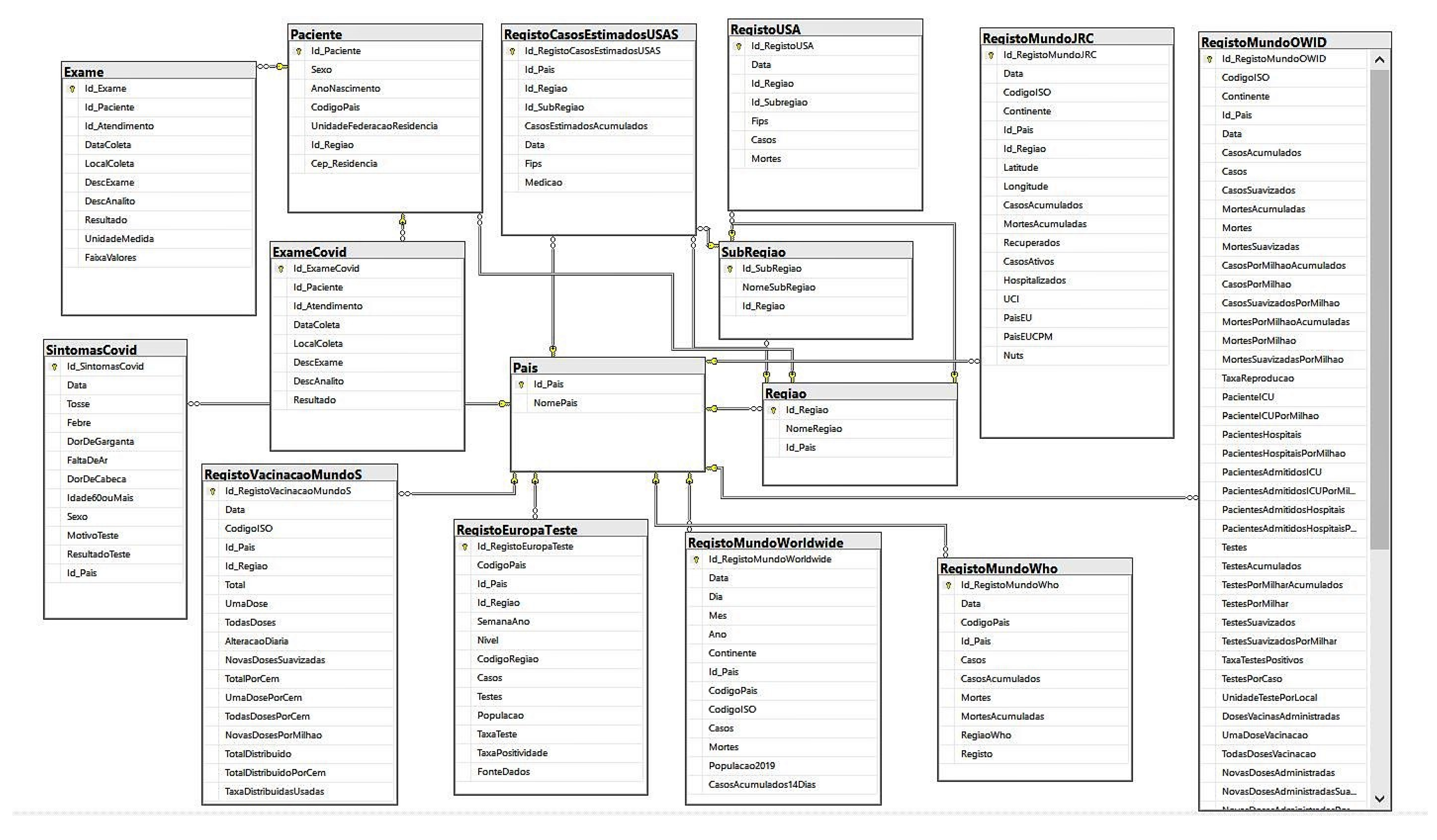
4. Data Modeling
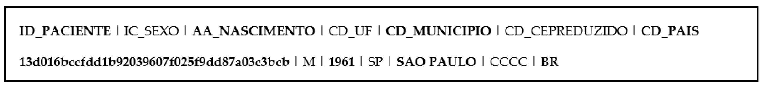
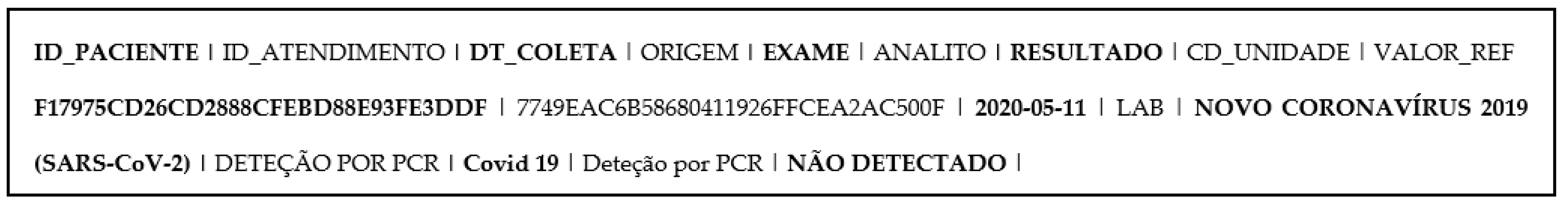
Data Extraction
5. Experimental Evaluation
5.1. Data Mining Experiments—Classification Tests
- I—Target: TestResult; 3 Possibilities: Negative (0), Positive (1), Inconclusive (2);
- II—Target: Cough; 2 Possibilities: Positive (1), Negative (0);
- III—Target: Fever; 2 Possibilities: Positive (1), Negative (0);
- IV—Target: SoreThroat; 2 Possibilities: Positive (1), Negative (0);
- V—Target: ShortnessOfBreath; 2 Possibilities: Positive (1), Negative (0);
- VI—Target: Headache; 2 Possibilities: Positive (1), Negative (0).
- VII—Target: CoughTestResult; 6 Possibilities: Positive for cough and Negative for test result (10), Positive for both (11), Positive for cough and Inconclusive for test result (12), Negative for both (00), Negative for cough and Positive for test result (01), Negative for cough and Inconclusive for test result (02);
- VIII—Target: FeverTestResult; 6 Possibilities: Positive for fever and Negative for test result (10), Positive for both (11), Positive for fever and Inconclusive for test result (12), Negative for both (00), Negative for fever and Positive for test result (01), Negative for fever and Inconclusive for test result (02);
- IX—Target: SoreThroatTestResult; 6 Possibilities: Positive for sore throat and Negative for test result (10), Positive for both (11), Positive for sore throat and Inconclusive for test result (12), Negative for both (00), Negative for sore throat and Positive for test result (01), Negative for sore throat and Inconclusive for test result (02);
- X—Target: ShortnessOfBreathTestResult; 6 Possibilities: Positive for shortness of breath and Negative for test result (10), Positive for both (11), Positive for shortness of breath and Inconclusive for test result (12), Negative for both (00), Negative for shortness of breath and Positive for test result (01), Negative for shortness of breath and Inconclusive for test result (02);
- XI—Target: HeadacheTestResult; 6 Possibilities: Positive for headache and Negative for test result (10), Positive for both (11), Positive for headache and Inconclusive for test result (12), Negative for both (00), Negative for headache and Positive for test result (01), Negative for headache and Inconclusive for test result (02);
- XII—Target: CoughShortnessOfBreathTestResult; 12 Possibilities: Negative for all (000), Negative for cough and shortness of breath and Positive for test result (001), Negative for cough and test result and Positive for shortness of breath (010), Negative for cough and Positive for shortness of breath and test result (011), Positive for cough and Negative for shortness of breath and test result (100), Positive for cough and test result and Negative for shortness of breath (101), Positive for cough and shortness of breath and Negative for test result (110), Positive for all (111), Negative for cough and shortness of breath and Inconclusive for test result (002), Positive for cough, Negative for shortness of breath and Inconclusive for test result (102), Negative for cough, Positive for shortness of breath and Inconclusive for test result (012), Positive for cough and shortness of breath and Inconclusive for test result (112);
- XIII—Target: FeverHeadacheTestResult; 12 Possibilities: (000), (001), (010), (011), (100), (101), (110), (111), (002), (102), (012), (112);
- XIV—Target: SoreThroatShortnessOfBreathTestResult; 12 Possibilities: (000), (001), (010), (011), (100), (101), (110), (111), (002), (102), (012), (112).
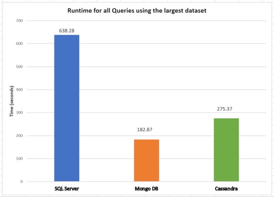
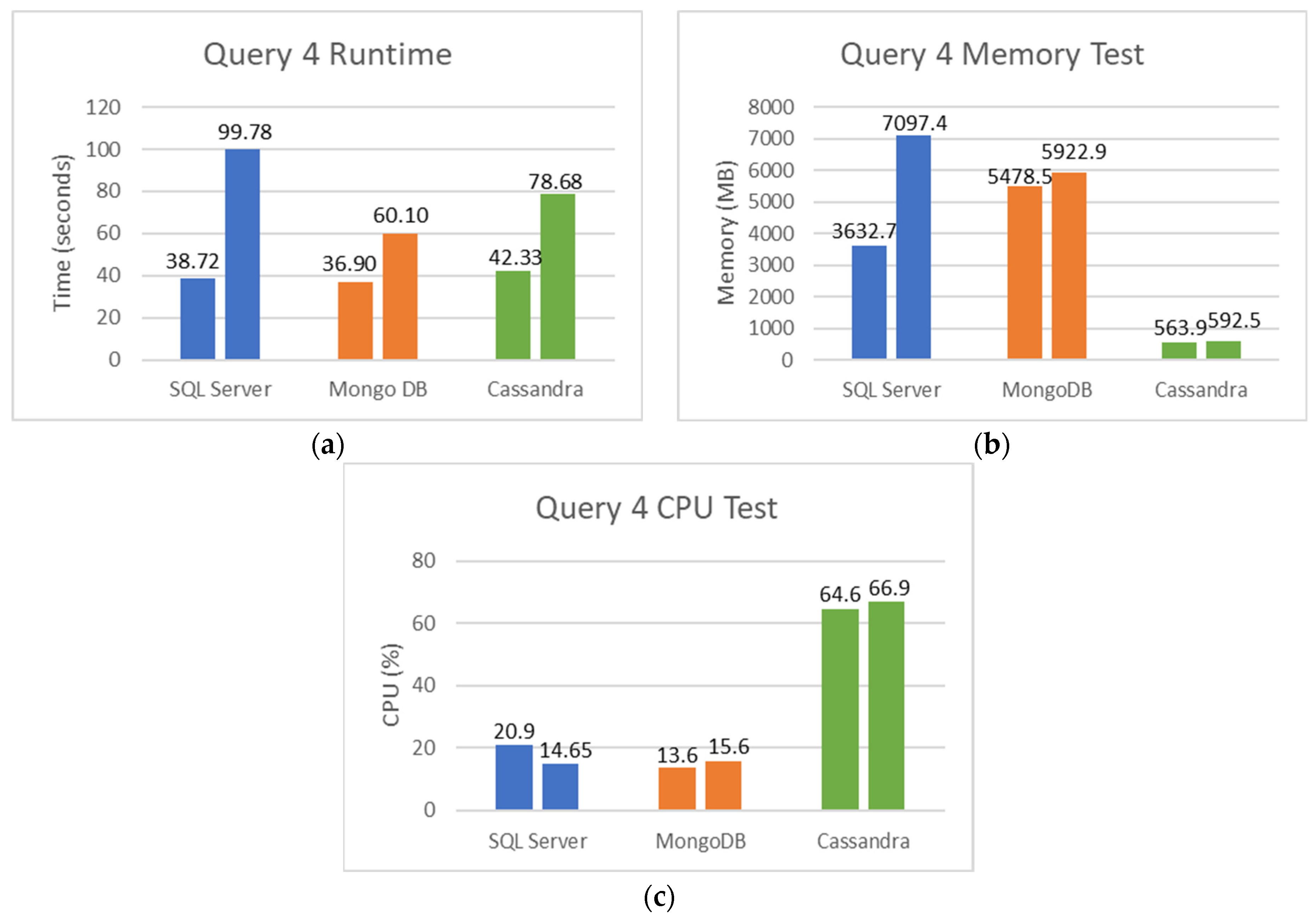
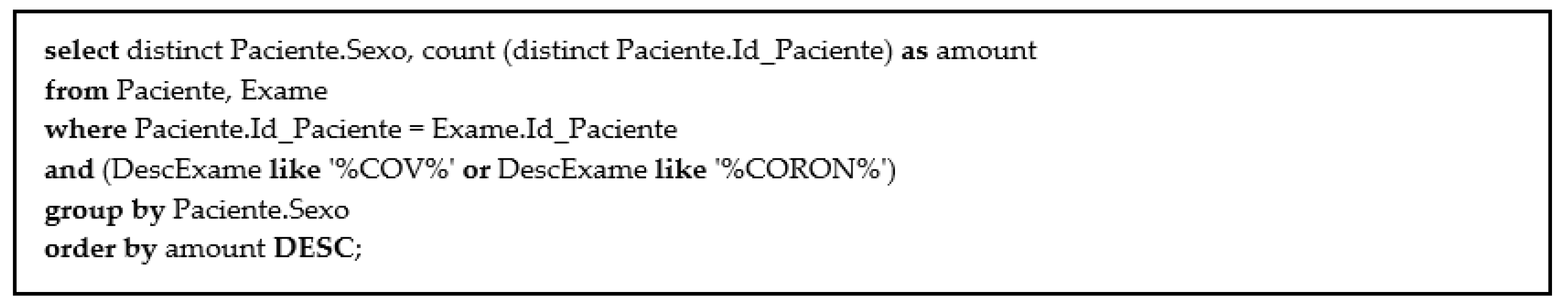
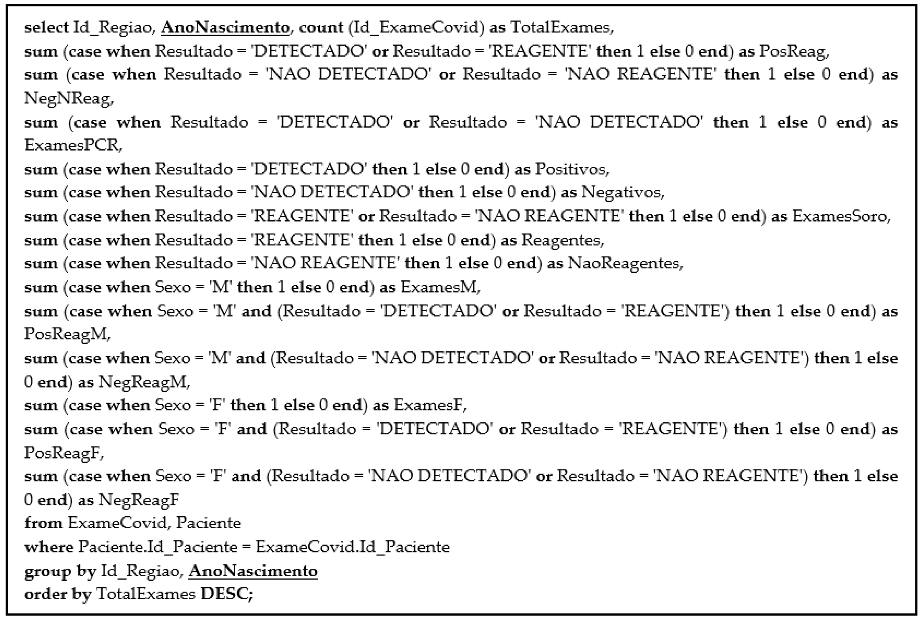
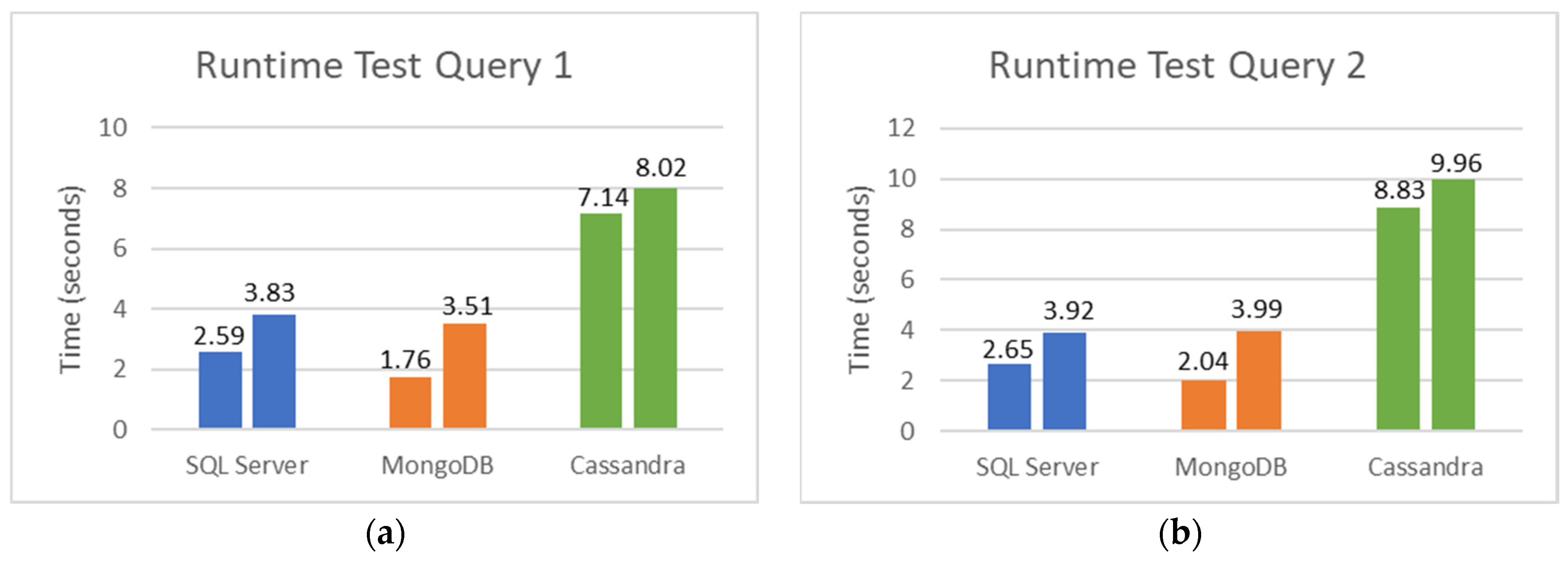
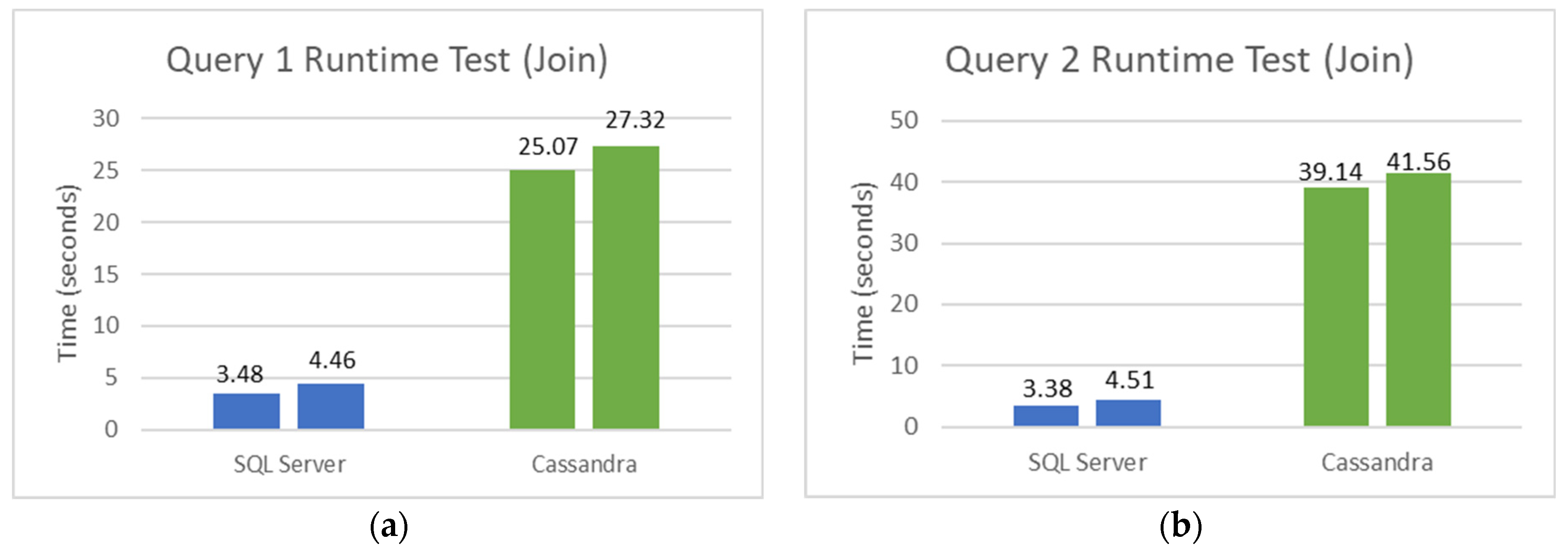
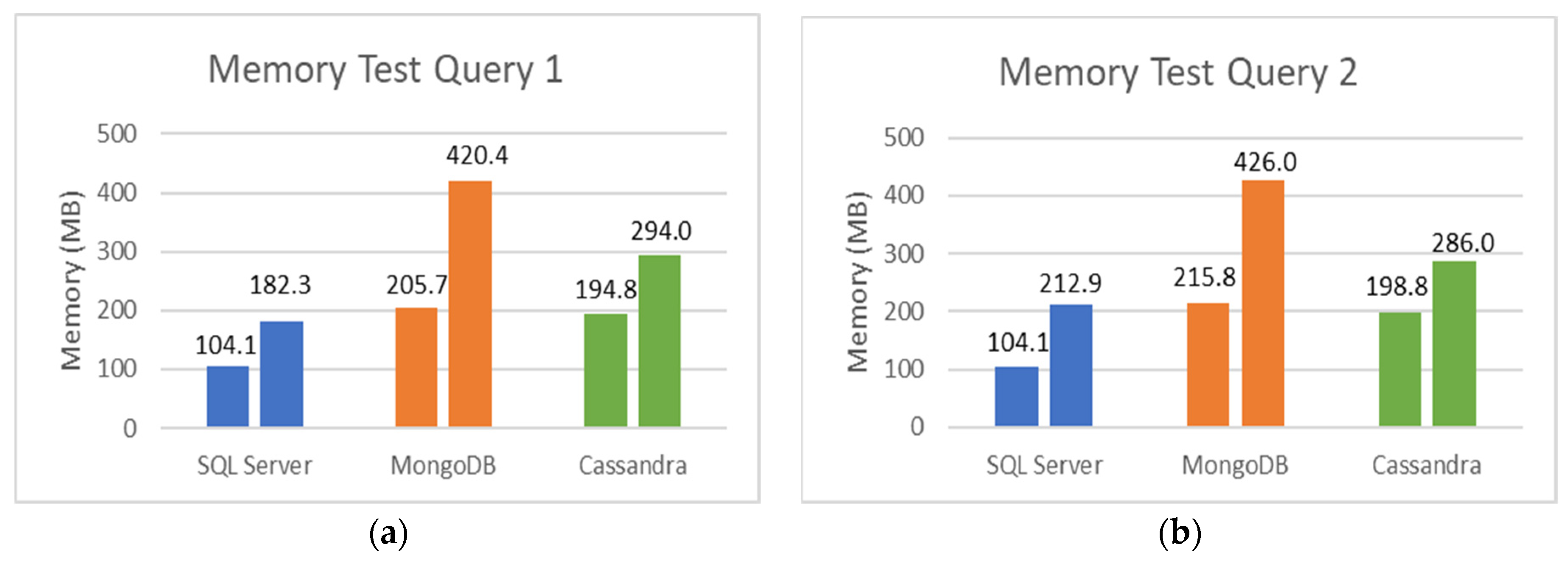
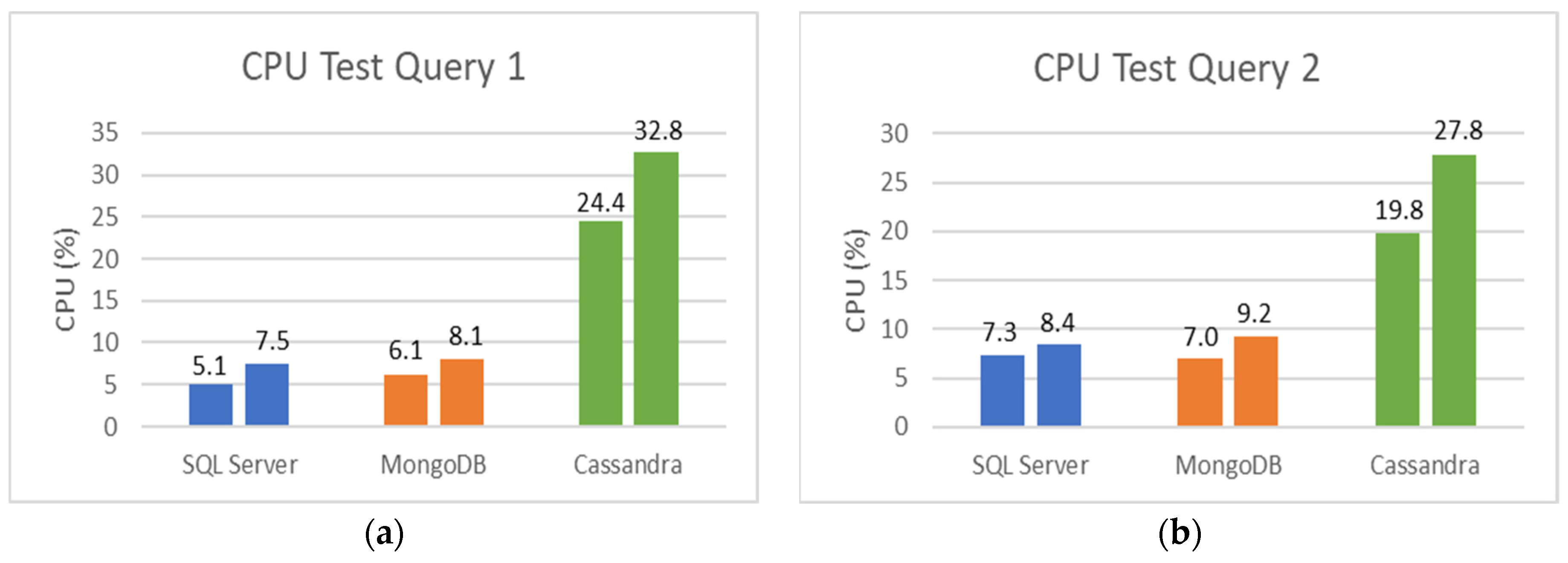
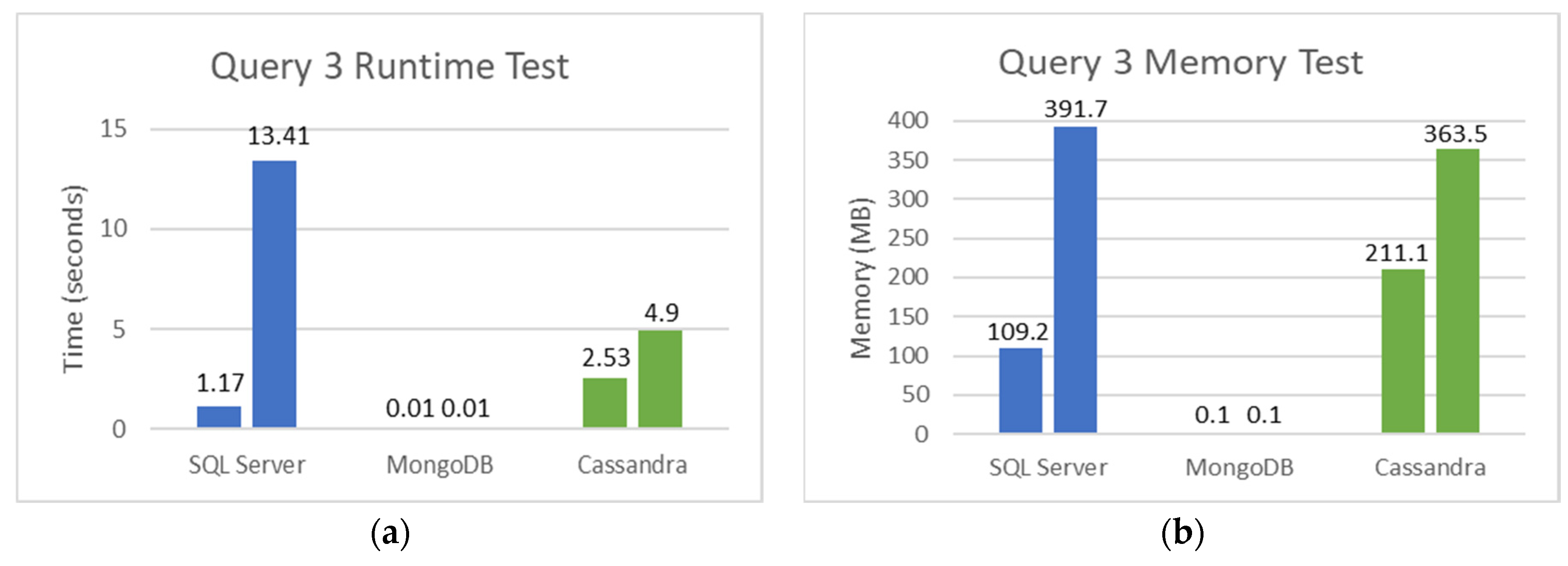
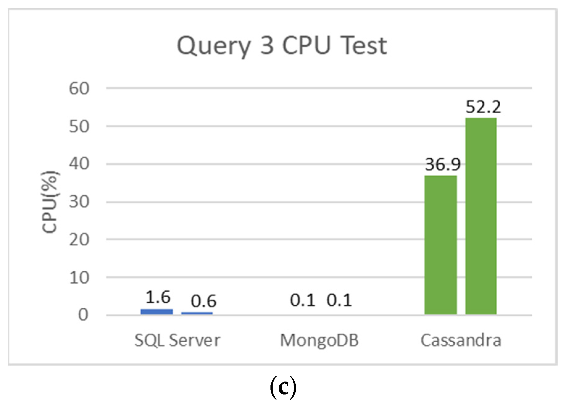
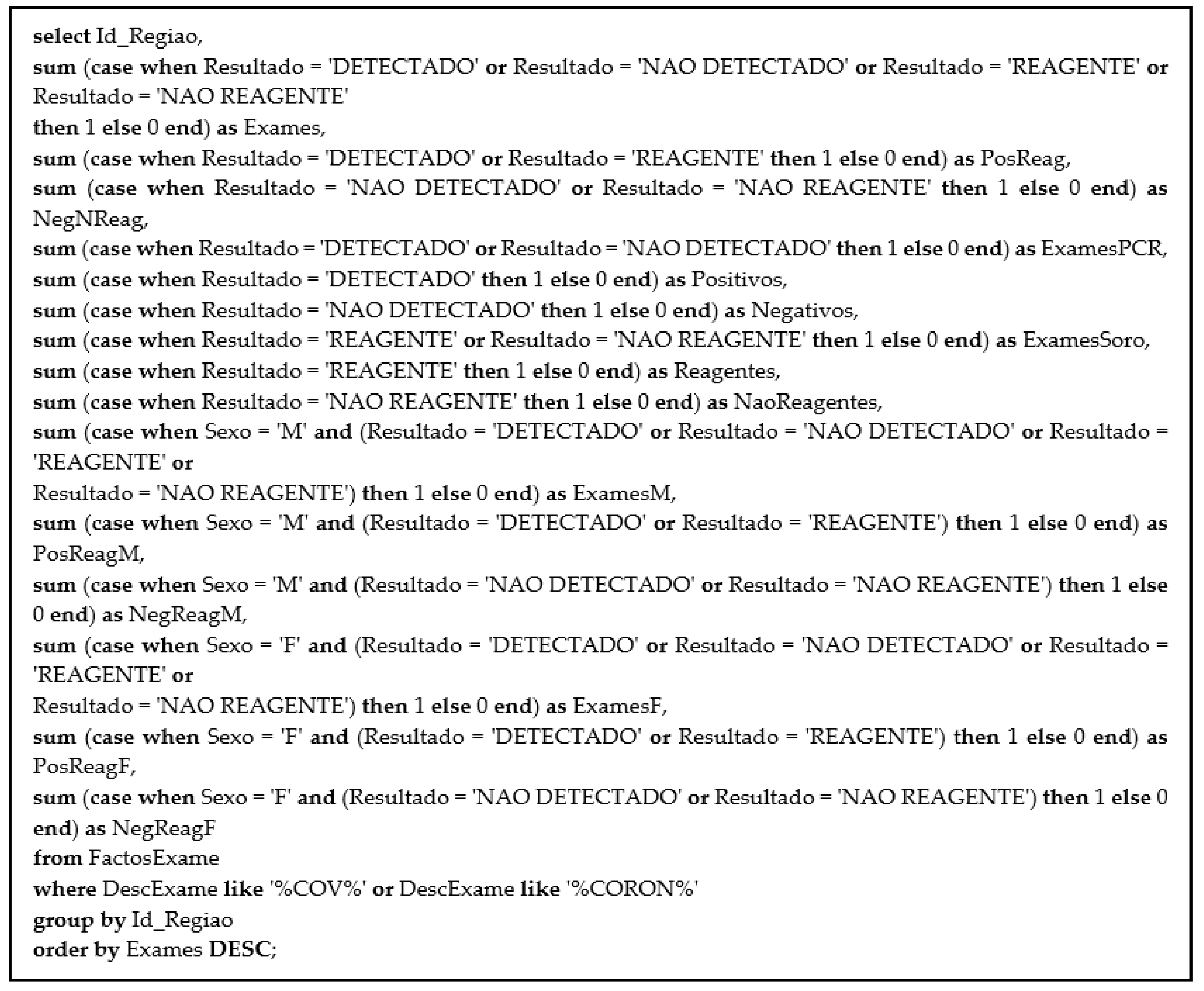
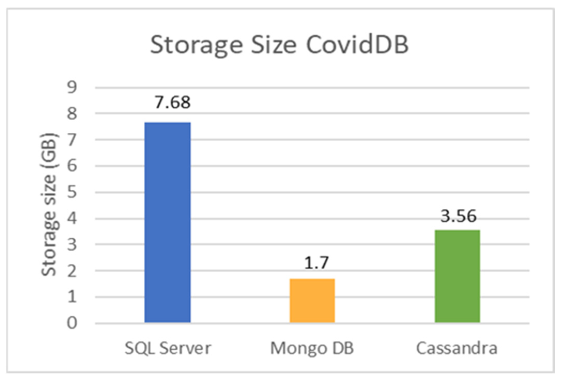
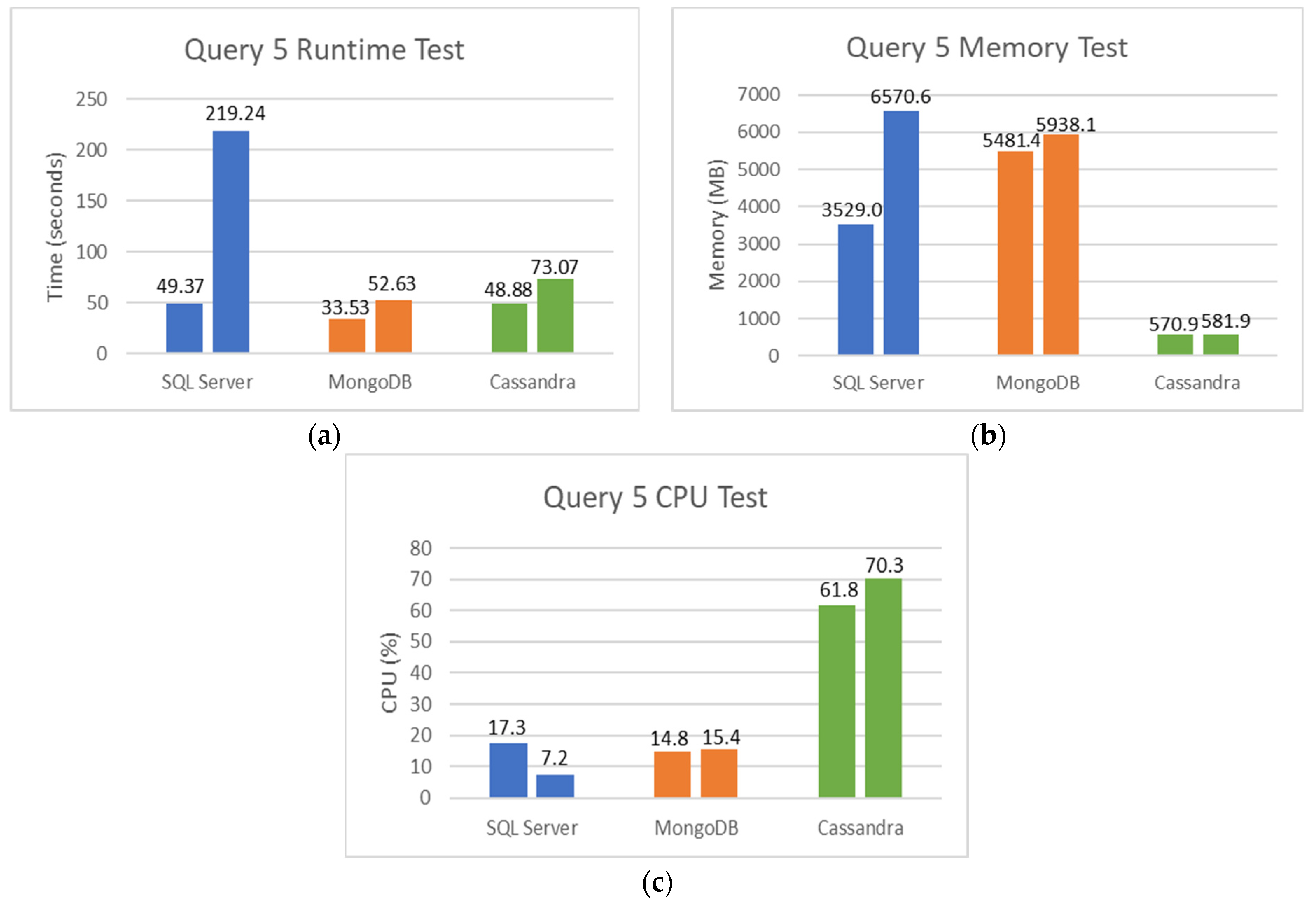
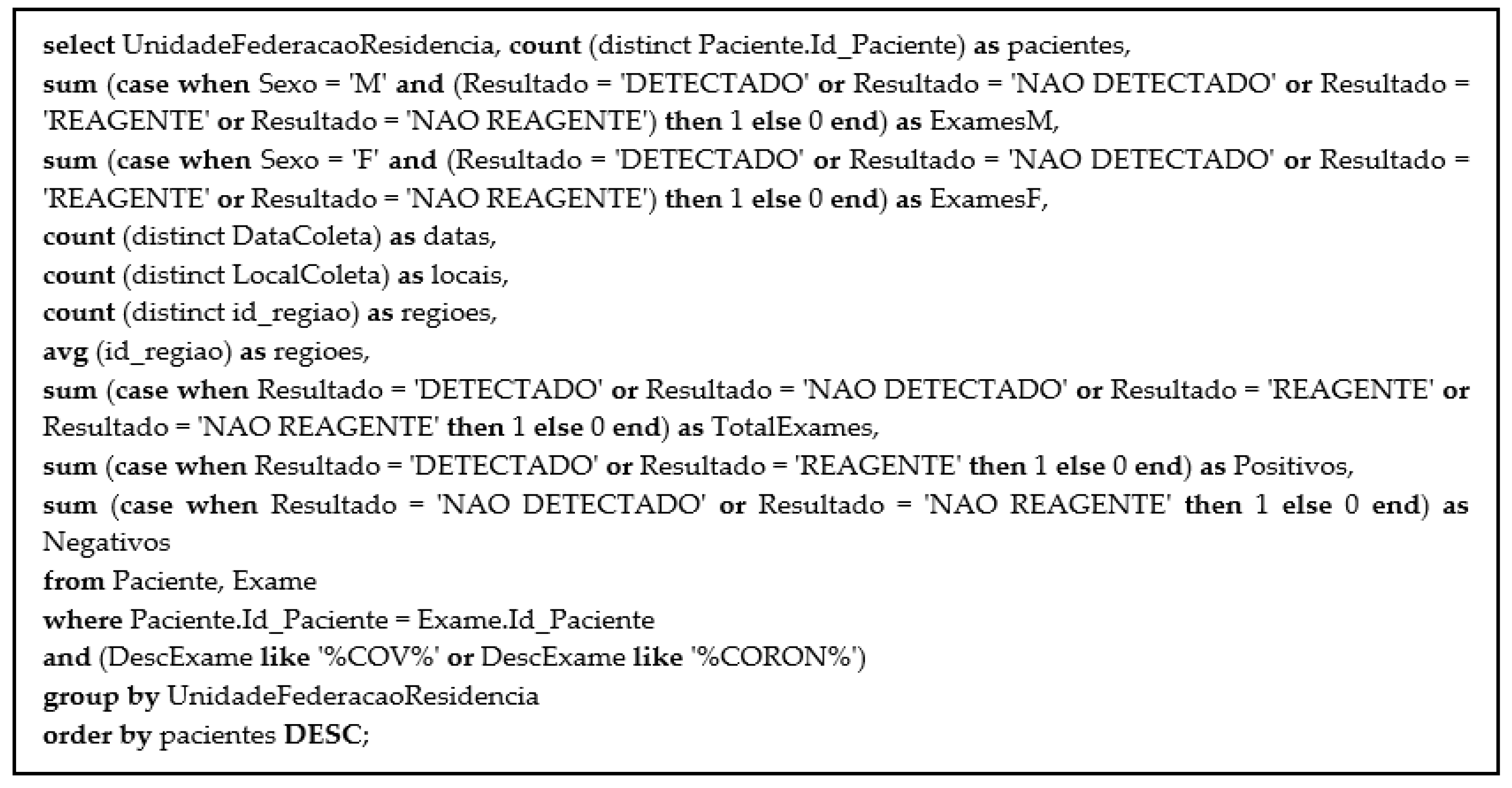
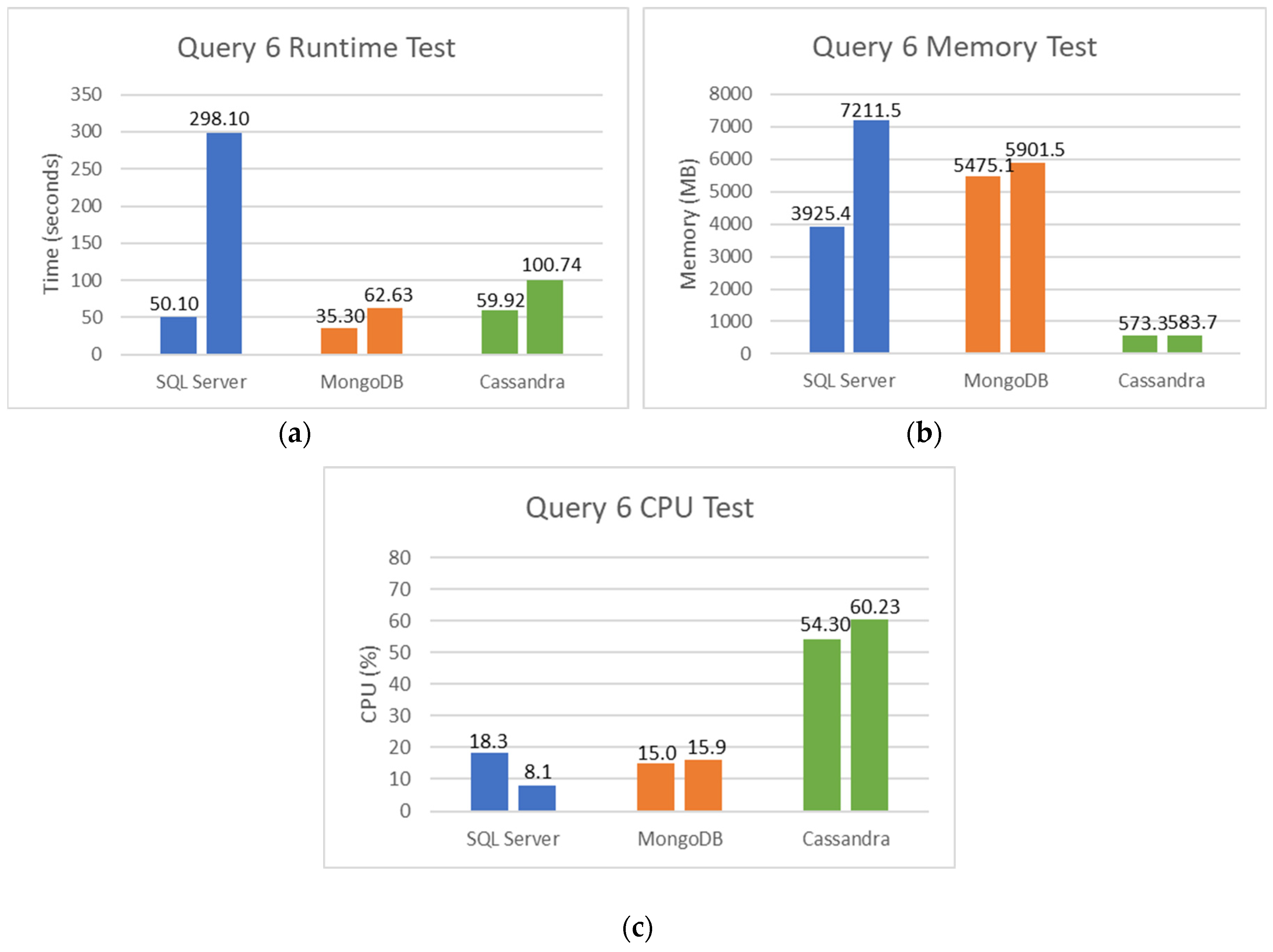
5.2. SQL and NoSQL Database Experiments
- The first set is the total counts performed for COVID-19 (PCR and serological tests): how many of these tests were detected or reactive to COVID-19 and how many were not seen or not reactive COVID-19;
- The second set is the total number of PCR tests: how many of these tests were detected by COVID-19, and how many were not seen by COVID-19;
- The third set is the total number of serological tests: how many of these tests were reactive to COVID-19, and how many were non-reactive to COVID-19;
- The fourth set is the total tests performed on male patients: how many of these tests were detected or reactive to COVID-19, and how many of these tests were not seen or not reactive to COVID-19;
- Finally, the fifth set is the total tests performed on female patients: how many of these tests were not detected or not reactive to COVID-19.
6. Conclusions and Future Work
Author Contributions
Funding
Institutional Review Board Statement
Informed Consent Statement
Data Availability Statement
Conflicts of Interest
References
- Samal, J. A Historical Exploration of Pandemics of Some Selected Diseases in the World. IJHSR 2014, 4, 165–169. [Google Scholar]
- Shi, H.; Han, X.; Jiang, N.; Cao, Y.; Alwalid, O.; Gu, J.; Fant, Y.; Zhengt, C. Radiological findings from 81 patients with COVID-19 pneumonia in Wuhan, China: A descriptive study. Lancet Infect. Dis. 2020, 20, 425–434. [Google Scholar] [CrossRef]
- World Health Organization. Corona disease 2019 (COVID-19) Situation Report—No. 67; WHO: Geneva, Switzerland, 2021. [Google Scholar]
- Leshem, E.; Wilder-Smith, A. COVID-19 Vaccine Impact in Israel and a Way Out of the Pandemic; Elsevier: Amsterdam, The Netherlands, 2021; Volume 397, pp. 1783–1785. [Google Scholar]
- Muhammad, L.J.; Islam, M.M.; Usman, S.S.; Ayon, S.I. Predictive data mining models for novel coronavirus (COVID-19) infected patients’ recovery. SN Comput. Sci. 2020, 1, 206. [Google Scholar] [CrossRef] [PubMed]
- Rohini, M.; Naveena, K.R.; Jothipriya, G.; Kameshwaran, S.; Jagadeeswari, M. A Comparative Approach to Predict Corona Virus Using Machine Learning. In Proceedings of the International Conference on Artificial Intelligence and Smart Systems (ICAIS), Coimbatore, India, 25–27 March 2021; pp. 331–337. [Google Scholar]
- Taranu, I. Data mining in healthcare: Decision making and precision. Database Syst. J. 2015, VI, 33–40. [Google Scholar]
- Orange Data Mining. Available online: https://orangedatamining.com (accessed on 1 September 2021).
- Abramova, V.; Bernardino, J.; Furtado, P. SQL or NoSQL? Performance and scalability evaluation. Int. J. Bus. Process. Integr. Manag. 2015, 7, 314–321. [Google Scholar] [CrossRef]
- Li, Y.; Manoharan, S. A performance comparison of SQL and NoSQL databases. In Proceedings of the IEEE Pacific Rim Conference, Conference on Communications and Signal Processing (PACRIM), Victoria, BC, Canada, 27–29 August 2013. [Google Scholar]
- Microsoft SQL Server 2017. Available online: https://www.microsoft.com/en-au/sql-server/sql-server-2017 (accessed on 1 September 2021).
- Mongo, D.B. Available online: https://www.mongodb.com/ (accessed on 1 September 2021).
- Cassandra. Available online: https://cassandra.apache.org/ (accessed on 1 September 2021).
- Nayak, A.; Poriya, A.; Poojary, D. Type of nosql databases and its comparison with relational databases. Int. J. Appl. Inf. Syst. (IJAIS) 2013, 5, 16–19. [Google Scholar]
- Mohamed, M.A.; Altrafi, O.G.; Ismail, M.O. Relational vs NoSQL Databases: A Survey. Int. J. Comput. Inf. Technol. 2014, 3, 598–601. [Google Scholar]
- Raut, D.A.B. NoSQL Database and Its Comparison with RDBMS. Int. J. Comput. Intell. Res. 2015, 7, 314–321. [Google Scholar]
- Chakraborty, S.; Paul, S.; Hasan, K.M.A. Performance Comparison for Data Retrieval from NoSQL and SQL Databases: A Case Study for COVID-19 Genome Sequence Dataset. In Proceedings of the International Conference on Robotics, Electrical and Signal Processing Techniques (ICREST), Dhaka, Bangladesh, 5–7 January 2021; pp. 324–328. [Google Scholar]
- Abramova, V.; Bernardino, J. NoSQL Databases: MongoDB vs Cassandra. In Proceedings of the C3S2E Proceedings of the International Conference on Computer Science and Software Engineering, Porto, Portugal, 10–12 July 2013; Association for Computing Machinery: New York, NY, USA, 2013. [Google Scholar]
- Abramova, V.; Bernardino, J.; Furtado, P. Which NoSQL Database? A Performance Overview. Open J. Databases (OJDB) 2014, 1, 17–24. [Google Scholar]
- Abramova, V.; Bernardino, J.; Furtado, P. Experimental evaluation of NoSQL databases. Int. J. Database Manag. Syst. 2014, 6, 1. [Google Scholar] [CrossRef]
- Lourenço, J.; Abramova, V.; Vieira, M.; Cabral, B.; Bernardino, J. NoSQL Databases: A Software Engineering Perspective. In New Contributions in Information Systems and Technologies Advances in Intelligent Systems and Computing; Springer: Berlin/Heidelberg, Germany, 2015; Volume 353, pp. 741–750. [Google Scholar]
- Muhammad, L.J.; Ebrahem, A.A.; Usman, S.S.; Abdulkadir, A.; Chakraborty, C.; Mohammed, I.A. Supervised Machine Learning Models for Prediction of COVID-19 Infection using Epidemiology Dataset. SN Comput. Sci. 2021, 2, 11. [Google Scholar] [CrossRef] [PubMed]
- Awadh, W.A.; Alasady, A.S.; Mustafa, H.I. Predictions of COVID-19 Spread by Using Supervised Data Mining Techniques. J. Phys. Conf. Ser. 2020, 1879, 022081. [Google Scholar] [CrossRef]
- Abdulkareem, N.M.; Abdulazeez, D.Q.; Zeebaree, D.A.H. COVID-19 World Vaccination Progress Using Machine Learning Classification Algorithms. Qubahan Acad. J. 2021, 1, 100–105. [Google Scholar] [CrossRef]
- Guzmán-Torres, J.A.; Alonso-Guzmán, E.M.; Domínguez-Mota, F.J.; Tinoco-Guerrero, G. Estimation of the Main Conditions in (SARS-CoV-2) COVID-19 Patients That Increase the Risk of Death Using Machine Learning, the Case of Mexico; Elsevier: Amsterdam, The Netherlands, 2021; Volume 27. [Google Scholar]
- Shanbehzadeh, M.; Orooji, A.; Arpanahi, H.K. Comparing of Data Mining Techniques for Predicting In-Hospital Mortality among Patients with COVID-19. J. Biostat. Epidemiol. 2021, 7, 154–169. [Google Scholar] [CrossRef]
- Keshavarzi, A. Coronavirus Infectious Disease (COVID-19) Modeling: Evidence of Geographical Signals. SSRN Electron. J. 2020. [CrossRef]
- Saire, J.E.C. Data Mining Approach to Analyze Covid-19 Dataset of Brazilian Patients. medRxiv 2020. [CrossRef]
- Thange, U.; Shukla, V.K.; Punhani, R. Analyzing COVID-19 Dataset through Data Mining Tool “Orange”. In Proceedings of the International Conference on Computation, Automation and Knowledge Management (ICCAKM), Dubai, United Arab Emirates, 19–21 January 2021; pp. 198–203. [Google Scholar]
- Bramer, M. Principles of Data Mining; Springer: London, UK, 2007. [Google Scholar]
- Fayyad, U.; Shapiro, G.P.; Smyth, P. From Data Mining to Knowledge Discover in Databases. AI Mag. 1996, 17, 37–54. [Google Scholar]
- Han, J.; Kamber, M.; Pei, J. Data Mining Concepts and Techniques, 3rd ed.; Elsevier: Waltham, MA, USA, 2006. [Google Scholar]
- Orange Data Mining Models. Available online: https://orange3.readthedocs.io/projects/orange-visual-programming/en/latest/index.html# (accessed on 1 September 2021).
- Joseph, S.I.T. Survey of data mining algorithms for intelligent computing system. J. Trends Comput. Sci. Smart Technol. (TCSST) 2019, 1, 14–23. [Google Scholar]
- Breiman, L. Random Forests. Mach. Learn. 2001, 45, 5–32. [Google Scholar] [CrossRef] [Green Version]
- Sperandei, S. Understanding logistic Regression analysis. Biochem. Med. 2014, 24, 12–18. [Google Scholar] [CrossRef] [PubMed]
- Bernardino, J.; Madeira, H. Experimental evaluation of a new distributed partitioning technique for data warehouses. In Proceedings of the 2001 International Database Engineering and Applications Symposium, Grenoble, France, 16–18 July 2001; pp. 312–321. [Google Scholar] [CrossRef]
- Bernardino, J.; Furtado, P.; Madeira, H. DWS-AQA: A cost effective approach for very large data warehouses. In Proceedings of the International Database Engineering and Applications Symposium, Montreal, QC, Canada, 14–16 July 2002; pp. 233–242. [Google Scholar] [CrossRef]
- SQL Server Integration Services. Available online: https://docs.microsoft.com/en-us/sql/integration-services/ssis-how-to-create-an-etl-package?view=sql-server-ver15 (accessed on 1 September 2021).


| Algorithm | I | II | III | IV | V | VI | Average |
|---|---|---|---|---|---|---|---|
| Random Forest | 0.928 | 0.959 | 0.961 | 0.989 | 0.996 | 0.980 | 0.9688 |
| Decision Tree | 0.924 | 0.957 | 0.961 | 0.989 | 0.996 | 0.979 | 0.9677 |
| Logistic Regression | 0.919 | 0.955 | 0.959 | 0.989 | 0.996 | 0.978 | 0.9660 |
| Naïve Bayes | 0.914 | 0.944 | 0.949 | 0.971 | 0.974 | 0.965 | 0.9528 |
| Algorithm | I | II | III | IV | V | VI | Average |
|---|---|---|---|---|---|---|---|
| Random Forest | 0.910 | 0.952 | 0.947 | 0.984 | 0.993 | 0.972 | 0.9597 |
| Decision Tree | 0.908 | 0.949 | 0.923 | 0.979 | 0.992 | 0.959 | 0.9517 |
| Logistic Regression | 0.894 | 0.947 | 0.947 | 0.984 | 0.993 | 0.971 | 0.9560 |
| Naïve Bayes | 0.890 | 0.942 | 0.956 | 0.986 | 0.994 | 0.976 | 0.9573 |
| Algorithm | I | II | III | IV | V | VI | Average |
|---|---|---|---|---|---|---|---|
| Random Forest | 0.919 | 0.953 | 0.947 | 0.984 | 0.994 | 0.972 | 0.9615 |
| Decision Tree | 0.916 | 0.947 | 0.941 | 0.984 | 0.994 | 0.969 | 0.9585 |
| Logistic Regression | 0.900 | 0.949 | 0.950 | 0.985 | 0.994 | 0.974 | 0.9587 |
| Naïve Bayes | 0.900 | 0.943 | 0.952 | 0.978 | 0.983 | 0.970 | 0.9543 |
| Algorithm | VII | VIII | IX | X | XI | XII | XIII | XIV | Average |
|---|---|---|---|---|---|---|---|---|---|
| Random Forest | 0.896 | 0.900 | 0.920 | 0.924 | 0.912 | 0.895 | 0.890 | 0.917 | 0.9068 |
| Decision Tree | 0.896 | 0.900 | 0.919 | 0.924 | 0.912 | 0.895 | 0.890 | 0.917 | 0.9066 |
| Logistic Regression | 0.890 | 0.894 | 0.913 | 0.917 | 0.908 | 0.889 | 0.889 | 0.912 | 0.9015 |
| Naïve Bayes | 0.893 | 0.893 | 0.909 | 0.913 | 0.902 | 0.891 | 0.885 | 0.907 | 0.8991 |
| Algorithm | VII | VIII | IX | X | XI | XII | XIII | XIV | Average |
|---|---|---|---|---|---|---|---|---|---|
| Random Forest | 0.876 | 0.866 | 0.897 | 0.904 | 0.887 | 0.871 | 0.846 | 0.889 | 0.8795 |
| Decision Tree | 0.876 | 0.866 | 0.897 | 0.904 | 0.887 | 0.871 | 0.846 | 0.889 | 0.8795 |
| Logistic Regression | 0.856 | 0.851 | 0.878 | 0.886 | 0.873 | 0.850 | 0.844 | 0.874 | 0.8640 |
| Naïve Bayes | 0.867 | 0.867 | 0.884 | 0.891 | 0.872 | 0.862 | 0.851 | 0.879 | 0.8761 |
| Algorithm | VII | VIII | IX | X | XI | XII | XIII | XIV | Average |
|---|---|---|---|---|---|---|---|---|---|
| Random Forest | 0.884 | 0.877 | 0.906 | 0.913 | 0.897 | 0.880 | 0.862 | 0.903 | 0.8903 |
| Decision Tree | 0.884 | 0.877 | 0.906 | 0.913 | 0.897 | 0.880 | 0.862 | 0.903 | 0.8902 |
| Logistic Regression | 0.868 | 0.867 | 0.888 | 0.895 | 0.887 | 0.865 | 0.862 | 0.890 | 0.8778 |
| Naïve Bayes | 0.877 | 0.879 | 0.896 | 0.901 | 0.885 | 0.875 | 0.866 | 0.892 | 0.8839 |
Publisher’s Note: MDPI stays neutral with regard to jurisdictional claims in published maps and institutional affiliations. |
© 2022 by the authors. Licensee MDPI, Basel, Switzerland. This article is an open access article distributed under the terms and conditions of the Creative Commons Attribution (CC BY) license (https://creativecommons.org/licenses/by/4.0/).
Share and Cite
Antas, J.; Rocha Silva, R.; Bernardino, J. Assessment of SQL and NoSQL Systems to Store and Mine COVID-19 Data. Computers 2022, 11, 29. https://doi.org/10.3390/computers11020029
Antas J, Rocha Silva R, Bernardino J. Assessment of SQL and NoSQL Systems to Store and Mine COVID-19 Data. Computers. 2022; 11(2):29. https://doi.org/10.3390/computers11020029
Chicago/Turabian StyleAntas, João, Rodrigo Rocha Silva, and Jorge Bernardino. 2022. "Assessment of SQL and NoSQL Systems to Store and Mine COVID-19 Data" Computers 11, no. 2: 29. https://doi.org/10.3390/computers11020029
APA StyleAntas, J., Rocha Silva, R., & Bernardino, J. (2022). Assessment of SQL and NoSQL Systems to Store and Mine COVID-19 Data. Computers, 11(2), 29. https://doi.org/10.3390/computers11020029