Article

Implementation of a C Library of Kalman Filters for Application on Embedded Systems

Institute of System Dynamics and Control, Robotics and Mechatronics Center, German Aerospace Center (DLR), 82234 Weßling, Germany
*
Author to whom correspondence should be addressed.
Computers 2022, 11(11), 165; https://doi.org/10.3390/computers11110165
Submission received: 14 October 2022 / Revised: 10 November 2022 / Accepted: 14 November 2022 / Published: 18 November 2022
(This article belongs to the Special Issue Real-Time Embedded Systems in IoT)

Abstract

:
Having knowledge about the states of a system is an important component in most control systems. However, an exact measurement of the states cannot always be provided because it is either not technically possible or only possible with a significant effort. Therefore, state estimation plays an important role in control applications. The well-known and widely used Kalman filter is often employed for this purpose. This paper describes the implementation of nonlinear Kalman filter algorithms, the extended and the unscented Kalman filter with square-rooting, in the programming language C, that are suitable for the use on embedded systems. The implementations deal with single or double precision data types depending on the application. The newly implemented filters are demonstrated in the context of semi-active vehicle damper control and the estimation of the tire–road friction coefficient as application examples, providing real-time capability. Their per-formances were evaluated in tests on an electronic control unit and a rapid-prototyping platform.

1. Introduction

In control engineering applications, such as vehicle dynamics control, it is crucial to identify the states of a system as precisely as possible. In some cases, the states can be measured by means of appropriate sensors, such as accelerometers for determining the acceleration of a vehicle tire. However, such sensors are not always available for technical or economic reasons. This means that it might not be technically possible to measure a state because of suitable sensor absence, too-high costs, or too-complex incorporation. One possibility to gain knowledge about the states of a system is to estimate them. This approach uses information about the system described by a model and about system measurements in order to determine the states of interest. A well-established and wide-spread state estimation technique is Kalman filtering. This technique is based on a recursive estimation of the current states using the estimated states of the previous step and the new measurements [1]. The popularity of the Kalman filter is due to its capabilities of predicting the state for the next time step and filtering out noise in the measurements, and its easier implementation compared to other state estimation techniques [2]. Although the basic Kalman filter is applied to linear systems, there are also several variants with extensions of the filter algorithm to handle nonlinearities.

1.1. Application Fields of Kalman Filtering

Kalman filters have applications in numerous fields. The unscented Kalman filter, for example, is used in [3] for target tracking. A combination of a convolutional neural network and a Kalman filter is used in [4] for detecting and tracking the motion of pigs in a video with the aim of determining social interactions. The extended Kalman filter is applied for the localization of a mobile robot that is provided with multiple sensors in [5]. The latter variant is also employed in a similar field in [6], together with the Kalman filter, within a localization and mapping algorithm to measure the position of a robot. A five-state extended Kalman filter is designed in [7], estimating the speed over the ground of an unmanned surface vehicle, in addition to other quantities needed for course control, and experimental results are shown. In [8], a lithium-ion battery cell is modeled and a state of charge estimation is carried out. An algorithm for pose estimation based on one or several event-based sensors is presented in [9], incorporating an extended Kalman filter that is real-time capable in the case of one sensor.

1.2. Embedded Implementation of Kalman Filter Algorithms

When working with road vehicles, robots, or flying devices, it becomes necessary to implement state estimators on embedded systems that are incorporated in them. This allows processes to be executed in real time. In [10], a simple 1-D Kalman filter is used to attenuate noise of the measured accelerations of an unmanned aerial vehicle and is executed in real time on a microcontroller. The authors of [11] implement an unscented Kalman filter for data fusion on navigation systems. Therein, the authors choose two microcontrollers and present platform-dependent modifications along with general customizations in the filter algorithms. A C library for an embedded extended Kalman filter is proposed in [12], representing a small implementation usable also for the linear Kalman filter. In [13], a detailed approach to deriving data fusion of smart sensors using Kalman filters is developed and the complexities of different filter variants are compared. Finally, the estimation applied to a 2-D orientation problem is carried out, using a C implementation on a microcontroller.
The implementation of state estimators gains special importance, since some requirements on the program code have to be fulfilled. Real-time capability demands that the program provides a solution within a certain fixed period of time, the specific length of which depends on the application. Due to limited resources on the embedded system, a narrower floating-point data type is used compared to desktop implementations, for example, 32-bit instead of 64-bit precision. The software must be able to yield sufficiently good results even with this limited number of bits [14]. Furthermore, on an embedded system, dynamic memory allocation cannot be used. In addition, the software must consist of self-contained code that does not require any other external libraries. On embedded systems, the programming language C is widely used. A state estimator implemented fully standalone and manually in C entails the advantages of this language. It is also possible to generate C code from other programming languages using appropriate tools, but, in general, manually written code can provide the additional benefits of better readability and maintainability, and no unnecessary code overhead is imposed. Another requirement associated with the use of software in embedded and, especially, safety-critical applications, is adherence to coding guidelines such as MISRA C [15]. The fulfillment of these rules is often postulated in the automotive sector and also in other industries [16].

1.3. Contribution of This Work

Considering this framework, this paper presents a newly implemented Kalman filter library that is suitable for use on embedded systems. It is written in C code and represents a stand-alone library without the need for any external libraries. Some numerical routines used inside the estimation algorithms are based on existing Fortran routines of the widely known Linear Algebra Package (LAPACK) [17], but reimplemented in C. The new library contains two variants of nonlinear Kalman filters that were implemented in a numerically efficient way. It supports 64-bit and 32-bit setups, suiting the limited resources on embedded systems. The implementation incorporates common coding guidelines. The Kalman filter library is successfully utilized in vehicle state estimation in two different application scenarios and integrated and validated in real-time embedded environments.
The introduced library represents an in-house development and is used internally for research projects. It is not currently planned to make it publicly available, though interested readers may contact the authors.
The Kalman filter theory is explained in Section 2. Section 3 covers the implementation of the new library, including the general structure, the integration of user-defined prediction models, basic numerical routines, and the consideration of coding guidelines. In Section 4, the applications of the library on an electronic control unit (ECU) and a rapid prototyping platform are described and validations are carried out. Section 5 presents a conclusion.

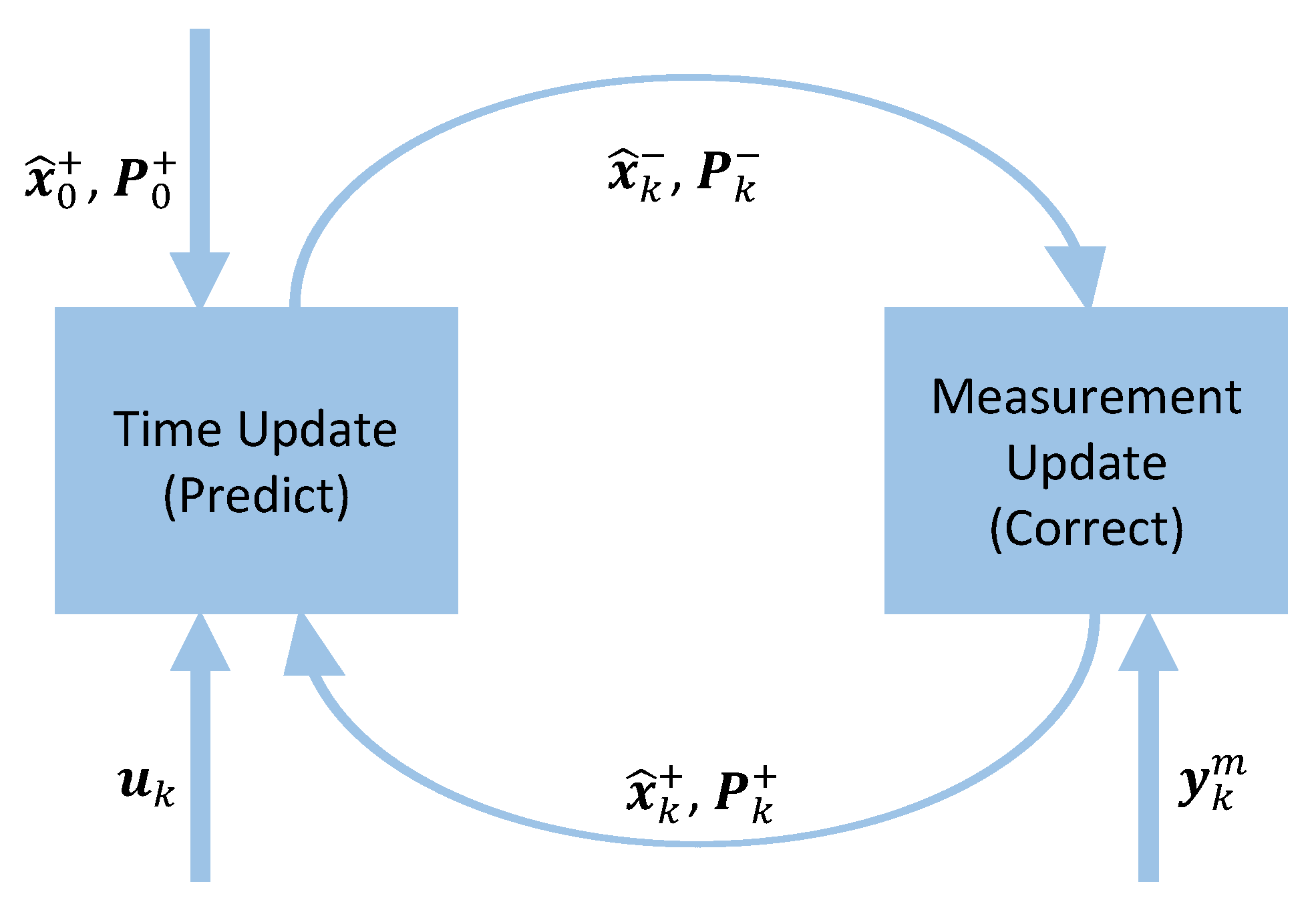
2. General Theory on Kalman Filters

This section briefly summarizes the principles for state estimation using the well-known Kalman filter. Basic theory can be found in [1,18,19]. The following notations are adapted from [20].
The subsequent nonlinear system is the basis for the state estimation. It represents the continuous-time plant model in state space form:
x ˙ = f ( x , u ) , y = h ( x ) ,
with the vector of states x ( t ) n x , the time t , the vector of inputs u ( t ) n u , the vector of outputs y ( t ) n y , and their respective dimensions n x , n u and n y . Since the aim is to implement Kalman filter algorithms for state estimation on embedded systems, which represent sampled data systems, model (1) cannot be used directly. Instead, it is transformed to a discrete-time formulation. This resulting dynamic system with additive Gaussian noise is utilized in the following discrete-time state estimation:
x k = f k | k 1 ( x k 1 , u k 1 ) + w k 1 , y k = h ( x k ) + v k , w k   ~   N ( 0 , Q ) , v k   ~   N ( 0 , R ) ,
with x k = x ( t k ) , u k = u ( t k ) and y k = y ( t k ) , where t k denotes the k-th sample time point in a data system sampled periodically. Both the system and output formulas are perturbed by white Gaussian noises w k and v k . They are assumed to be uncorrelated with zero mean. The corresponding covariance matrices for the noises are described by Q and R , which are regarded to be constant. The discrete-time integration between the last sample point t k 1 and the new one t k is described by the following equation:
f k | k 1 = x k 1 + t k 1 t k f ( x , u k 1 ) d t ,
whereby the integration can be performed by using, e.g., Runge-Kutta or Euler methods. The required evaluations of the prediction model in the Kalman filter algorithms are described by (1) and (3).
Figure 1 shows the basic idea of state estimation using Kalman filtering, see also [20].
A recursive algorithm is presupposed, which consists of the two steps predict and correct, building a cyclic flow. At the beginning, the filter is initialized with x ^ 0 + and P 0 + , which is an initial estimate for the state vector and the state covariance matrix, that indicates the confidence in this first guess. The first step of the cycle in Figure 1 refers to the predict step. It represents an a priori estimation of the mean and covariance, which means a gauge for the trust in the system states. The outcomes of this step have a “−” in their superscripts in the following. This is succeeded by the correct step, the results of which have a “+” in the superscript. In this step, the covariance matrix and the estimated states are updated, using the calculated Kalman gain and the current measurements of the outputs y k m in the actual sample k . Afterwards the predict step follows and the procedure repeats with k : = k + 1 . The cycle is carried out with a specified sample time T s . At every sample period, new measurements of the outputs are provided and used to update the current estimation of the states.

2.1. Nonlinear Kalman Filter Variants

Based on this general principle of state estimation, there are several variants of Kalman filters. The pure Kalman filter is suited for linear systems. However, real-world systems often include nonlinearities. In order to be able to also apply the state estimation to these systems, nonlinear Kalman filters were developed, for example, the extended Kalman filter (EKF) and the unscented Kalman filter (UKF). Since these two variants are well known and widely used, only a short overview is given at this point for the sake of brevity. A detailed description of the algorithms of both variants can be found in Appendix A.
The EKF linearizes the model using Taylor series expansions, while the UKF does not use approximations for performing state estimation on nonlinear systems. Instead, it selects specified points, the sigma points, around the current states and propagates them through the nonlinear function of the system to estimate the next state. As a result, the UKF has a higher accuracy compared to the EKF. However, its implementation requires higher computational effort.
As an extension to the EKF and the UKF in terms of numerical robustness, there are also the extended Kalman filter with square-rooting (EKF-SR) and the unscented Kalman filter with square-rooting (UKF-SR). These two variants use a decomposition of the state covariance matrix and employ its positive definiteness, entailing higher numerical stability of the square-rooting (SR) variants compared to the original filters.
The filter equations of the EKF and the EKF-SR are summarized in Section A.1 and Section A.2, respectively. The UKF and its modifications to the UKF-SR are described in Section A.3 and Section A.4.

2.2. Incorporation of State Constraints

As an augmentation to the methods of state estimation with Kalman filtering described above, it is also possible to consider additional constraints on the states. This may be essential in some practical applications where physical limitations on the states are imposed. These include, for example, the need for positive concentrations in a chemical system. Taking this additional information about the constraints into account, the estimation of the states becomes more reliable. An approach to realize this with the UKF is suggested in [21]. Therein, the inequality constraints define a feasible range for the states. If sigma points for the UKF are outside this range, they are projected to the edge of the admissible region. This is applied directly after the computation of the sigma points in Equation (A10) and again after their propagation through the nonlinear function in Equation (A11). The same method is employed for the estimated states if they do not respect the constraints. Using the described approach of projecting the sigma points, the constraints also affect the covariance. In contrast to simply clipping the estimated states, this makes the estimation more precise. This state constraint method thus provides additional support for the estimation so that physically infeasible state values do not occur at all. In [20] an overview of methods for handling constraints in state estimation is provided.

3. Implementation of the Embedded Kalman Filter Library

The embedded Kalman filter library comprises implementations for the EKF-SR and the UKF-SR. It is based on an internally developed library; see [22,23]. In contrast, all parts of the embedded Kalman filter library were newly implemented in C without dependencies on external libraries.
This section presents details about the implementation of the embedded Kalman filter library. Its general structure is shown, in addition to its usage with user-defined prediction models. Additionally, a summary of the employed numerical routines is given and features of the implementation regarding coding guidelines are described.

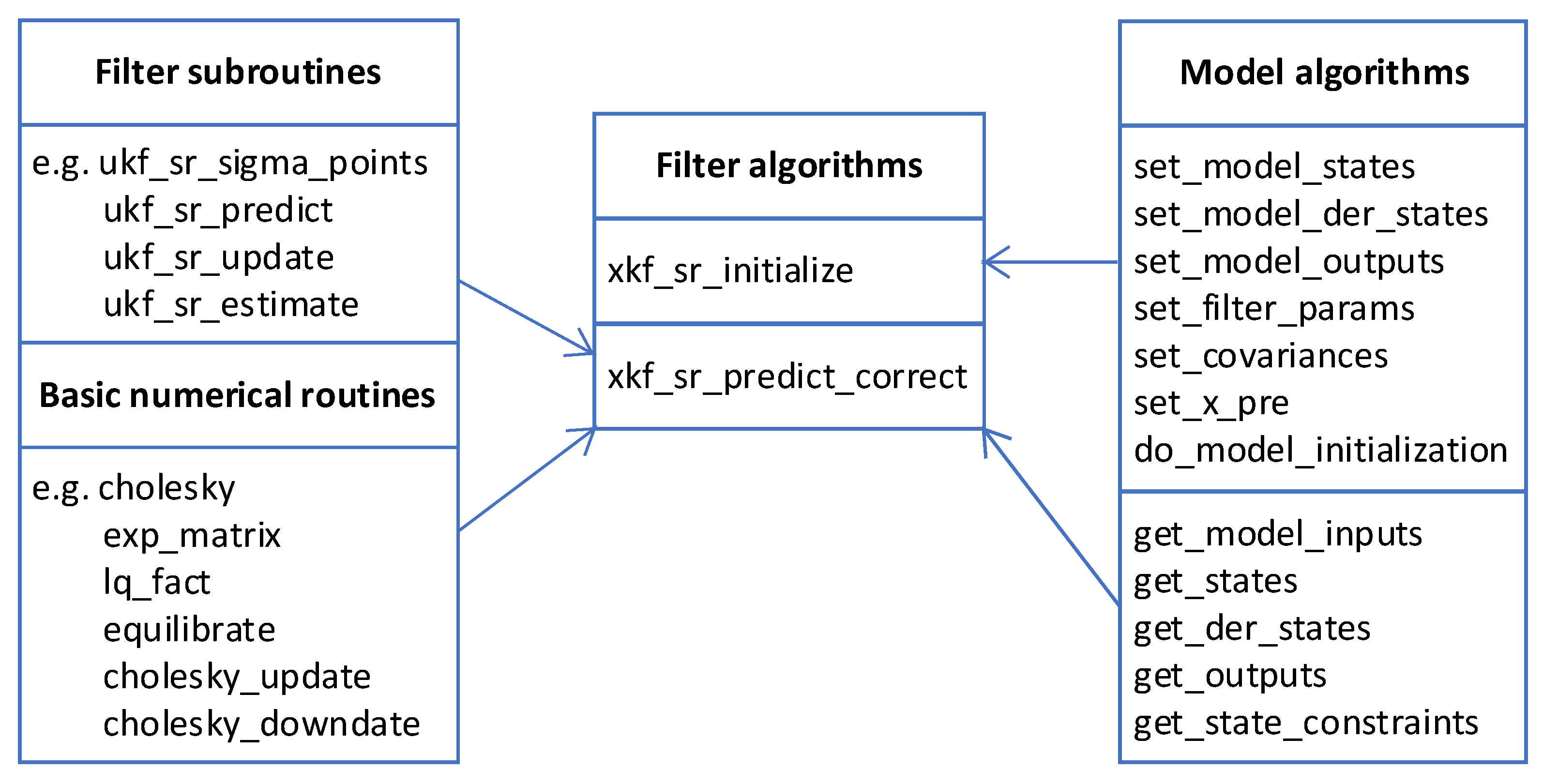
3.1. Structure of the Embedded Kalman Filter Library

The library is generally composed of generic filter parts and model-specific parts. The filter parts contain the routines of the respective filter variant including all necessary numerical routines, but do not hold any prediction model-specific information. These are grouped in a separate part of the library. Therefore, the generic filter parts can be applied without any problem-specific adaptations. Figure 2 shows the general structure of the library, with the generic filter parts on the left side and the model-specific parts on the right.
The filter algorithms (see the middle part of Figure 2) are divided into an initialization part and a main part. The corresponding functions are named xkf_sr_initialize and xkf_sr_predict_correct, where the prefix depends on the respective filter variant, i.e., ekf_sr or ukf_sr. In the function xkf_sr_predict_correct the actual evaluation of the Kalman filter routines takes place. Here, the computations for the time and measurement update, the predict and correct steps, are carried out, see Figure 1. The specific operations depend on the filter variant used and are listed in the appendix in Table A1 and Table A5, respectively in the modifications (A22)–(A25). Thus, the function xkf_sr_predict_correct constitutes the cyclic flow of the filter algorithms and is executed in each time step of the estimation. It utilizes the inputs u k of the prediction model as well as the measured model outputs y k m . The output of the function represents the estimated states x ^ k + to be computed by the filter algorithm at sample time t k , cf. Figure 3 for illustration.
To include the embedded Kalman filter library in a given software environment for a known prediction model, the user needs
  • to provide prediction model-specific functions using the given interfaces of the library (right part of Figure 2), see Section 3.2 for more details on these functions,
  • to call the function xkf_sr_initialize once in the initialization phase,
  • to call the function xkf_sr_predict_correct in each sample time step of the environment, and
  • to provide variables for the inputs u k , y k m and the outputs x ^ k + of the function xkf_sr_predict_correct.
The filter algorithm functions have the following C prototypes:
  • void xkf_sr_initialize (void)
  • void xkf_sr_predict_correct (real_t * ptr_u, real_t * ptr_y_meas, real_t * ptr_out)
In the routine xkf_sr_initialize, all global variables are initialized and the model-specific initialization functions are called, for example for setting the filter parameters, providing an initial guess for the states and for initializing the model variables.
The function parameters of xkf_sr_predict_correct must be set in the software environment before the first call. They represent pointers to variables for the inputs u k (ptr_u) and measured outputs y k m (ptr_y_meas) of the prediction model and the estimated states x ^ k + (ptr_out). In the function, several model-specific functions are called in a generic way, for example to perform the model evaluations from (1) and (3). Further, filter subroutines and basic numerical routines are employed, see left part of Figure 2. More details on the latter functions are given in Section 3.3. The filter subroutines carry out the respective filter computations, see Appendix A, e.g., ukf_sr_sigma_points performs (A10).
The data type named real_t is defined in the library and used for single or double precision floating-point variables. By doing this, the whole library is available in both a float 32-bit and a float 64-bit configuration, where the switch is done by simply activating a macro in the code. Thus, depending on the application, the data type and the desired accuracy can be selected. For example, offline simulations with the purpose of validating the estimation may need a higher accuracy, whereas the use on embedded systems requires single precision computing. The model code needs to support the use of this data type real_t or to provide another data type that is suitable for the chosen precision, i.e., 32-bit or 64-bit.

3.2. Incorporation of User-Defined Prediction Models

It is presupposed that the prediction model whose states are to be estimated is available as C code, including the model evaluations from (1) and (3). For example, this can be accomplished by exporting code from a simulation environment in which the model is designed. The obtained model code then needs to be interfaced to the model-specific part of the embedded Kalman filter library, see the right side of Figure 2 for the list of functions. For each prediction model, all the problem-specific information (functions, global data and macros) can be included in a single separate C file. Some functions are only needed by a certain filter variant, others by all of them.
The memory concept of the library consists of a set of global variables to be used in the generic filter functions xkf_sr_initialize or xkf_sr_predict_correct and global variables in the model-specific part. The size of the generic global arrays depends on the dimensions of the problem considered, namely the number of states n x and the number of outputs n y of the underlying model. These sizes must be defined in the model-specific part via macros NX and NY. A working memory for temporary data is also provided as a global variable and used for internal calculations in the filter subroutines and basic numerical routines. A further important part of the memory concept is global variables for the model inputs u k , the states x k , the state derivatives x ˙ k and the ouputs y k to be declared in the model-specific code and to be used in the model functions. In the following description of the model functions it is assumed that these global variables exist.
In the initialization phase of the state estimation, i.e., in the function xkf_sr_initialize, the following functions being part of the model algorithms are called first:
  • void set_model_states(real_t * states[NX])
  • void set_model_der_states(real_t * der_states[NX]) (only needed for the EKF-SR)
  • void set_model_outputs(real_t * outputs[NY])
These three functions are used to establish a link between the generic filter functions and the global model variables for states, state derivatives and outputs used in the model code. The idea is not to use the global model variables by their names but access them in the generic filter functions via vectors of pointers (states, der_states, outputs). The length of these vectors is defined by using the macros NX and NY. The vectors are provided by the function xkf_sr_initialize and their components have to be assigned in the listed functions to the memory location of the respective global model variables.
Next, the following functions are called in the initialization phase:
  • void set_x_pre(real_t xpre[NX])
  • void set_filter_params(real_t *alpha, real_t *beta, real_t *kappa) (only needed for the UKF-SR)
  • void set_covariances(real_t CfPpre[NX*NX], real_t CfQ[NX*NX], real_t CfR[NY*NY])
  • void do_model_initialization(void)
In the first function, values for the initial guess of the states x ^ 0 have to be provided. The second function is only needed for the filter variant UKF-SR and specifies the parameters α , β and κ from Table A2. In the third function, an initial estimate for the state covariance matrix P 0 and the process and measurement noise covariance matrices Q and R is set. Throughout the C program, matrices are stored column-wise via arrays and are manipulated accordingly. These three functions apply global variables as function parameters that are supplied by generic filter functions. The last function of the model-specific part that is called in xkf_sr_initialize is do_model_initialization. Here, the initialization of the underlying prediction model is performed, for example by executing a corresponding function from the user provided model code.
In the cyclically processed function xkf_sr_predict_correct, several functions from the model algorithms are also called. Concerning the model inputs u k , that arrive in each sample time step t k , that is:
  • void get_model_inputs(real_t *ptr_u)
This function is used to pass the inputs ptr_u provided by the software environment to the respective inputs of the model code.
In the further processing of xkf_sr_predict_correct, the following functions of the model algorithms are called:
  • void get_der_states(void) (only needed for the EKF-SR)
  • void get_outputs(void)
  • void get_states(void)
  • void get_state_constraints (int state_constr_ind[NX_CONSTR], real_t constrVecLow[NX_CONSTR], real_t constrVecUp[NX_CONSTR]) (optional)
By executing the first three functions the model evaluations from (1) and (3) are carried out. These are the evaluation of the state derivatives, outputs, or the updating of the states by performing the integration between two sample points.
The last function get_state_constraints denotes an optional function. If state constraints are present, they can be specified here. The function will only be activated if the user has enabled a macro and the state constraints are then incorporated in the filter algorithms as described in Section 2.2. It is possible to provide constraints for only some of the total n x states. If a state has constraints, both lower and upper constraints must be indicated. The user needs to define a macro (NX_CONSTR) for the number of states that have constraints and to give the indices of these states via the array state_constr_ind. The respective constraints are then specified in constrVecLow and constrVecUp which are provided with the appropriate length of constrained states defined by the macro.
In addition to all these mentioned model algorithms, the function xkf_sr_predict_correct executes the predict and correct steps of the respective filter variants, which do not contain any model-specific components. The functions utilized in this regard usually receive arrays as parameter arguments.
At the end of the function xkf_sr_predict_correct, the variables for the states and the system covariance matrix are set to the respective current estimates and, thus, provide the starting point for the next iteration step. The estimated states x ^ k + , representing the outputs of the main function xkf_sr_predict_correct, are passed to the surrounding software environment where the estimator is employed and where they can be further processed.

3.3. Basic Routines Employed in the Library

Most of the basic numerical routines that are used inside the generic filter functions (see left part of Figure 2) are based on LAPACK [17]. This is a well-known and established library for computations in numerical linear algebra, written in the programming language Fortran. The routines employed here include efficient vector-scalar, matrix-vector and matrix-matrix operations. Furthermore, computational routines for general matrices are used, such as an LQ factorization of a real matrix. For the embedded Kalman filter library, the mentioned numerical routines have not been used directly from LAPACK. Instead, they constituted the basis for a complete reimplementation in the programming language C. This approach ensures that no external libraries are used and that all routines are available in C.
The newly written routines incorporate details of an efficient implementation from LAPACK, for example the specification of the leading dimension of an array. This parameter enables operating with submatrices of a larger matrix. In the embedded Kalman filter library, a two-dimensional matrix is stored column-wise in a one-dimensional array. By means of the leading dimension, submatrices in larger arrays can be addressed and routines can be called with submatrices. To identify the submatrix in the whole array, four parameters are required. These are the numbers of the rows and columns of the submatrix, a pointer that defines the first element of the submatrix, and the leading dimension to find the starting point of the elements of the next column of the submatrix in the whole array. In the case of column-wise storage, the leading dimension equals the number of rows of the full matrix.
There are basic matrix operations from linear algebra that are used as essential elements in this embedded Kalman filter library. Some are applied in every filter variant, such as the Cholesky factorization, and some are employed only in one variant, such as the matrix exponential within the EKF-SR. The following main linear algebra routines are used in the library (their names in the code are given in brackets, see also Figure 2):
  • Cholesky factorization (cholesky):
    A = G G T , where A n × n is a symmetric and positive definite matrix and G n × n is a lower triangular matrix with positive diagonal entries.
    G is called the Cholesky factor. The algorithm is described in [24]. It is possible to organize the calculations in such a way that the matrix A is overwritten. Thus, no additional memory is required. The algorithm returns the lower triangle, with the remaining matrix completed with zeros. This factorization is used to obtain the matrix square-roots of the covariance matrices, see e.g., Section A.3.
  • Matrix exponential (exp_matrix):
    e A t = k = 0 ( A t ) k k ! = I + A t + ( A t ) 2 2 + ( A t ) 3 6 + , with a real matrix A n × n , the identiy matrix I and a scalar t which is the sampling time here. The computation is performed by means of a Taylor series expansion. The implementation, which is employed in Equation (A3), is based on the algorithm used in the Modelica Standard Library (“Modelica.Math.Matrices.exp”) [25]. It includes balancing of the matrix A , i.e., a transformation to get a matrix with a smaller condition number. Due to the particular design of the algorithm, where the calculations are carried out by using multiples of two, no roundoff errors are generated. More information about the matrix exponential can also be found in [24].
  • LQ factorization (lq_fact):
  • A = L Q , where A m × n is a real matrix, L m × n is a lower triangular matrix and Q n × n is an orthogonal matrix. The implementation is based on the corresponding LAPACK routine sgelqf [26]. The algorithm returns the matrix L on the lower triangle of A , while the matrix Q is only implicitly available. Several other methods for basic matrix operations are included in this routine. It is used in Equations (A22) and (A23).
  • Equilibration (equilibrate):
    This algorithm can be employed directly preceding the LQ factorization to equilibrate the corresponding matrix that is to be decomposed. The use of this routine is optional. It applies a different methodology than the balancing mentioned above. Its goal is to reduce the condition number of a matrix by computing row and column scaling. Thereby, roundoff errors can be minimized. The algorithm is based on the LAPACK routine sgeequ [26].
  • Low-rank Cholesky updating and downdating (cholesky_update, cholesky_downdate):
    This algorithm performs the updating of the Cholesky factor used e.g., in (A22). Starting from the Cholesky decomposition A = G G T , the Cholesky factor G * is calculated where A * = G * G * T . Here, the relation A * = A ± v v T is considered with a corresponding vector v . For details about Cholesky updating and downdating, see [24,27].

3.4. Consideration of Coding Guidelines

During the implementation of the introduced embedded Kalman filter library, an emphasis was placed on certain coding guidelines. One standard that is widely supported in the automotive field is the MISRA C coding standard [15]. Its consideration is often demanded when dealing with embedded systems programming and safety-critical applications. The embedded Kalman filter library is implemented in C code since the use of this programming language is widespread. Moreover, it offers several advantages. For example, C code provides easy hardware access, it supports the writing of compact code, it is specified by international standards and C compiled code performs very efficiently [16]. However, it is further described that in certain cases the C language may also demonstrate undefined behavior, which includes implementation-defined or unspecified behavior. Nevertheless, such unpredictable or even erroneous behavior should be eliminated as far as possible for use in safety-critical real-time systems. The MISRA C guidelines help to preclude this by allowing only a subset of the C language to be used. In principle, these rules contribute to increasing the readability, maintainability and reliability of the C code [16].
One of the MISRA C rules indicates, for example, that in any operation the operands on the left and on the right side need to be of the same basic data type classification. In particular, the assignment to a narrower data type is not allowed. Since the embedded Kalman filter library provides both 64-bit as well as a 32-bit variant, as explained in Section 3.1, problems may occur with the use of constant values or built-in functions concerning this rule. To overcome this issue, macros are provided to define whether the float or double variant, i.e., the 32-bit or the 64-bit configuration, is applied. Table 1 shows as an example a code segment from the library. Therein, the constant value one is defined via the macro ONE as 1.0 or 1.0 f depending on the respective configuration. The same applies to the built-in function for the absolute value of a variable via the macro ukf_sr_fabs. The definition of the data type real_t is also shown.
Another MISRA C rule states that input variables received from an external source need to be checked. This is because there could be a possibility that such inputs show invalid values due to errors. If these are later used without prior checking, unintended effects may be encountered, for example an infinite loop may be created by an invalid loop controller or an array index bounds error may occur due to invalid memory accesses. Furthermore, the use of dynamic memory allocation should be avoided according to the MISRA C guidelines. However, several subfunctions of the filter algorithms performing internal calculations demand additional memory space for temporary data. This is handled by introducing a pre-allocated floating-point type working memory, which is passed to the internal functions as a pointer and is also propagated to further subroutines. The length of the working array is appropriate and depends merely on the dimensions of the state and output variables of the underlying model. Thus, the allocation of dynamic memory is not necessary.

4. Application on Embedded Systems

After describing the structure and implementation details of the embedded Kalman filter library, its application in two different scenarios is outlined in this section.
The first investigates the use of the library for state estimation in the context of a vehicle vertical dynamics control workflow with the goal of validating a new interface standard. In this setup, the EKF-SR was successfully integrated in a small-scale production series ECU and employed in a real vehicle test drive under demanding real-time conditions, and has thus demonstrated its applicability. The complete use case, also containing a control system, is described in [28] and the tool chain and the results are briefly summarized in the following subsection.
The second scenario addresses the validation of the embedded Kalman filter library estimates on a rapid prototyping system. It focuses on the tool chain and the comparison of the results with reference data. The employed vehicle prediction model, simulations of the UKF-SR estimations and its application on the mentioned system are described.
Differences between the two scenarios relate to the underlying estimation problem, i.e., to the vehicle prediction models applied, the Kalman filter variant used, and the system on which the state estimation library is deployed. The first of these application examples is covered only briefly, since related results have already been published in another context in [28], whereas the second example is shown and discussed in more detail.

4.1. Application of the EKF-SR in a Small-Scale Production Series ECU

The introduced embedded Kalman filter library has previously been used in an application on a small-scale production series ECU [28]. The project involved estimating the states for a controller for semi-active dampers in a vertical dynamics control problem in the automotive domain. In the process, the goal was to integrate a model-based controller together with a nonlinear state estimator onto an ECU using the newly developed eFMI standard (Functional Mock-up Interface for embedded systems) [29] and to test it under real-world conditions in a vehicle. Generally, the eFMI standard enables workflows beginning with physical models of systems or controllers, and ending with efficient production code for embedded systems through different specialized software tools.
The used prediction model is implemented in the modeling language Modelica [30] and represents a nonlinear quarter vehicle model incorporating a two-mass system [28]. Utilizing code export by means of the eFMI standard, C code is generated from the Modelica prediction model, which is interfaced to the Kalman filter model functions. The filter type EKF-SR is chosen because of its lower execution time compared to the UKF-SR. Together with the controller, the state estimator is included in the software framework of the ECU by means of TargetLink [31] and compiled for the ECU. Simulations are carried out, in addition to real-world demonstrations with a test vehicle equipped with sensors and the ECU. The Kalman filter runs in real time on the embedded system in the vehicle with a sample time of 1 ms. It is deduced that the filter is generally able to track the dynamics of the states. The results of the test drive are shown and evaluated in [28], and details of the entire setup and the tool chain can also be found therein.

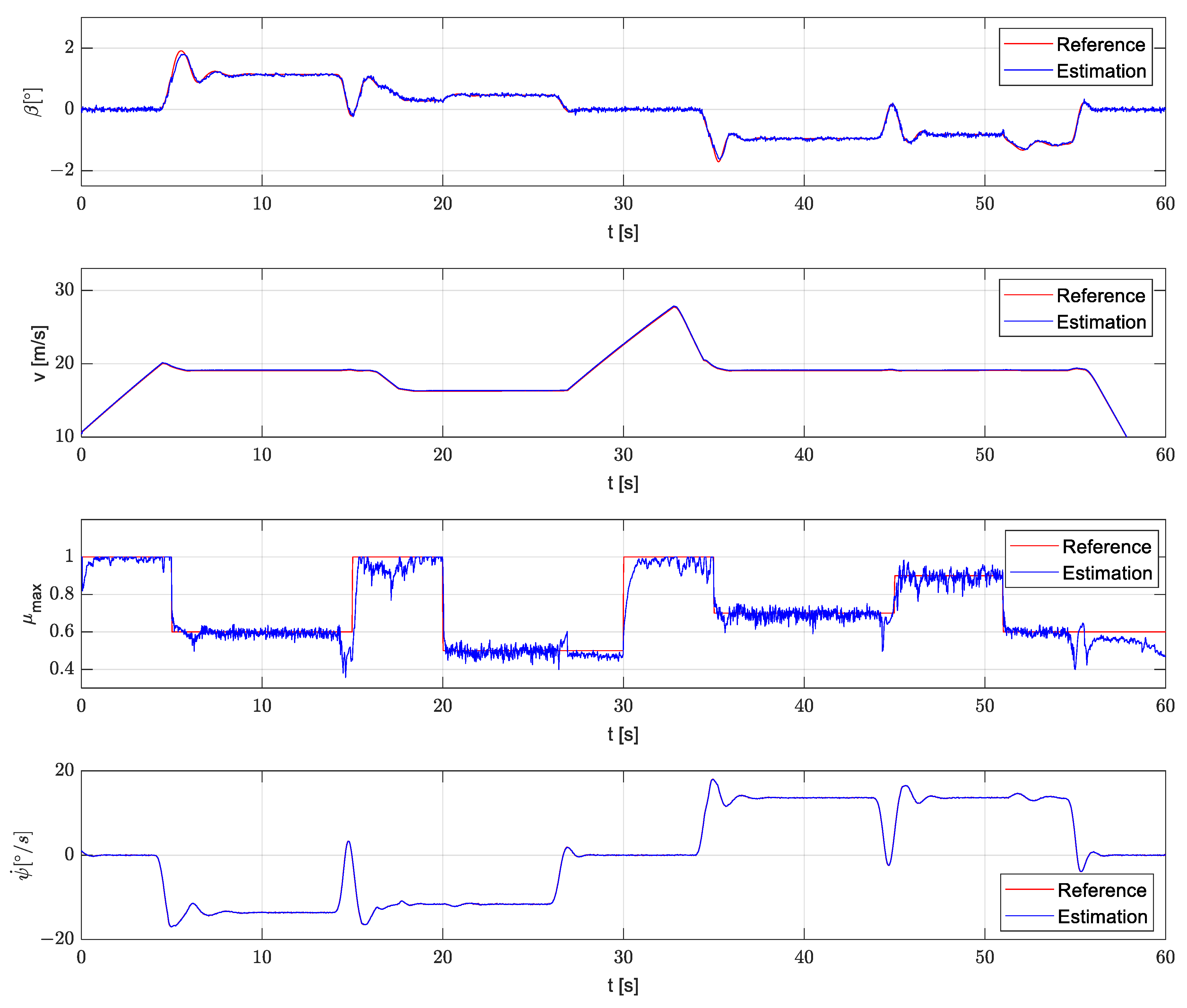
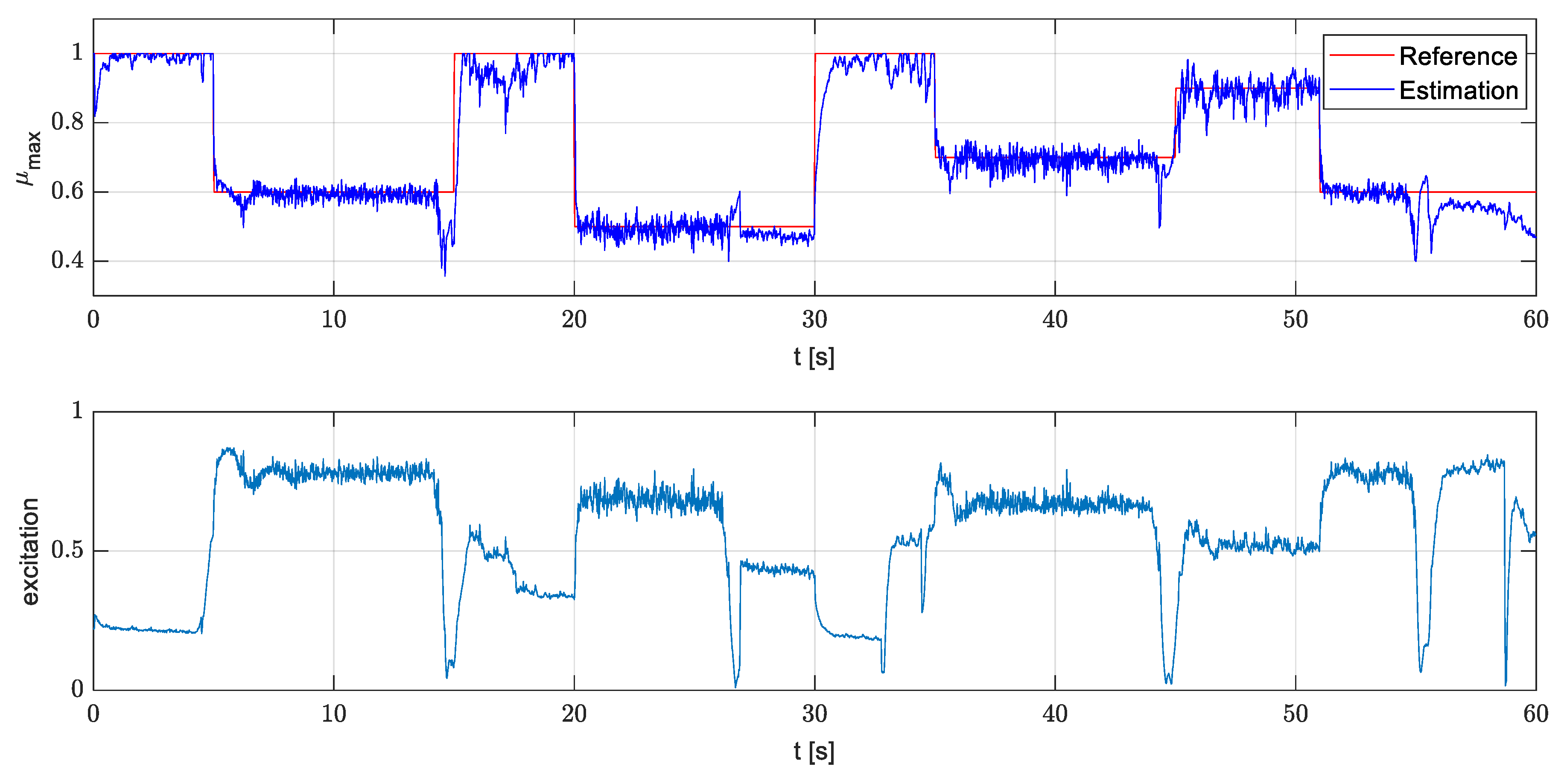
4.2. Application of the UKF-SR on a Rapid Prototyping System

The second application example deals with vehicle state estimation, focusing on the tire–road friction coefficient. Hence, a proper prediction model needs to be used for the given problem. It represents a model designed and parameterized for DLR’s ROboMObil (ROMO) [32]. This is a robotic full x-by-wire research vehicle equipped with four wheel robots. By adjusting the steering angles of the four wheels and the drive torques of the four in-wheel motors, the ROMO’s horizontal movement can be controlled. Multiple sensors are integrated into the ROMO to measure many different quantities. The vehicle model is implemented in Modelica, like the prediction model in the first scenario. It is adopted from [33], where it is described in detail.

4.2.1. Vehicle Prediction Model

The prediction model constitutes a nonlinear double-track model whose nonlinearities are primarily due to the tire model. The state vector x of the vehicle system is composed of four quantities that are estimated by means of the embedded Kalman filter library in the following. It is given by:
x = [ β       v       μ max       ψ ˙ ]
This vector includes the side-slip angle β of the vehicle, its over ground velocity v , the maximum tire-road friction coefficient μ max and the vehicle’s yaw rate ψ ˙ . The friction coefficient is a particularly interesting variable for the estimation because its direct measurement is hardly possible and its estimation is rather challenging. In particular, with regard to automated driving, the friction coefficient is an essential quantity, as it describes the road condition and, therefore, strongly influences the steering and braking dynamics of the vehicle.
The vehicle prediction model expects 11 input components:
u = [ δ fl     δ fr     δ rl     δ rr       ω fl     ω fr     ω rl     ω rr       a x , in     a y , in     ψ ˙ in ] .
This includes the respective steering angles δ i and speeds ω i of the four wheels, where the subscript i indicates the front or rear and the right or left wheels. Finally, the longitudinal and lateral acceleration a x , in and a y , in , respectively, as well as the yaw rate ψ ˙ in represent the input quantities for the Kalman filter.
The values of a x , in and a y , in are unknown inputs in the tire force equations, whose outputs are in turn the same acceleration values. Thus, this structural dependency results in an algebraic loop, see [33] (Appendix B). It is possible to obtain its solution by considering a nonlinear system of equations which is computationally expensive to solve. In addition to the limited computational capacity on embedded systems, this aspect is also problematic from a real-time capability view due to its iterative solution procedure. However, the aforementioned algebraic loop can be eliminated by including a x , in and a y , in as input variables for the prediction model, since these vehicle accelerations can be measured accurately and cost-effectively. Moreover, the yaw rate ψ ˙ in , whose accurate measurement is also possible, is taken as an additional input variable enabling open-loop evaluation of the prediction model. This is particularly advantageous in scenarios where the feedback through the measurement update (closed-loop) cannot be performed, e.g., due to measurement interruptions.
Regarding the outputs y of the prediction model, the following 10 quantities are selected and are available as measurands:
y = [ β out       v out       F y f       F y r       F x f       F x r       M z f     a x , out     a y , out     ψ ˙ out ]
This vector includes the virtual side-slip angle β out and the virtual speed v out , in addition to the virtual longitudinal ( F x f , F x r ) and lateral ( F y f , F y r ) forces of the front and rear axles, respectively. Details about these virtual measurands, which are computed by means of other measured variables, and their derivations are described in [33]. Another output of the model is the tire self-aligning torque on the front axle M z f , and, furthermore, the longitudinal and lateral accelerations a x , out and a y , out , in addition to ψ ˙ out . All of these variables are used as measured outputs in the measurement update step of the Kalman filter, see also the vector y k m in Figure 1 and Equations (A5) and (A20).

4.2.2. Integration of the Model Code in the Embedded Kalman Filter Library

In several steps the outlined Modelica prediction model of ROMO‘s vehicle dynamics is processed to suitable C code, which is finally interfaced to the model-specific functions of the embedded Kalman filter library. The process is based on the eFMI workflow [29] as described in [28] for the application example in Section 4.1. It includes the following steps:
  • the export of the Modelica model to eFMI GALEC code [29] by a Dymola prototype implementation,
  • manual modifications of the generated GALEC code to provide all necessary features and function interfaces for state estimation, and
  • the generation of eFMI production C code based on the modified GALEC code by an CATIA ESP prototype implementation. CATIA ESP is a newly developed production code generator not yet released by Dassault Systèmes.
In the first of the listed steps the prediction model equations are automatically discretized with the Explicit Euler method to ensure real-time capable code. The manual modifications in the second step are related to the eFMI function DoStep and its interface. The GALEC code is modified to enable several calls of DoStep within one sample period for different additional purposes such as repeating the integration step with different values of the states and evaluating the state derivatives and outputs for given states. These features have not yet been included in the eFMI standard proposal [29]. The generated C code of DoStep is interfaced to the library functions get_states, get_der_states and get_outputs, see Figure 2. More details on the applied process can be found in [28]. For the state estimation, the filter type UKF-SR is chosen in this application because of its higher numerical accuracy compared to the EKF-SR and a significant nonlinearity caused by the tire model.
The filter’s process and measurement noise covariance matrices Q and R , and the filter parameters α , β and κ from Table A2 are determined via an optimization approach described in [33]. They are specified using a reference trajectory obtained by means of a high-precision validated multiphysics Modelica model of the ROMO, see [33]. In contrast to the prediction model, this model represents a very detailed full vehicle model combined with an environmental model. It is utilized to generate reference data for the state estimator. The covariance matrices Q and R are determined to minimize the quadratic tracking error, i.e., the quadratic error between the estimated states and the states of the reference trajectory. The relevant system and measurement noise covariances are used as tuning parameters in this minimization problem. The optimization is carried out by applying the optimization software MOPS [34]. In the same way, the filter parameters α , β and κ are determined. For the initial guess of the state vector, which is to be set in the initialization phase of the estimation, the initial states of the reference trajectory are used.
For the estimation of the state μ max , the maximum tire friction coefficient, state constraints are introduced according to [33]. They arise from the physical limitations. The upper limit for the friction coefficient is given by the constant 1 . The lower limit, which is represented here by the currently utilized friction value, can be approximated by considering Kamm’s friction circle [33]. This limit is calculated using the longitudinal and lateral accelerations a x , in and a y , in and the gravitational acceleration g :
1 g a x , in 2 + a y , in 2 .
These constraints are implemented in the function get_state_constraints, see Section 3.2.

4.2.3. Simulation in Simulink

As the software environment surrounding the embedded Kalman filter library, a MATLAB S-function framework was chosen [35], since it can be integrated on real-time systems. Thus, simulations for validating the estimation results can be carried out in Simulink [36] by building a Simulink model that contains an S-function block. The structure of an S-function enables an easy integration of the filter algorithms, namely ukf_sr_initialize and ukf_sr_predict_correct, in the appropriate sections of the S-function. The interfaces of the S-function are adapted to provide inputs and outputs of the data type single, i.e., float, since the state estimation is also calculated with single precision. For the filter, a sample time of 20 ms is chosen, constituting a good balance between effort and precision of the state estimation.
The measured data used for y k m , see Figure 1, is synthetically generated by means of the high-fidelity Modelica model of the ROMO. Similarly, the input vector u (see (5)) and the reference data used for validating the results of the UKF-SR state estimation are also obtained by simulations of this vehicle model.
Figure 4 shows the results of the simulation of the Simulink model, which contains the UKF-SR algorithm and the prediction model code with single precision data type as an S-function and the derived inputs.
The estimated states of the model (see (4)) are depicted, as well as the reference trajectory for each state. The comparison over the entire simulation period of 60 s shows good agreement, especially for the side-slip angle β , the over ground velocity v and the yaw rate ψ ˙ . The maximum friction coefficient μ max can also follow its reference trajectory well. Corresponding to the introduced state constraints, the friction coefficient does not exceed the upper limit of 1 . However, slight deviations of the estimation occur, e.g., at 15 s, 44 s and 55 s. An explanation for this relates to the excitation of the system as follows.
The prescribed driving path of the reference vehicle to generate the input data u represents a crossing eight; see [33]. Different lateral and longitudinal excitations occur in the process, due to braking, accelerating and steering. The overall excitation results from the consideration of Kamm’s friction circle and is given by the following formula [33]:
1 g μ max a x , in 2 + a y , in 2 .
It utilizes the lateral and longitudinal accelerations of the vehicle a y , in and a x , in , respectively, and the gravitational acceleration g . Figure 5 shows the time dependent plot of this excitation and of the friction coefficient from Figure 4 for convenient comparison.
The parts of the simulation range, where the friction coefficient shows the outliers, correspond to phases with a low input excitation. In [33] it is demonstrated that, in these passages the observability of the dynamical system decreases since the excitation is below a necessary threshold. For the friction coefficient, this leads to episodes where the estimation drifts away from the reference.

4.2.4. Execution on the Rapid Prototyping Platform

After this successful validation of the UKF-SR filter in a simulation, the algorithm is further employed on a dSPACE MicroAutoBox II (MABX) [37]. This represents a real-time system enabling fast function prototyping. The applied Simulink model contains, again, the UKF-SR algorithm with the prediction model code in 32-bit precision as an S-function. The inputs u and y k m for the state estimation, which were already used for the simulation in Figure 4, are included as time dependent data points in the model. The Simulink model is processed by means of Real-Time Interface [38]. This software provides an interface between the MABX and Simulink and generates code for the model. After the successful completion of the build procedure for the Simulink model comprising the filter, the generated files are loaded into ControlDesk [39], which runs the application on the real-time system and performs the measurement and logging of the signals.
The UKF-SR estimator was successfully run in real-time. The time needed to execute one task on the MABX resides at a maximum of 1.3 ms which is significantly lower than the sample time of the filter, which is 20 ms. The evaluation of the recorded signals on the platform shows a high agreement with the corresponding results of the offline Simulink simulation in Figure 4. The maximum absolute differences between these two estimations are in the range of 10 3 to 10 6 , depending on the considered state. They are thus in the expected range when comparing two single precision signals. In total, the good results of the state estimation from the offline Simulink simulation are reproduced on the embedded platform in real-time.
The application employed here represents a desktop setup with the MABX and a laptop. However, the state estimator could also be used in the equivalent configuration in a MABX installed in a vehicle. In this scenario, the inputs for the estimation would be provided directly by the measurements of the real sensors and the results of the estimation could be processed in real driving operation.

5. Conclusions

In this paper, a new embedded Kalman filter library is introduced. It was implemented in C with the goal of performing state estimation on embedded systems, for example, in the context of designing controllers for vehicle system dynamics. The library contains different variants of nonlinear Kalman filters: the EKF-SR and the UKF-SR. The UKF-SR provides the advantage of higher accuracy compared to the EKF-SR, whereas the EKF-SR allows for a shorter execution time. The square-rooting (SR) variants increase the numerical stability and provide a greater robustness compared to the base filters. During implementation, an emphasis was placed on ensuring that the code complies widely with the requirements for safety-critical applications in the automotive sector. The commonly used programming language C is suitable for this purpose and was, therefore, chosen for the new library. It also enables an easy integration into tool chains for embedded systems. The MISRA C coding guidelines were also considered during the implementation. Numerical computations required for the state estimation algorithms are partially based on existing and well-established functions such as LAPACK routines, as they have already proven their efficiency. All of these are newly implemented in C, yielding self-contained software without the need for external libraries.
For execution on embedded systems, the real-time capability of the software is another important factor, in addition to running in a 32-bit single precision configuration. The library proved its real-time capability in two application examples for vehicle state estimation. The two Kalman filter variants, the EKF-SR and the UKF-SR, were tested in two different scenarios. The vehicle models used in the respective cases comprise a nonlinear quarter vehicle model and a nonlinear double-track model. In both cases, the code for the model representations was generated through a modified eFMI export and then interfaced to the model-specific functions of the library. The filter algorithms were integrated in two different embedded systems. Code generation for the respective platforms was carried out by means of TargetLink and Real-Time Interface. The underlying C code of the Kalman filter library was incorporated into the executed production code as custom code.
The two scenarios were aimed at different purposes. First, it was shown that the state estimator was able to provide reasonably good results under challenging real-time conditions in a small-scale production series ECU within a vehicle in real-world driving tests. In the second application, special emphasis was placed on the accuracy of the filter, which was able to follow well the synthetically generated reference data on a rapid prototyping platform. In both examples, the embedded Kalman filter library was successfully implemented on an embedded system using appropriate tool chains and it achieved good results under real-time constraints.
The embedded Kalman filter library will be used in future internal research projects. For common research projects with interested readers, the authors may be contacted.

Author Contributions

Conceptualization, C.S., A.P. and J.B.; methodology, C.S., A.P. and J.R.; library software, C.S.; application software and data, C.S., A.P. and J.R.; validation, C.S., A.P. and J.R.; formal analysis, C.S. and A.P.; investigation, C.S., A.P. and J.R.; visualization, C.S.; writing—original draft preparation, C.S.; writing—review and editing, C.S., A.P., J.R. and J.B.; supervision, J.B. and A.P. All authors have read and agreed to the published version of the manuscript.

Funding

This work was mainly funded by DLR internal projects. Parts of the work were funded by the German Federal Ministry of Education and Research (grant number 01|S17023B) within the European ITEA3 project EMPHYSIS (Embedded systems with physical models in the production code software) under the project number 15016.

Data Availability Statement

Not applicable.

Acknowledgments

The authors’ thanks go to Dassault Systèmes for providing prototypical tools for eFMI export and to Daniel Baumgartner for his support with the real-time tests.

Conflicts of Interest

The authors declare no conflict of interest.

Appendix A. Kalman Filter Algorithms

In this appendix, the basic theory of four nonlinear Kalman filter based state estimation algorithms is described: the EKF, EKF-SR, UKF and UKF-SR. Detailed information about this subject can be found in [1,18,19]. The following overview is based on [20], particularly with regard to formulas and notations.

Appendix A.1. Extended Kalman Filter (EKF)

The EKF is able to handle models including nonlinearities by linearizing the model around the last estimation point. Therefore, a Taylor series evaluation is carried out, which can be implemented numerically by means of a forward difference quotient. The steps of the EKF algorithm are shown in Table A1 as a pseudo code, see [20].
Table A1. Pseudo code of the EKF algorithm.
Initialization:
x ^ 0 + = E ( x 0 )
P 0 + = E ( ( x 0 x ^ 0 + ) ( x 0 x ^ 0 + ) T )
(A1)
For   k = 1 , 2 ,
Predict:
x ^ k = f k | k 1 ( x ^ k 1 + , u k 1 ) (A2)
P k = F k 1 P k 1 + F k 1 T + Q with F k 1 = e ( J k 1 T s ) = e ( f x | x ^ k 1 + T s ) (A3)
Correct:
K k = P k H k T ( H k P k H k T + R ) 1 with H k = h x | x ^ k (A4)
x ^ k + = x ^ k + K k ( y k m h ( x ^ k ) ) (A5)
P k + = ( I K k H k ) P k (A6)
The operator E ( ) in the initialization phase determines the expectation value of the specified variables [20]. T s represents the sample time and K k the Kalman gain. The covariance matrices Q and R are defined by the user and they can be employed to adjust the filter to the respective application. The matrix Q denotes the process noise covariance. It evaluates the trust in the a priori estimation. The measurement noise covariance R reflects the confidence in the measurements y k m . The matrix F k 1 is the state transition matrix of the function f with respect to x at the point x ^ k 1 + . It is computed by means of a matrix exponential function evaluating the system state Jacobian J k 1 . The latter can be calculated numerically, if it is not available in analytical form. This can be carried out using a forward difference quotient as follows:
For   i = 1 , 2 , , n x : ( J k 1 ) i = f ( x ^ k 1 + Δ e i , u k 1 ) f ( x ^ k 1 , u k 1 ) Δ with   Δ ϵ
In this formula, n x denotes the number of states of the system and e i is the i -th unit vector. The radicand ϵ represents the respective machine precision of the employed computer system. The output Jacobian matrix H k of the function h with respect to x at the point x ^ k is computed analogous to the Jacobian J k 1 with a forward difference quotient as in (A7). Performing the steps in Table A1, the new estimated states vector x ^ k + is computed using the results from the last sample time step and the current output measurement vector y k m . In Table A1, the model evaluation of the underlying system equations is necessary for computing the Jacobians J k 1 and H k , h , and f k | k 1 , whereas the latter denotes the integration from the last sample point to the new one; see Equation (3).

Appendix A.2. Extended Kalman Filter with Square-Rooting (EKF-SR)

The approach of the EKF implementation described in Section A.1 may possibly lead to numerical difficulties, as briefly outlined in [1]. In particular, the use on embedded systems with limited memory and computing resources is sensitive in this respect. For example, the computation of the matrix P k + as a difference of two matrices in (A6) may result in a matrix that is not positive definite in case of insufficient accuracies. This constitutes a problem because the matrix P k + is a covariance matrix and is therefore required to be positive definite. These numerical difficulties can be handled by using the square-root form of a matrix. This can be implemented by a Cholesky factorization:
P k + = L k L k T
Thereby, a symmetric and positive definite matrix P k + is decomposed into a product of a lower triangular matrix L k and its transpose. Instead of the original matrix, the decompositions are used in the algorithm. This approach provides a higher numerical stability and the positive definiteness of the covariance matrix is easier to maintain. Furthermore, as shown in [20], the square-root of a matrix has a condition number that is the square-root of the condition number of the original matrix, which helps to improve the numerical accuracy of the algorithm.

Appendix A.3. Unscented Kalman Filter (UKF)

Another observer design that can handle state estimation with nonlinearities in the model is the unscented Kalman filter (UKF). The name is derived from the unscented transformation of disturbed state vectors. It represents a way of obtaining the statistics, i.e., the mean and covariance, of a random variable that is subject to a nonlinear transformation [40]. In comparison to the EKF, the nonlinear approximation is at least twice as accurate, and therefore the UKF is better suited for models with strong nonlinearities [40]. Furthermore, it is not necessary to calculate the state and output Jacobian matrices of the nonlinear prediction model in the UKF. The basic idea of this filter variant is briefly described below, based on [19,20,40], which can also be referred to for further details.
The use of the unscented transformation is carried out because of the assessment that a Gaussian distribution is easier to approximate than another arbitrary nonlinear transformation [20]. As in the EKF, a Gaussian random variable is used to display the state distribution. The new aspect in the UKF is its representation by a minimum setup of properly selected sample points. These are the so-called sigma points. They are selected around the current estimation point and are chosen in a heuristic way. The sigma points are propagated through the nonlinear function of the underlying prediction model, with no approximation performed [19]. In this way, the estimated mean and covariance is obtained with an accuracy of the third order of a Taylor series expansion for Gaussian inputs. For non-Gaussian distributions the achieved accuracy of the approximation is of the second order [19]. This is the reason for the beforementioned higher approximation accuracy of the UKF in comparison to the EKF, where the linearization approach leads to an accuracy of the first order.
An important component within the UKF algorithm is the evaluation of the sigma points. Their selection is carried out by means of a static scaling parameter and the covariance matrix P + , which was calculated in the a posteriori step, see Figure 1. A total of 2 n x + 1 sigma vectors is obtained. The resulting vectors are used as disturbed state inputs for 2 n x + 1 integrations of the nonlinear system, which are performed from the last sample point t k 1 to the new one t k . Some parameters are necessary for the calculation of the sigma points and their corresponding weightings. They must be set at the beginning of the algorithm and can be tuned for the respective application. A summary of these parameters is shown in Table A2, see also [20].
Table A2. Parameters of the UKF.
ParameterDescription
α Spread of the sigma points around the current mean x ^
β Characteristic of the stochastic distribution
κ Scaling kurtosis of the sigma points
For the utilized approach of the unscented transformation a matrix X n x × ( 2 n x + 1 ) is created. It is composed of the 2 n x + 1 sigma vectors representing the columns of the matrix. These sigma vectors are calculated using the current mean x ^ and the covariance matrix P + . The formulas for the calculation of the vectors is shown in Table A3. It is related to [40].
Table A3. Sigma vectors with scaling parameter γ .
γ = α n x + κ
X 1 = x ^
X i = x ^ + ( γ P + ) i 1 ,         i = 2 , , n x + 1
X i = x ^ ( γ P + ) i 1 n x ,         i = n x + 2 , , 2 n x + 1
The expression P + in these equations determines the matrix square-root of the covariance matrix. Table A3 also specifies the scaling parameter γ , which depends only on the parameters of Table A2 and the dimension of the system states. The term ( γ P + ) i denotes the i th column of the corresponding matrix.
The resulting sigma points are assigned with weights in the UKF algorithm. These scalar weightings are summarized in Table A4, see also [20]. They depend on the parameters in Table A2.
Table A4. Set of weights in the UKF.
WeightDescription
λ = α 2 ( n x + κ ) n x Scaling parameter
a = α 2 ( n x + κ ) Scaling parameter
w 0 m = λ a Weight of unmodified mean prediction
w 0 c = λ a + 1 α 2 + β Weight of unmodified output mean prediction
w i m = w i c = 1 2 a ,   i = 1 , , 2 n x Weight of sigma points of states and outputs
With these prerequisites, the steps of the UKF algorithm can now be outlined. The general structure of the UKF resembles the corresponding EKF algorithm setup in Table A1. Its scheme is again composed of a predict and a correct step after an initialization, like in Figure 1. The algorithm of the UKF is given as pseudo code in Table A5 and is based on [20].
Table A5. Pseudo code of the UKF algorithm.
Initialization:
x ^ 0 + = E ( x 0 )
P 0 + = E ( ( x 0 x ^ 0 + ) ( x 0 x ^ 0 + ) T )
(A9)
For   k = 1 , 2 ,
Predict:
X k 1 = [ x ^ k 1 + ,       X ^ k 1 + + γ P k 1 + ,             X ^ k 1 + γ P k 1 + ] (A10)
X k | k 1 = f k | k 1 ( X k 1 , u k 1 ) (A11)
x ^ k = i = 0 2 n x w i m ( X k | k 1 ) i + 1 (A12)
P k = i = 0 2 n x w i c [ ( X k | k 1 ) i + 1 x ^ k ] [ ( X k | k 1 ) i + 1 x ^ k ] T + Q (A13)
X k = [ x ^ k ,       X ^ k + γ P k ,             X ^ k γ P k ] (A14)
Y k = h ( X k ) (A15)
y ^ k = i = 0 2 n x w i m ( Y k ) i + 1 (A16)
Correct:
P y k = i = 0 2 n x w i c [ ( Y k ) i + 1 y ^ k ] [ ( Y k ) i + 1 y ^ k ] T + R (A17)
P x k y k = i = 0 2 n x w i c [ ( X k | k 1 ) i + 1 x ^ k ] [ ( Y k ) i + 1 y ^ k ] T (A18)
K k = P x k y k P y k 1 (A19)
x ^ k + = x ^ k + K k ( y k m y ^ k ) (A20)
P k + = P k K k P y k K k T (A21)
In the above notations, there are some expressions of a function with a matrix instead of a vector as an argument, for example h ( X k ) in (A15). This term corresponds to evaluating each column of the matrix separately and returning this as a result, again in a matrix representation. It is defined X ^ k 1 + : = [ x ^ k 1 + , x ^ k 1 + , , x ^ k 1 + ] n x × n x in (A10) and X ^ k : = [ x ^ k , x ^ k , , x ^ k ] n x × n x in (A14). The matrix square-roots of the covariance matrices are calculated by means of Cholesky factorizations. The time and measurement update equations comprise more calculations in the UKF, compared to the EKF, including the evaluation of the sigma points. The concatenated matrix X k 1 provides the sigma vectors from Table A3. The following step in the pseudo code in (A11) represents the integration performed 2 n x + 1 times between the last sample point t k 1 and the new one t k . For this purpose, for example, an Euler method can be applied and the sigma points serve as disturbed state inputs for the integration. The set of scalars as determined in Table A4, is employed in the calculations of x ^ k , y ^ k and P k in the predict step, where weighted sums are used. The matrices Q and R define again, as in the EKF, the respective covariances for process and measurement noises. By tuning them, the trust in the measurements can be stated.

Appendix A.4. Unscented Kalman Filter with Square-Rooting (UKF-SR)

As it is the case with the EKF, a square-rooting approach also applies to the UKF, which is accordingly called UKF-SR. The principle algorithm equations are maintained compared to the UKF, and also the parameters, sigma points and weights as described in Table A2, Table A3 and Table A4 remain the same. A new aspect of this filter variant is the exploitation of the structure of the covariances. As shown in Table A5, in the UKF the full covariance P k + is recursively updated in each step, although the square-root of this matrix is an essential part of the algorithm [19]. As such, only the Cholesky factors P k 1 + and P k , respectively, are used to determine the sigma points, and the entire covariance matrix is not required in these calculations. Another step where the use of Cholesky factors is valuable is the evaluation of the Kalman gain matrix K k . In the UKF, this is performed in (A19) by solving a linear system of equations K k = P x k y k P y k 1 . With the means of Cholesky factors, this step can be performed more efficiently. Moreover, since the covariance matrix is uniquely determined by its Cholesky factors, it is not necessary to perform its explicit computation at each step.
As in the UKF, in the UKF-SR algorithm a Cholesky factorization is also carried out at the beginning to calculate the square-root of the state covariance matrix. Since this matrix is symmetric and positive definite, a Cholesky decomposition is always feasible. The factorization is performed into a lower and upper triangular matrix; see (A8). In the following steps, only the lower triangular matrix is considered. In contrast to the UKF, with the UKF-SR only this Cholesky decomposition is propagated directly and updated in the following iterations of the algorithm. Therefore, rank one updates or downdates of the Cholesky factor matrix are deployed. By using these, modifications are applied directly to the Cholesky factor and there is no need to perform a new matrix decomposition. The calculation of the matrix P k in (A13) in the predict step of the UKF in Table A5 is now replaced by the following two operations, see [20]:
C P k = LQ ( [ w 1 c ( ( X k | k 1 ) i x ^ k ) i = 2 : 2 n x + 1 , Q ] ) C P k : = cholupdate ( C P k , ( X k | k 1 ) 1 x ^ k , w 0 c )
The expression C P k denotes the Cholesky factor of the covariance matrix P k . In the first step of (A22) a LQ factorization is carried out. The operand is a composed matrix including the weighted propagated sigma vectors and the square-root of the process noise covariance matrix Q . The LQ factorization partitions the resulting matrix into a lower triangular matrix with positive diagonal elements and an orthogonal matrix. Only the first is computed directly and returned by the function LQ. The LQ factorization replaces an equivalent QR decomposition. It is used to achieve consistency with other operations where the lower triangular part of a matrix is incorporated [20]. In the next step of (A22), a rank one update of the Cholesky factor is performed. It is assumed P = C P C P T . The notation cholupdate ( C P , v , ± 1 ) calculates a lower triangular matrix C P * = C P ± v v T where the positive definiteness of the matrix P * = C P * C P * T is guaranteed [20]. More details about rank updates for Cholesky decompositions can be found in [24,27]. The second step in (A22) is required because the weight w 0 c could be negative. These two operations in (A22) perform the time update of the Cholesky factor; see also [19].
The same approach is utilized in the calculation of the Cholesky factor of the observation error covariance. The calculation of the matrix P y k in (A17) in the correct step of the UKF in Table A5 is thus replaced by the following two steps:
C P y k = LQ ( [ w 1 c ( ( Y k ) i y ^ k ) i = 2 : 2 n x + 1 , R ] ) C P y k : = cholupdate ( C P y k , ( Y k ) 1 y ^ k , w 0 c )
These operations are similar to the corresponding steps in (A22). The evaluation of the Kalman gain matrix K k in (A19) is performed by the equation:
K k = P x k y k ( C P y k T C P y k ) 1
This can be solved efficiently using backward substitutions. The last adaptation of the UKF algorithm concerns the last item of Table A5 where the measurement update of the state covariance P k + is calculated in (A21). It is replaced by these operations:
U = K k C P y k C P k + = cholupdate ( C P k , U , 1 )
To the former computed Cholesky factor C P k , several consecutive Cholesky rank one downdates are applied, see [19]. They are executed using the n y columns of the matrix U , where n y denotes the dimension of the outputs of the system equations.
With these modifications of the UKF algorithm, the UKF-SR algorithm is adequately described. The refactorization of the covariance matrices in each step can be omitted because the decomposed Cholesky factors are propagated directly. Hence, the state covariance matrices acquire the ensured property of positive semi-definiteness [19]. This advantage promotes the improvement in numerical properties of the UKF-SR algorithm and provides greater robustness to numerical instabilities in comparison to the UKF [20].

References

  1. Haykin, S. Kalman Filtering and Neural Networks; John Wiley & Sons, Inc.: New York, NY, USA, 2001. [Google Scholar]
  2. Karamta, M.R.; Jamnani, J.G. Implementation of extended kalman filter based dynamic state estimation on SMIB system incorporating UPFC dynamics. Energy Procedia 2016, 100, 315–324. [Google Scholar] [CrossRef] [Green Version]
  3. Li, J.-M.; Chen, C.W.; Cheng, T.-H. Estimation and Tracking of a Moving Target by Unmanned Aerial Vehicles. In Proceedings of the American Control Conference (ACC), Philadelphia, PA, USA, 10–12 July 2019. [Google Scholar]
  4. Wutke, M.; Heinrich, F.; Das, P.P.; Lange, A.; Gentz, M.; Traulsen, I.; Warns, F.K.; Schmitt, A.O.; Gültas, M. Detecting animal contacts—A deep learning-based pig detection and tracking approach for the quantification of social contacts. Sensors 2021, 21, 7512. [Google Scholar] [CrossRef] [PubMed]
  5. Al Khatib, E.I.; Jaradat, M.A.; Abdel-Hafez, M.; Roigari, M. Multiple Sensor Fusion for Mobile Robot Localization and Navigation Using the Extended Kalman Filter. In Proceedings of the 10th International Symposium on Mechatronics and Its Applications (ISMA), Sharjah, United Arab Emirates, 8–10 December 2015. [Google Scholar]
  6. Ullah, I.; Su, X.; Zhang, X.; Choi, D. Simultaneous localization and mapping based on Kalman filter and extended Kalman filter. Wirel. Commun. Mob. Comput. 2020, 2020, 2138643. [Google Scholar] [CrossRef]
  7. Fossen, S.; Fossen, T.I. Five-state extended Kalman filter for estimation of Speed over Ground (SOG), Course over Ground (COG) and Course Rate of Unmanned Surface Vehicles (USVs): Experimental results. Sensors 2021, 21, 7910. [Google Scholar] [CrossRef] [PubMed]
  8. Vergori, E.; Mocera, F.; Somà, A. Battery modelling and simulation using a programmable testing equipment. Computers 2018, 7, 20. [Google Scholar] [CrossRef] [Green Version]
  9. Colonnier, F.; della Vedova, L.; Orchard, G. ESPEE: Event-based sensor pose estimation using an extended Kalman filter. Sensors 2021, 21, 7840. [Google Scholar] [CrossRef] [PubMed]
  10. Ponte, S.; Ariante, G.; Papa, U.; del Core, G. An embedded platform for positioning and obstacle detection for small unmanned aerial vehicles. Electronics 2020, 9, 1175. [Google Scholar] [CrossRef]
  11. Fico, V.M.; Arribas, C.P.; Soaje, Á.R.; Prats, M.Á.M.; Utrera, S.R.; Vázquez, A.L.R.; Casquet, L.M.P. Implementing the Unscented Kalman Filter on an Embedded System: A Lesson Learnt. In Proceedings of the IEEE International Conference on Industrial Technology (ICIT), Seville, Spain, 17–19 March 2015. [Google Scholar]
  12. EEKF—Embedded Extended Kalman Filter. 2015. Available online: https://github.com/dr-duplo/eekf (accessed on 4 October 2022).
  13. Valade, A.; Acco, P.; Grabolosa, P.; Fourniols, J.-Y. A study about Kalman filters applied to embedded sensors. Sensors 2017, 17, 2810. [Google Scholar] [CrossRef] [PubMed] [Green Version]
  14. Rasmussen, T.B.; Yang, G.; Nielsen, A.H.; Dong, Z.Y. Implementation of a Simplified State Estimator for Wind Turbine Monitoring on an Embedded System. In Proceedings of the 2017 Federated Conference on Computer Science and Information Systems, Prague, Czech Republic, 3–6 September 2017; pp. 1167–1175. [Google Scholar]
  15. Motor Industry Software Reliability Association. MISRA-C:2012. 2012. Available online: https://www.misra.org.uk/ (accessed on 4 October 2022).
  16. Bagnara, R.; Bagnara, A.; Hill, P.M. The MISRA C Coding Standard and Its Role in the Development and Analysis of Safety- and Security-Critical Embedded Software. In Proceedings of the Static Analysis: The 25th International Symposium (SAS 2018), Freiburg, Germany, 29–31 August 2018. [Google Scholar]
  17. Anderson, E.; Bai, Z.; Bischof, C.; Blackford, L.S.; Demmel, J.; Dongarra, J.; Croz, J.D.; Greenbaum, A.; Hammarling, S.; McKenney, A.; et al. LAPACK Users’ Guide, 3rd ed.; Society for Industrial and Applied Mathematics: Philadelphia, PA, USA, 1999. [Google Scholar]
  18. Simon, D. Optimal State Estimation: Kalman, H Infinity, and Nonlinear Approaches; John Wiley & Sons, Inc.: Cleveland, OH, USA, 2006. [Google Scholar]
  19. van der Merwe, R.; Wan, E.A. The Square-Root Unscented Kalman Filter for State and Parameter-Estimation. In Proceedings of the IEEE International Conference on Acoustics, Speech, and Signal Processing, Salt Lake City, UT, USA, 7–11 May 2001. [Google Scholar]
  20. Brembeck, J. Model Based Energy Management and State Estimation for the Robotic Electric Vehicle ROboMObil. Ph.D. Thesis, Technische Universität München, Munich, Germany, 2018. [Google Scholar]
  21. Kandepu, R.; Imsland, L.; Foss, B.A. Constrained State Estimation Using the Unscented Kalman Filter. In Proceedings of the 16th Mediterranean Conference on Control and Automation, Ajaccio, France, 25–27 June 2008; pp. 1453–1458. [Google Scholar]
  22. Brembeck, J. A physical model-based observer framework for nonlinear constrained state estimation applied to battery state estimation. Sensors 2019, 19, 4402. [Google Scholar] [CrossRef] [PubMed] [Green Version]
  23. Brembeck, J. Nonlinear constrained moving horizon estimation applied to vehicle position estimation. Sensors 2019, 19, 2276. [Google Scholar] [CrossRef] [PubMed]
  24. Golub, G.H.; Van Loan, C.F. Matrix Computations, 4th ed.; The Johns Hopkins University Press: Baltimore, MA, USA, 2013. [Google Scholar]
  25. Modelica Association. Modelica Standard Library v4.0.0. 2020. Available online: https://github.com/modelica/ModelicaStandardLibrary/releases/tag/v4.0.0 (accessed on 21 September 2022).
  26. Netlib. LAPACK Documentation. 2022. Available online: http://www.netlib.org/lapack/explore-html/ (accessed on 4 October 2022).
  27. Seeger, M. Low Rank Updates for the Cholesky Decomposition; Department of EECS, University of California at Berkeley: Berkeley, CA, USA, 2008. [Google Scholar]
  28. Ultsch, J.; Ruggaber, J.; Pfeiffer, A.; Schreppel, C.; Tobolář, J.; Brembeck, J.; Baumgartner, D. Advanced controller development based on eFMI with applications to automotive vertical dynamics control. Actuators 2021, 10, 301. [Google Scholar] [CrossRef]
  29. Lenord, O.; Otter, M.; Bürger, C.; Hussmann, M.; le Bihan, P.; Niere, J.; Pfeiffer, A.; Reicherdt, R.; Werther, K. eFMI: An Open Standard for Physical Models in Embedded Software. In Proceedings of the 14th International Modelica Conference, Linköping, Sweden, 20–24 September 2021. [Google Scholar]
  30. Modelica Association. Modelica Language Specification 3.5. 2021. Available online: https://modelica.org/documents/MLS.pdf (accessed on 23 September 2022).
  31. dSPACE GmbH. TargetLink. 2022. Available online: https://www.dspace.com/en/pub/home/products/sw/pcgs/targetlink.cfm (accessed on 6 September 2022).
  32. Brembeck, J.; Ho, L.M.; Schaub, A.; Satzger, C.; Tobolar, J.; Bals, J.; Hirzinger, G. ROMO—The Robotic Electric Vehicle. In Proceedings of the 22nd IAVSD International Symposium on Dynamics of Vehicle on Roads and Tracks, Manchester, UK, 11–14 August 2011. [Google Scholar]
  33. Ruggaber, J.; Brembeck, J. A novel Kalman filter design and analysis method considering observability and dominance properties of measurands applied to vehicle state estimation. Sensors 2021, 21, 4750. [Google Scholar] [CrossRef] [PubMed]
  34. Joos, H.-D.; Bals, J.; Looye, G.; Schnepper, K.; Varga, A. A Multi-Objective Optimisation-Based Software Environment for Control Systems Design. In Proceedings of the IEEE International Conference on Control Applications and International Symposium on Computer Aided Control Systems Design, Glasgow, UK, 18–20 September 2002. [Google Scholar]
  35. The MathWorks, Inc. Write Level-2 MATLAB S-Functions. 2022. Available online: https://de.mathworks.com/help/simulink/sfg/writing-level-2-matlab-s-functions.html (accessed on 4 October 2022).
  36. The MathWorks, Inc. Simulink. 2022. Available online: https://www.mathworks.com/products/simulink.html?s_tid=hp_ff_p_simulink (accessed on 6 September 2022).
  37. dSPACE GmbH. MicroAutoBox II. 2022. Available online: https://www.dspace.com/en/inc/home/products/hw/micautob/microautobox2.cfm (accessed on 4 October 2022).
  38. dSPACE GmbH. Real-Time Interface (RTI). 2022. Available online: https://www.dspace.com/en/inc/home/products/sw/impsw/real-time-interface.cfm (accessed on 6 September 2022).
  39. dSPACE GmbH. ControlDesk. 2022. Available online: https://www.dspace.com/en/pub/home/products/sw/experimentandvisualization/controldesk.cfm (accessed on 6 September 2022).
  40. Wan, E.A.; van der Merwe, R. The Unscented Kalman Filter for Nonlinear Estimation. In Proceedings of the IEEE Symposium on Adaptive Systems for Signal Processing, Communications, and Control, Lake Louise, AB, Canada, 4 October 2000. [Google Scholar]
Figure 1. Scheme of state estimation using Kalman filtering.
Computers 11 00165 g001
Figure 2. Diagram of the general structure of the embedded Kalman filter library.
Computers 11 00165 g002
Figure 3. Interfaces of the function xkf_sr_predict_correct to the surrounding software environment.
Computers 11 00165 g003
Figure 4. Results of the UKF-SR state estimation in Simulink, depicting the estimated states of (4) as well as reference trajectories from the simulation of the high-fidelity Modelica vehicle model.
Computers 11 00165 g004
Figure 5. Estimated and reference friction coefficient from Figure 4, compared to the excitation of the system from (8).
Computers 11 00165 g005
Table 1. Code segment to define the data type and macros depending on the chosen precision.
#define single_precision
#ifdef double_precision
  typedef double real_t;
  #define ukf_sr_fabs fabs
  #define ONE 1.0
#elif defined single_precision
  typedef float real_t;
  #define ukf_sr_fabs fabsf
  #define ONE 1.0f
#endif
Publisher’s Note: MDPI stays neutral with regard to jurisdictional claims in published maps and institutional affiliations.

