Article

Solution of Extended Multi-Objective Portfolio Selection Problem in Uncertain Environment Using Weighted Tchebycheff Method

Division of Mathematics, School of Advanced Science and Languages, VIT Bhopal University, Sehore 466114, India
Computers 2022, 11(10), 144; https://doi.org/10.3390/computers11100144
Submission received: 22 August 2022 / Revised: 14 September 2022 / Accepted: 19 September 2022 / Published: 22 September 2022

Abstract

:
In this paper, a mathematical model for an extended multi-objective portfolio selection (EMOPS) problem is explored with liquidity considered as another objective function besides the risk and return. The model is mathematically formulated in an uncertain environment. The concerned uncertainty is dealt with by employing the fuzzy numbers in the risk matrix and return. While the fuzzy EMOPS model is converted into the corresponding deterministic case based on the α level sets of the fuzzy numbers, a weighted Tchebycheff method is implemented by defining relative weights and ideal targets. The merit of the suggested method is the applicability in many real-world situations. At the end, some numerical illustration is exhibited for the utility of the suggested EMOPS problem. Finally, it is concluded that the suggested method is simple to learn and to implement in real-life situations for the decision maker.

1. Introduction

The problems concerning portfolio selection (PS) are referred to with the formation of portfolio satisfaction. The availability of uncertainty on the securities’ returns makes it difficult to ensure which portfolio should be chosen (Simammora and Sashanti [1]).
In numerous application-related areas, for instance, system analytics and optimization, an optimization model is formulated by employing the data that is disclosed with some approximation. Fuzzy sets theory, as invented by Zadeh [2] helps to deal with the possible uncertainty in the model using the fuzzy numbers. Dubois and Prade [3] studied the fuzzification rule to deal with the mathematical operations in the domain of real numbers to the co-domain of fuzzy numbers. Rommelfonger et al. [4] presented an efficient methodology to solve the multi-objective linear programming (MOLP) problem. Zhao et al. [5] determined the solution for the most generalized symmetrical fuzzy LP problem, where both fuzzy (non-fuzzy) equality and inequality constraints are included. Fuzzy LP with multiple objective functions was introduced by Zimmermann [6]. The neutrosophic sets, which are the generalized forms of fuzzy sets, are employed to solve the fuzzy multi-objective linear programming model (Ahmadini and Ahmad, [7]).
Due to the uncertainty available in the parameters of real-world application models, the actual return of each security is not prespecified well in advance. The theory of optimal portfolios has been developed by Markowitz [8], where he has firstly studied the mean-variance model. The PS problem is typically an LP model when the return of each security is constant. Tanaka et al. [9] extended the probability into a fuzzy probability for the Markowitz’s model. Hassuike et al. [10] proposed several models for PS problems, particularly a scenario model including ambiguous factors. Ammar and Khalifa [11] developed a fuzzy PS problem using an LP approach. Khalifa and Zein [12] proposed a PS problem assuming the fuzzy objective function coefficients and implemented the fuzzy approach to determine the α optimal compromise solutions. Luengo [13] studied the PS problem under the fuzzy environment. Bermudez et al. [14] developed the PS problem with three objective functions to find tradeoffs between risk, return, and the number of securities in the portfolio. Xu and Li [15] introduced a class of stochastic multi-objective problems considering a quadratic, various types of linear objectives with linear constraints and its application on the PS model.
Chalco et al. [16] suggested a two-parameter representation for interval number representations, for instance, decreasing/increasing convex constraint functions. Fard and Ramezanzadeh [17] investigated the constrained fuzzy-valued optimization problems. Glensk and Madlener [18] introduced different types of PS models with the return rates as well as the investors’ aspiration levels of portfolio return and risk as fuzzy numbers. Moghadam et al. [19] studied a two-stage model, which in the first stage computes the required per cent of investment in every industrial group utilizing the return as well as the risk measure. Panwar et al. [20] introduced a hybrid methodology for the allocation of asset, providing a combination of many methodologies to facilitate ranking the assets. Qian and Yin [21] proposed a new method to research the PS problem in the fuzzy environment. Sardou et al. [22] presented a study on multi-objective PS problems based on a multi-objective fuzzy method with a genetic algorithm. London et al. [23] investigated the Markowitz PS problem and implemented several estimators to determine the expected return of a portfolio. Kumar and Doja [24] and then Wei et al. [25] showed that the feasibility of replacing expert subjectiveness with knowledge based on the given information.
PS problems in an uncertain environment have been investigated by a number of hybrid metaheuristics methods, for instance, bat algorithm (Chen and Xu [26]), ICA-FA algorithm (Chen et al. [27]), DEA cross-efficiency model (Chen et al. [28]), data envelopment analysis (Mehlawat et al. [29]), Rangel et al. [30], etc. In the recent past, Deng and Li [31] studied a probabilistic hesitant fuzzy PS model, where they considered the value-at-risk criteria. Srizongkhram et al. [32] investigated the fuzzy stochastic constrained programming problem for the PS model. Several authors considered the fuzzy as well as intuitionistic fuzzy sets in PS models, for instance, Zhang et al. [33], Zhou and Xu [34], Zhou et al. [35], etc. Khalifa et al. [36] suggested a novel solution methodology to deal with a PS problem in a fuzzy situation, where Dymova et al. [37], Gong et al. [38] and Mehrjerdi [39] dealt with a methodology for the PS problem using risk-benefit analysis in the fuzzy environment.
Based on the above literature reviewed, there is a need to investigate some mathematical development for PS problems. The existing PS literature has a scarcity of such PS problems. The proposed research work will bridge this critical gap in the fuzzy PS literature. This study contributes to the existing PS model literature in the following ways:
  • Proposing a PS problem in an uncertain situation represented by fuzzy sets.
  • Determining the minimum risk in an uncertain situation in the proposed PS model. This is crucial as uncertainties in PS models make decision-making very challenging.
  • Developing a methodology based on the weighted Tchebycheff for the proposed PS model.
The rest of this paper is designed as follows: Section 2 presents some preliminary considerations. Section 3 introduces an extended fuzzy PS problem formulation. Section 4 provides the present method to evaluate the model parameters. Section 5 performs a numerical experimentation to explain its utility. Finally, some conclusions and future research scope are given in Section 6.

2. Preliminaries

To present the current study conventionally, some basic terms and results related with fuzzy logic are recalled.
Definition 1.
(Dubois and Prade [3]). A fuzzy number A ˜ ( a 1 ,   a 2 ,   a 3 ,   a 4 ) on is a trapezoidal fuzzy number if its function of membership grades, μ A ˜ ( x ) :   [ 0 ,   1 ] possess the below characteristics:
μ A ˜ ( x ) = { x a 1 a 2 a 1 ,             a 1 x a 2 1 ,                           a 2 x a 3 a 4 x a 4 a 3 ,             a 3 x a 4 0 ,                                               O t h e r w i s e  
Definition 2.
(Dubois and Prade [3]). Let A ˜ = ( a 1 ,   a 2 ,   a 3 ,   a 4 ) and b ˜ = ( b 1 ,   b 2 ,   b 3 ,   b 4 ) be two trapezoidal fuzzy numbers with k 0 , then
  • a ˜   ( + ) b ˜ = ( a 1 + b 1 ,   a 2 + b 2 ,   a 3 + b 3 ,   a 4 + b 4 ) ,
  • a ˜   ( )   b ˜ = ( a 1 b 4 ,   a 2 b 3 ,   a 3 b 2 ,   a 4 b 1 ) ,
  • a ˜   ( × )   b ˜ = { ( a 1   b 2 ,   a 2 b 2 ,   a 3   b 3 ,   a 4   b 4 ) ,                         a 4 > 0 ,     b 4 > 0 ( a   b 4 1 ,   a 2   b 3 ,   a 3   b 2 ,   a 4   b 1 ) ,                       a 4 < 0 ,     b 4 > 0 ( a 4   b 4 ,   a 3   b 3 ,   a 2   b 2 ,   a 1   b 1 ) ,                   a 4 < 0 ,       b 4 < 0
  • a ˜   ( × )   b ˜ = { ( a 1 /   b 4 ,   a 2 /   b 3 ,   a 3 /   b 2 ,   a 4 /   b 1 ) ,                         a 4 > 0 ,     b 4 > 0 ( a 4   / b 4 ,   a 3 /   b 3 ,   a 2 /   b 2 ,   a 1 /   b 1 ) ,                       a 4 < 0 ,     b 4 > 0 ( a 4   / b 1 ,   a 3 /   b 2 ,   a 2 /   b 3 ,   a 1 /   b 1 ) ,                   a 4 < 0 ,       b 4 < 0
  • k   a ˜ = { ( k   a 1 ,   k   a 2 ,   k   a 3 ,   k   a 4 ) ,       k > 0 ( k   a 4 ,   k   a 3 ,   k   a 2 ,   k   a 1 ) ,         k < 0
Definition 3.
(Dubois and Prade [3]). The α level set of A ˜ is referred as the crisp set L α ( A ˜ ) with the grade of the membership functions greater than level α :
L α ( A ˜ ) = {   A :     μ A ˜ ( A ) α } .
In this extended PS problem, the following symbols are employed:
  • n : Kinds of securities to invest
  • r i : Return rate
  • σ i : Standard deviation
  • ρ i j : Relevant coefficient between r i and r j
  • σ i j : Covariance of r i to r j
  • P : Weighting vector

3. Problem Formulation and Solution Concepts

A typically extended multi-objective portfolio selection model as developed by Xu and Li [35] is considered with fuzzy parameters as follows:
(FEVL)
min   σ ˜ 2 ( x ,   D ˜ ) =   1 2   x T   D ˜   x
max R ˜ ( x ,   R ˜ ) = R ˜ T   x
max   L ( x ,   p ) = p T   x
Subject to
x X = { x R n :   F T   x = 1 ,   x 0 } .
where F = ( 1 ,   1 ,   1 , ,   1 ) n T , σ i j = ρ i j   σ i   σ j ;     i , j = 1 ,   2 ,   ,   n , and R i ( = E r i ,   i = 1 ,   2 ,   ,   n ) ,   R = ( R 1 , ,   R n ) T . It is observed that p i is a function of the ith security liquidity, i = 1 n p i = 1 ,   p i 0 ,   and   p = ( p 1 ,   ,   p m ,   p m + 1 , ,   p n 1 ,   p n ) T . If the liquidity is greater, then p i is greater, otherwise, p i is smaller.
Definition 4.
(Dubois and Prade [3]). A solution x X is referred to as a fuzzy efficient solution to an FEVL problem if there is no other x X for which σ 2 ( x ,   D ˜ )   σ 2 ( x ,   D ˜ ) ,   R ( x ,   R ˜ ) R ( x ,   R ˜ ) , or L ( x ,   p ) L ( x ,   p ) , and σ 2 ( x ,   D ˜ )   σ 2 ( x ,   D ˜ ) ,   R ( x ,   R ˜ ) R ( x ,   R ˜ ) , or L ( x ,   p ) L ( x ,   p ) .
Assuming that these parameters D ˜ , and R ˜ are designated by trapezoidal fuzzy numbers, the respective membership functions are μ D ˜ ( D ˜ ) , and μ R ˜ ( R ) . We introduced the α level set of fuzzy numbers D ˜ and R ˜ defined as the ordinary set ( D ˜ ,   R ˜ ) α where the grade of membership is greater than level α .
( D ˜ ,   R ˜ ) α = {   ( D ,   R ) :   μ D ˜ ( D ) α ,   μ R ˜ ( R ) α } .
For some degree of α , the FEVL problem is expressed as the below crisp form:
( α EVL)
min   σ 2 ( x ,   D ) =   1 2   x T   D   x
max R ( x ,   R ) = R T   x
max   L ( x ,   p ) = p T   x
Subject to
x X ,     D L α ( D ˜ ) ,   R L α ( R ˜ ) .
Definition 5.
(Dubois and Prade [3]). ( α Efficient solution). x X , D L α ( D ˜ ) ,   R L α ( R ˜ ) is called an α efficient solution to the ( α EVL) problem, if another x X ,   D L α ( D ˜ ) ,   R L α ( R ˜ ) does not exist, so that
σ 2 ( x ,   D )   σ 2 ( x ,   D ) ,   R ( x ,   R ) R ( x ,   R )   or   L ( x ,   p ) L ( x ,   p ) ,
and
σ 2 ( x ,   D )   σ 2 ( x ,   D ) ,   R ( x ,   R ) R ( x ,   R )   or   L ( x ,   p ) L ( x ,   p ) .
Here, the respective parameter values of D , and R are termed as α level optimal parameters.
The problem ( α EVL) can be rewritten as below
( α EVL)′
min   σ 2 ( x ,   D ) =   1 2   x T   D   x
min   R ( x ,   R ) = R T   x
min     L ( x ,   p ) = p T   x
Subject to
x X ,     D L α ( D ˜ ) ,   R L α ( R ˜ ) .
Implementing the weighted Tchebycheff method, the ( α EVL)′ problem is resolved as below:
min   x X   max   {   ( λ 1   ( σ 2   σ 2 ) + λ 2 ( R R ) + λ 3 ( L L ) ) :   D L α ( D ˜ ) ,   R L α ( R ˜ ) } ,
or equivalently,
min   x X   {   v :   ( λ 1   ( σ 2   σ 2 ) + λ 2 ( R R ) + λ 3 ( L L ) ) v ,   x X ,   D L α ( D ˜ ) ,   R L α ( R ˜ ) } ,
where λ q 0 ,   q = 1 ,   2 ,   3 , and σ 2 ,   R ,   L are the ideal targets, which are estimated as under:
σ 2 = min   x X ,   D L α ( D ˜ )   σ 2 ( x ,   D ) ,   R = min x X ,   R L α ( R ˜ ) R ( x ,   R ) ,   and   L = min x X L   ( x ,   p ) .

4. Proposed Solution Methodology

In this section, a solution methodology is developed to premise the best compromise solution. The proposed solution methodology possesses the minimum joint deviation from the ideal points σ 2 ,   R ,   L , where the following things are defined as:
σ 2 = min   x X ,   D L α ( D ˜ )   σ 2 ( x ,   D ) ,   R = min x X ,   R L α ( R ˜ ) R ( x ,   R ) ,   and   L = min x X L   ( x ,   p ) .
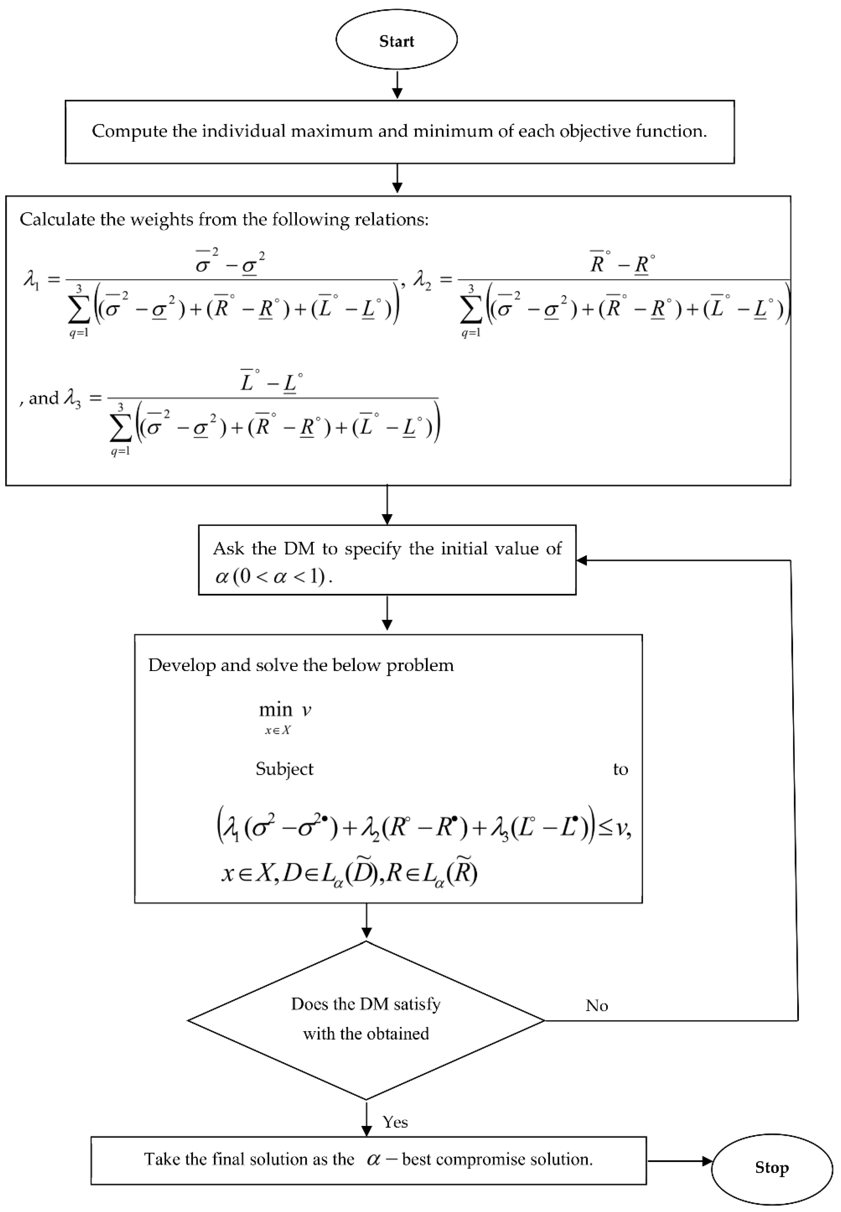
The steps of the procedure are as follows:
Step 1: Compute the independent maximum as well as minimum of all objective functions following the prescribed constraints for α = 0 , and α = 1 , respectively.
Step 2: Calculate the weights using the following relations:
λ 1 = σ ¯ 2 σ _ 2 q = 1 3 ( ( σ ¯ 2 σ _ 2 ) + ( R ¯ R _ ) + ( L ¯ L _ ) ) ,     λ 2 = R ¯ R _ q = 1 3 ( ( σ ¯ 2 σ _ 2 ) + ( R ¯ R _ ) + ( L ¯ L _ ) ) ,
and
λ 3 = L ¯ L _ q = 1 3 ( ( σ ¯ 2 σ _ 2 ) + ( R ¯ R _ ) + ( L ¯ L _ ) )
where σ ¯ 2 ,   R ¯ ,   L ¯ are individual maximum, and σ _ 2 ,   R _ ,   L _ are individual minimum.
Step 3: Consult the decision maker (DM) to point out an initial value of α   ( 0 < α < 1 ) .
Step 4: Develop and solve the below problem
                                              min   x X   v
Subject to
( λ 1   ( σ 2   σ 2 ) + λ 2 ( R R ) + λ 3 ( L L ) ) v ,   x X ,   D L α ( D ˜ ) ,   R L α ( R ˜ )
Step 5: If DM satisfies with the obtained results in Step 4, then terminate the procedure with the final solution as the α best compromise solution. Otherwise, go to Step 3.
A flow chart representation of the above interactive approach is also provided in Figure 1 below:

5. Numerical Experimentation

Consider a customer who recognized three mutual funds with attractive opportunities. From the past 5 years’ data, the dividend payments (USD) are shown in the following Table 1:
The weighting coefficients vector is equal to P = ( 0.197 ,   0.31 ,   0.493 ) T .
Step 1: The individual maximum and minimum can be calculated as in Table 2:
The individual maximum values are presented as follows
max   σ 2 ( x ,   D ) =   6 x 1 2 + 1.72 x 2 2 + 26.08 x 3 2 6.4 x 1   x 2 + 22.4 x 1   x 3 12.08 x 2   x 3
max R ( x ,   R ) =   9 x 1 + 6.4 x 2 + 10.2 x 3 ,
max   L ( x ,   p ) = 0.197 x 1 + 0.31 x 2 + 0.493 x 3
Subject to
x 1 + x 2 + x 3 = 1 . x 1 ,   x 2 ,   x 3 0 .
Hence, the individual maximum value of each objective is summarized in Table 3.
The investment stock is summarized in Table 4.
The individual minimum values are computed as follows:
min σ 2 ( x ,   D ) = 5.92 x 1 2 + 4.6 x 2 2 + 21.82 x 3 2 9.2 x 1 x 2 + 16.44 x 1 x 3 15 x 2 x 3 min R ( x ,   R ) = 5.6 x 1 + 5 x 2 + 8.6 x 3
min L ( x ,   p ) = 0.197 x 1 + 0.31 x 2 + 0.493 x 3
Subject to
x 1 + x 2 + x 3 = 1 . x 1 ,   x 2 ,   x 3 0 .
Thus, the individual minimum value of each objective is summarized in Table 5.
Step 2: The weights are computed as follows:
λ 1 = 0.824357 ,                                   λ 2 = 0.166184 ,                                                                 λ 3 = 9.45968 × 10 3
Step 3: Suppose that the DM selects α = 0.7 and based on the center of the intervals of confidence, we obtain the results as shown in Table 6 below.
The corresponding model is described as follows:
(0.7-EVL)′
min   σ 2 ( x ,   D ) = 12.2684 x 1 2 + 2.4886 x 2 2 + 49.27 x 3 2 5.1446 x 1 x 2 + 45.02 x 1 x 3 8.766 x 2 x 3
min   R ( x , R ) = 8.46 x 1 7.28 x 2 10.1 x 3
min   L ( x , p ) = 0.197 x 1 0.31 x 2 0.493 x 3
Subject to
x 1 + x 2 + x 3 = 1 , x 1 , x 2 , x 3 0 .
Step 4: Formulate and solve the following problem:
min   v
( 10.11354142 x 1 2 + 2.05149483 x 2 2 + 40.61606939 x 3 2 4.240987022 x 1 x 2 + 37.11255214 x 1 x 3 7.226313462 x 2 x 3 1.407780197 x 1 1.212752021 x 2 1.683122022 x 3 v ) 1.067972609 , x 1 + x 2 + x 3 = 1 , x 1 ,   x 2 , x 3 0 .
Suppose that the DM agreed with the α current solution, therefore we terminate the procedure and the α best compromise solution as in Table 7 below.
In order to estimate the fuzzy optimum value, let us follow Table 8 below.
E 1 = ( 5.6 ,   7.8 ,   9 ,   10 ) ,       E 2 = ( 4.4 ,   6 ,   7 ,   8 ) ,   E 3 = ( 8.2 ,   9.4 ,   10.4 ,   12 )
σ 11 2 = ( 44.6 , 8.4 ,   32.16 ,   80.64 ) ,     σ 22 2 = ( 34 , 10.2 ,   15.8 ,   47.44 ) , σ 33 2 = ( 18.4 , 28.84 ,   68.44 ,   128.76 ) , σ 12 2 = σ 21 2 = ( 51.6 , 21.6 ,   10.6 ,   40.8 ) , σ 13 2 = σ 31 2 = ( 48.6 , 0.2 ,   41.68 ,   89.16 ) ,   σ 23 2 = σ 32 2 = ( 69 , 27.6 ,   5.2 ,   43.24 ) .
Thereafter, we evaluate the parameter values of the proposed mathematical model as follows:
R ˜ = ( 5.40636 ,   6.97088 ,   7.99028 ,   9.1308 ) ,   σ ˜ 2 = ( 40.4603 ,   13.9806 ,   16.0218 ,   51.93105 )
The results show that the fuzzy return is R ˜ = ( 5.40636 ,   6.97088 ,   7.99028 ,   9.1308 ) , which means that the total expected return is greater than the value of 5.40636 and less than the value of 9.1308 , and the maximum return lies between 6.97088 , and 7.99028 . Furthermore, the fuzzy risk is σ ˜ 2 = ( 40.4603 ,   13.9806 ,   16.0218 ,   51.93105 ) , meaning that the total risk will be greater than 40.4603 and less than 51.93105 . In addition, the minimum risk lies between 13.9806 and 16.0218 .

6. Concluding Remarks

In the current study, we mathematically developed and solved an extended multi-objective portfolio selection problem which having liquidity as another objective function to be optimized besides the risk and return. The problem was formulated by incorporating fuzzy numbers in the risk matrix and return. A weighted Tchebycheff method was applied by defining relative weights and ideal targets for this problem. The advantage of the approach is the applicability in many real-world problems, which was illustrated through a numerical example problem in this research. In addition, the suggested methodology is more flexible where it permits the decision maker to select the targets in which he/she is interested. This is useful for further research and could be again developed as the generalized fuzzy numbers, neutrosophic numbers (Khalifa et al. [40]), etc.

Funding

This research received no external funding.

Institutional Review Board Statement

Not applicable.

Informed Consent Statement

Not applicable.

Data Availability Statement

No data were used in this manuscript.

Conflicts of Interest

The author declare that he has no conflict of interest.

References

  1. Simammora, I.; Sashanti, R. Optimization of fuzzy portfolio considering stock returns and downside risk. Int. J. Sci. Res. 2013, 5, 141–145. [Google Scholar]
  2. Zadeh, L.A. Fuzzy sets. Inf. Control 1965, 8, 338–353. [Google Scholar] [CrossRef]
  3. Dubois, D.; Prade, H. Fuzzy Sets and Systems: Theory and Applications; Academic Press: New York, NY, USA, 1980. [Google Scholar]
  4. Rommelfonger, H.; Hamuschecu, R.; Wolf, J. Linear programming with fuzzy objectives. Fuzzy Sets Syst. 1989, 29, 31–48. [Google Scholar] [CrossRef]
  5. Zhao, R.; Govind, R.; Fan, G. The complete decision set of the generalized symmetrical fuzzy linear programming problem. Fuzzy Sets Syst. 1992, 51, 53–65. [Google Scholar] [CrossRef]
  6. Zimmermann, J.H. Fuzzy Sets Theory and Its Application; Kluwer-Nijhoff Publishing: Leiden, The Netherlands, 1985. [Google Scholar]
  7. Ahmadini, A.; Ahmad, F. Solving intuitionistic fuzzy multi-objective linear programming problem under neutrosophic environment. AIMS Math. 2021, 6, 4556–4580. [Google Scholar] [CrossRef]
  8. Markowitz, H. Portfolio selection. J. Financ. 1952, 7, 77–91. [Google Scholar]
  9. Tanaka, H.; Ukuda, T.; Asal, K. Portfolio selection based on fuzzy probabilities distributions. Fuzzy Sets Syst. 2000, 111, 387–397. [Google Scholar] [CrossRef]
  10. Hassuike, T.; Katagiri, H.; Ishii, H. Portfolio selection problems considering fuzzy returns of future scenarios. Int. J. Innov. Comput. Inf. Control 2009, 4, 2493–2506. [Google Scholar]
  11. Ammar, E.E.; Khalifa, H.A. Fuzzy portfolio optimization: A quadratic programming approach. Chaos Solitons Fractal 2003, 18, 1042–1054. [Google Scholar] [CrossRef]
  12. Khalifa, H.A.; Zein, E.R.A. Fuzzy programming approach for portfolio selection problems with fuzzy coefficients. Int. J. Sci. Knowl. 2014, 4, 40–46. [Google Scholar]
  13. Luengo, E.A. Fuzzy mean-variance portfolio selection problems. Adv. Model. Optim. 2010, 12, 399–410. [Google Scholar]
  14. Bermudez, J.P.; Seguro, J.V.; Vercher, E. A Multi-objective genetic algorithm for cardinality constrained fuzzy portfolio selection. Fuzzy Sets Syst. 2012, 188, 16–26. [Google Scholar] [CrossRef]
  15. Xu, J.; Li, J. A class of stochastic optimization problems with one quadratic & several linear objective functions and extended portfolio selection model. J. Comput. Appl. Math. 2002, 146, 99–113. [Google Scholar]
  16. Chalco, C.Y.; Lodwick, W.A.; Bede, B. Single level constraint interval arithmetic, Fuzzy Sets and Systems. Int. J. Inf. Sci. Eng. 2014, 257, 146–168. [Google Scholar]
  17. Fard, O.S.; Ramezanzadeh, M. On fuzzy portfolio selection problems. A parametric representation approach. Complexity 2017, 9317924, 12. [Google Scholar]
  18. Glensk, B.; Madlener, R. Fuzzy portfolio optimization of power generation assets. Energies 2018, 2018, 3043. [Google Scholar] [CrossRef]
  19. Moghadam, M.A.; Ebrahimi, S.B.; Rahmani, D. A two-stage robust model for portfolio selection by using goal programming. J. Ind. Syst. Eng. 2019, 12, 1–17. [Google Scholar]
  20. Panwar, D.; Jha, M.; Srivastava, N. Optimization of risk and return using fuzzy Multiobjective linear programming. Adv. Fuzzy Syst. 2018, 2018, 4279236. [Google Scholar] [CrossRef]
  21. Qian, W.; Yin, M. Portfolio selection based on distance between fuzzy variables. Math. Probl. Eng. 2014, 2014, 403208. [Google Scholar] [CrossRef] [Green Version]
  22. Sardou, I.G.; Nazari, A.; Ghodsi, E.; Bagherzadeh, E. Optimal portfolio selection using the multi-objective fuzzy genetic method. Int. J. Econom. Financ. Manag. 2015, 3, 99–103. [Google Scholar]
  23. London, A.; Gena, I.; Banhelyi, B. Markowitz portfolio selection using various estimators of expected returns and filtering techniques for correlations metrics. Acta Polytech. Hung. 2018, 15, 217–229. [Google Scholar]
  24. Kumar, C.; Doja, D.N. A novel framework for portfolio selection model using modified ANFIS and fuzzy sets. Computers 2018, 7, 57. [Google Scholar] [CrossRef]
  25. Wei, H.; Xia, B.; Yang, Z.; Zhow, Z. Model and data- driven system portfolio selection based on value and risk. Appl. Sci. 2019, 9, 1657. [Google Scholar] [CrossRef]
  26. Chen, W.; Xu, W. A hybrid multi-objective bat algorithm for fuzzy portfolio optimization with real-world constraints. Int. J. Fuzzy Syst. 2019, 21, 291–307. [Google Scholar] [CrossRef]
  27. Chen, W.; Li, D.; Liu, Y. A novel hybrid ICA-FA algorithm for multi-period uncertain portfolio optimization model based on multiple criteria. IEEE Trans. Fuzzy Syst. 2019, 27, 1023–1036. [Google Scholar] [CrossRef]
  28. Chen, W.; Li, S.; Zhang, J.; Mehlawat, M.K. A comprehensive model for fuzzy multi-objective portfolio selection based on DEA cross-efficiency model. Soft Comput. 2020, 24, 2515–2526. [Google Scholar] [CrossRef]
  29. Mehlawat, M.K.; Gupta, P.; Kumar, A.; Yadav, S.; Aggarwal, A. Multi-objective fuzzy portfolio performance evaluation using data envelopment analysis under credibilistic framework. IEEE Trans. Fuzzy Syst. 2020, 28, 2726–2737. [Google Scholar] [CrossRef]
  30. Rangel, V.N.; Santillán, C.G.; Hernández-Marín, J.; Morales-Rodríguez, M.L.; Reyes, L.C.; Fraire-Huacuja, H.J. Parallel designs for metaheuristics that solve portfolio selection problems using fuzzy outranking relations. Int. J. Fuzzy Syst. 2020, 22, 2747–2759. [Google Scholar] [CrossRef]
  31. Deng, X.; Li, W. A novel probabilistic hesitant fuzzy portfolio selection model with value-at-risk and safety level of score. Eng. Comput. 2020, 38, 2137–2162. [Google Scholar] [CrossRef]
  32. Srizongkhram, S.; Manitayakul, K.; Suthamanondh, P.; Chiadamrong, N. Fuzzy chance-constrained integer programming models for portfolio investment selection and optimization under uncertainty. Int. J. Knowl. Syst. Sci. 2020, 11, 33–58. [Google Scholar]
  33. Zhang, X.; Hipel, K.; Tan, Y. Project portfolio selection and scheduling under a fuzzy environment. Memetic Comput. 2019, 11, 1–16. [Google Scholar] [CrossRef]
  34. Zhou, W.; Xu, Z. Score-hesitation trade-off and portfolio selection under intuitionistic fuzzy environment. Int. J. Intell. Syst. 2019, 34, 325–341. [Google Scholar] [CrossRef]
  35. Zhou, X.; Wang, L.; Liao, H.; Wang, S.; Lev, B.; Fujita, H. A prospect theory-based group decision approach considering consensus for portfolio selection with hesitant fuzzy information. Knowl. Based Syst. 2019, 168, 28–38. [Google Scholar] [CrossRef]
  36. Khalifa, H.A.; Alharbi, M.G.; Kumar, P. A new approach for the optimization of portfolio selection problem in fuzzy environment. Adv. Math. Sci. J. 2020, 9, 7171–7190. [Google Scholar] [CrossRef]
  37. Dymova, L.; Kaczmarek, K.; Sevastjanov, P.V. A new approach to the bi-criteria multi-period fuzzy portfolio selection. Knowl. Based Syst. 2021, 234, 107582. [Google Scholar] [CrossRef]
  38. Gong, X.; Min, L.; Yu, C. Multi-period portfolio selection under the coherent fuzzy environment with dynamic risk-tolerance and expected-return levels. Appl. Soft Comput. 2022, 114, 108104. [Google Scholar] [CrossRef]
  39. Mehrjerdi, Y.Z. A novel methodology for portfolio selection in fuzzy multi criteria environment using risk-benefit analysis and fractional stochastic. Numer. Algebra Control Optim. 2022, 12, 513–535. [Google Scholar] [CrossRef]
  40. Khalifa, H.A.; Majed, G.A.; Kumar, P. A new method for solving quadratic fractional programming problem in neutrosophic environment. Open Eng. 2021, 11, 880–886. [Google Scholar] [CrossRef]
Figure 1. Flow chart representation of the interactive approach.
Computers 11 00144 g001
Table 1. Investment stock.
Years
Funds12345
Investment 1(5, 8, 10, 11)(1, 3, 4, 5)(9, 11, 12, 13)(10, 12, 13, 14)(3, 5, 6, 7)
Investment 2(3, 5, 6, 7)(7, 8, 9, 10)(3, 5, 6, 7)(2, 4, 5, 6)(7, 8, 9, 10)
Investment 3(15, 16, 17, 19)(0, 1, 2, 3)(8, 10, 11, 12)(17, 18, 19, 21)(1, 2, 3, 5)
Table 2. Investment stock at α = 1 .
Years
Funds12345
Investment 110412136
Investment 269548
Investment 317111193
Table 3. Individual maximum values.
ObjectiveOptimal SolutionOptimum Value
σ 2 ( x ,   D ) (0.0000, 0.0000, 1.0000)26.0800
R ( x ,   R ) (0.0000, 0.0000, 1.0000)10.20000
L ( x ,   p ) (0.0000, 0.0000, 1.0000)0.4930
Table 4. Investment stock at α = 0 .
Years
Funds12345
Investment 1519103
Investment 2310327
Investment 31538171
Table 5. Individual minimum values.
ObjectiveOptimal SolutionOptimum Value
σ 2 ( x ,   D ) (0.4062, 0.5461, 0.0477)0.2853
R ( x ,   R ) (0.0000, 1.0000, 0.0000)5.0000
L ( x ,   p ) (1.0000, 0.0000, 0.0000)0.1970
Table 6. Investment stock at α = 0.7 .
Years
Funds12345
Investment 19.93.3511.3512.355.35
Investment 25.358.55.358.78.5
Investment 316.651.511.0518.652.65
Table 7. The α best compromise solution.
Optimal SolutionOptimum Value
x 1 = 0.0970 x 2 = 0.6688 x 3 = 0.2342 v = 0.2667
σ 2 = 3.2467 R = 8.0549 L = 0.3419
Table 8. Fuzzy covariance and expectation.
x i   1 2 x i   2 2 x i   3 2
1(40, 64, 100, 121)(15, 25, 36, 49)(240, 256, 289, 361)
2(3, 9, 16, 25)(56, 64, 81, 100)(0, 1, 4, 9)
3(99, 121, 144, 169)(15, 25, 36, 49)(80, 100, 121, 144)
4(120, 144, 169, 196)(8, 16, 25, 36)(306, 324, 361, 441)
5(15, 25, 36, 49)(56, 64, 81,100)(2, 4, 9, 25)
Sum(277, 363, 465, 560)(150, 194, 259, 334)(628, 685, 784, 980)
x i   1   x i   2 x i   1   x i   3 x i   2   x i   3
1(25, 40, 60, 77)(80, 128, 170, 209)(48, 80, 102, 133)
2(8, 24, 36, 50)(1, 3, 8, 15)(7, 8, 18, 30)
3(45, 55, 72, 91)(90, 110, 132, 156)(30, 50, 66, 84)
4(40, 48, 65, 84)(180, 216, 247, 294)(36, 72, 95, 126)
5(24, 40, 54, 70)(6, 10, 18, 35)(14, 16, 27, 50)
Sum(142,207, 287,372)(357, 467, 575, 709)(135,226, 308, 423)
Publisher’s Note: MDPI stays neutral with regard to jurisdictional claims in published maps and institutional affiliations.

