Article

Prediction of Severity of COVID-19-Infected Patients Using Machine Learning Techniques

1
Department of Computer Science, College of Computers and Information Technology, Taif University, Taif 26571, Saudi Arabia
2
Deanship of University Development, Taif University, Taif 26571, Saudi Arabia
3
Rehabilitation Sciences Department, College of Applied Medical Sciences, Najran University, Najran 66446, Saudi Arabia
*
Author to whom correspondence should be addressed.
Computers 2021, 10(3), 31; https://doi.org/10.3390/computers10030031
Submission received: 25 January 2021 / Revised: 3 March 2021 / Accepted: 4 March 2021 / Published: 9 March 2021

Abstract

:
Precisely assessing the severity of persons with COVID-19 at an early stage is an effective way to increase the survival rate of patients. Based on the initial screening, to identify and triage the people at highest risk of complications that can result in mortality risk in patients is a challenging problem, especially in developing nations around the world. This problem is further aggravated due to the shortage of specialists. Using machine learning (ML) techniques to predict the severity of persons with COVID-19 in the initial screening process can be an effective method which would enable patients to be sorted and treated and accordingly receive appropriate clinical management with optimum use of medical facilities. In this study, we applied and evaluated the effectiveness of three types of Artificial Neural Network (ANN), Support Vector Machine and Random forest regression using a variety of learning methods, for early prediction of severity using patient history and laboratory findings. The performance of different machine learning techniques to predict severity with clinical features shows that it can be successfully applied to precisely and quickly assess the severity of the patient and the risk of death by using patient history and laboratory findings that can be an effective method for patients to be triaged and treated accordingly.

1. Introduction

The novel COVID-19 (severe acute respiratory syndrome coronavirus-2) disease was detected in Wuhan city, Hubei province and reported to the WHO Country Office in China on 31 December 2019; since then it has spread to countries and territories around the whole world [1]. COVID-19 is a ribonucleic acid (RNA) virus and a member of the Coronavirus family that resides in mammals and birds. In the past, the members of these viruses have also spilled over between species (mammals and birds to humans) [1,2]. The common symptoms of coronaviruses are the common cold, fever, and a sore throat, but vary significantly with the strain and varieties of virus, like a notable symptom in the COVID-19 being Tachypnea [3]. The mortality rates significantly vary with varieties of virus; SARS has the highest mortality rate however the common flu has the lowest rate. The severity scale of COVID-19 infection varies from mild to critical [4]. The Chinese Center for Disease Control and Prevention report on the severity of the disease features Mild (80.9%), Severe disease (13.8%), and Critical disease (4.7%) with a fatality rate of 2.3 percent [4,5]. Prediction of the severity of the patient and the risk of death by initial screening and testing results manually is a challenging problem. Hence, it has become an urgent yet challenging problem to identify patients with high risk of death from the infectious population using testing data with the assistance of artificial intelligence. The developed prognostic model based on artificial intelligence could instigate early treatment to critical patients and thus potentially minimize the mortality. The majority of health experts amicably endorse that testing is the essential component to control the outbreak. The PCR test is the front-line test for COVID-19 because it directly detects the presence of the virus RNA. The Lung CT is also proposed by Ali et al. as an effective method of early detection of infection [6]. After test confirmation of infection, the patient needs to go for clinical testing to evaluate the risk factors for severe illness. In a study of patients who have confirmed symptoms of COVID-19, serious illness is found to occur in patients of all ages, but it occurs primarily in patients with advanced age or underlying medical disorders. Thus, the patient history of medical complexities, medical reports and clinical characteristics of the patients can be an effective technique to predict the severity of illness [7]. Researchers have made several efforts to establish correlations between clinical characteristics and medical complexities with severity of illness. There are hundreds of clinical characteristics associated with medical complexities that can influence the severity of illness. Therefore, advance features selection techniques are required to identify those features which contribute most to the severity of illness in which we are interested in, as having irrelevant clinical features increases the chances of error in prediction significantly. Plenty of feature selection methods are available in the literature. Relief-based algorithms (RBAs) developed by Kira and Rendell in 1992 [8], are one of the most prominent feature selection algorithms in the course of machine learning. Relief algorithms can efficiently identify the relevant feature from the set of clinical features which contribute to the severity of illness and have strong dependencies between them. Relief algorithms ranked the applied features or input variables according to their contribution in critical illness of the infected patient.
Precisely and early assessing the severity of the COVID-19-infected patients and the risk of death is very important for the categorizing patients, which would enable patients to be sorted and treated accordingly to receive appropriate clinical management with optimum use of medical facilities and prevent the occurrence of over handling or under handling of patient care, thus potentially reducing mortality. In particular, where an outbreak occurs and medical resources are relatively scarce, it is necessary to conduct an assessment of the severity and treatment, thereby optimizing the allocation of rescue resources, and to prevent the appearance of overtreatment or undertreatment. In clinical characteristics-based medical diagnosis, Artificial intelligence (AI) techniques such as Fuzzy logic, Genetic algorithms (GA), Decision Trees, Support Vector Machines (SVM), Artificial Neural Networks (ANNs), and Deep learning have gained popularity in the field of health care for detection, identification, and estimation of various medical problems [9,10,11].
In this paper, our study was to apply and evaluate machine learning techniques for precise and early prediction of the severity of the COVID-19-infected patient. The patient history and clinical findings were used to train different supervised machine learning techniques, and a portion of data sets were used to evaluate the effectiveness of the proposed methods. The rest of the paper is organized as follows, the materials and methods are discussed in Section 2. In Section 3, the proposed methodology is evaluated on real-life COVID datasets. Section 4 present the conclusions.

2. Results

The efficiency of the machine learning techniques were tested by a variety of machine learning techniques. The 80 samples of the data set were randomly partitioned into a training data set and a testing data set, the training data set consisting of 62.5% samples and remaining 37.5% samples used for testing. The normalized inputs were fed to each machine learning model. Various performance measures [12] like Accuracy, Sensitivity, Specificity, Precision, F_Score and G-mean error were used to evaluate the performance capability of each machine learning techniques using 10 cross validations.
Accuracy = (True positive (TP)+ True negative (TN))/(Total Samples).
Recalls (Sensitivity) = True positive (TP)/(True positive (TP)+ False negative (FN)).
Specificity = True negative (TN)/(True negative (TN)+ False positive (FP)).
Precision = True positive (TP)/(True positive (TP)+ False positive (FP)).
F_Score = 2* ((Precision*Recall)/(Precision + Recall)).
G-mean = Sqrt (Recalls * Specificity).
where,
True positive (TP): Prediction of the severity is +ve and Patient is severe.
False positive (FP): Prediction of the severity is +ve and Patient is not severe.
True negative (TN): Prediction of the severity is −ve and Patient is not severe.
False negative (FN): Prediction of the severity is −ve and Patient is severe.

2.1. Multilayer Perceptron

In the performance evaluation of the multi-layer perceptron (MLP), twenty neurons were used in the hidden layer. Performance evaluation of the Multilayer perceptron was done using Levenberg–Marquardt backpropagation (“trainlm”), Scaled conjugate gradient backpropagation (“trainscg”) and Bayesian regularization backpropagation (“trainbr”). The average time taken in performance evaluation was 2.338429 s. The performance evaluation of multilayer perceptron neural network is given in Table 1. The confusion matrix obtained using the multilayer perceptron with “trainlm”, “trainbr” and “trainscg” is shown in Figure 1.

2.2. Radial Basis Neural Network

In the performance evaluation of RBF, fifty neurons were used in the hidden layer. Performance evaluation of the RBF was done using different levels of spread, normal spread = 1, small spread = 0.5 and large spread = 10. The average time taken in performance evaluation was 1.370280 s. The performance evaluation of the RBF network is given in Table 2. The confusion matrix obtained using the multilayer perceptron with “trainlm”, “trainbr” and “trainscg” are shown in Figure 2.

2.3. General Regression Neural Network

In the performance evaluation of the General Regression Neural Network (GRNN), fifty neurons were used in the hidden layer. Performance evaluation of the GRNN was done using different levels of spread, normal spread = 1, small spread = 0.5 and large spread = 5. The average time taken in performance evaluation was 1.109263 s. The performance evaluation of the GRNN is given in Table 3. The confusion matrix obtained using GRNN different levels of spread is shown in Figure 3.

2.4. Support Vector Machine

In an evaluation of performance of the SVM, Linear, Polynomial and RBF kernel function were used to map the training data into kernel space. The average time taken in performance evaluation was 2.234734 s. The performance evaluation of the Support Vector Machine is given in Table 4. The confusion matrix obtained using the SVM with “linear”, “quadratic” and “rbf” kernels are shown in Figure 4.

2.5. Random Forest

In the performance evaluation of the Random Forest method, a set of a hundred classification decision trees was used as base learners for the Random forest. The maximum split or each tree was fixed at five times. The ensemble of classification trees used LPBoost, AdaBoostM1 and bag methods. The average time taken in performance evaluation was 2.554221 s. The performance evaluation of the Random forest method is given in Table 5. The confusion matrix obtained using “LPBoost”, “GentleBoost”, “AdaBoostM1”, “RobustBoost”, “TotalBoost”, “RUSBoost” and “Bag” ensemble methods in the Random forest are shown in Figure 5.

3. Discussion

All the described and implemented machine learning techniques showed a high accuracy and precision and a smaller amount of error sensitivity or recalls in the prediction of the severity of COVID-19 patients. The best performance in all the applied methods is given by with Random forest method with the ensemble of decision trees using “LPBoost” “GentleBoost” “AdaBoostM1”. The next best performance was recorded by the multilayer perceptron neural network training with Bayesian regularization algorithms. The performance of RBF showed poorest results, especially in the measure of sensitivity. The performance of the GRNN and SVM with different parameters was fair. The performance measures of the machine learning techniques show the potential for accurate assessment of severity for COVID-19-infected patients. The present research demonstrates that machine learning can be an effective method to assess the severity of the patient and the risk of death precisely and quickly by using patient history and the laboratory findings which would enable patients to be sorted and treated accordingly to receive appropriate clinical management with optimum use of medical facilities. The random forest method proved to be the most efficient and reliable machine learning technique for severity prediction.

4. Materials and Methods

The experiment was performed on a computer with a six core Core i7 (7th Gen.) processor, 16 GB RAM, and 8 GB graphics memory of a NVIDIA GeForce GTX-1070 GPU. MATLAB R2017a (64-bit). The Materials and Methods include a short description of the data sets, details on the feature selection process and a brief introduction to the various machine learning techniques and training algorithms used in the prediction of severity.

4.1. Dataset

All the proposed machine learning methodologies are implemented with the data obtained from the research article published by Zhenhuan Cao et al. [13] on page 6, “S1 data”. The obtained clinical data were reviewed by a team of physicians at Peking University Clinical Research Institute. The data set information includes demographic data, signs and symptoms, medical history and treatment measures of the COVID-infected patients. The data sets consist of 52 features. The clinical features include patient physical properties, Sign and Symptoms, Admission time frame, chronic medical illness, Chronic obstructive pulmonary disease, Oxygen saturation, Systolic blood pressure, Smoking history, Pulse, Respiratory rate, Pneumonia manifestations, various blood properties and treatment measures. The performance of machine learning models depends upon the quality of data. Preprocessing was conducted on the available data sets which included handling the missing values and normalization.

4.2. Feature Selection

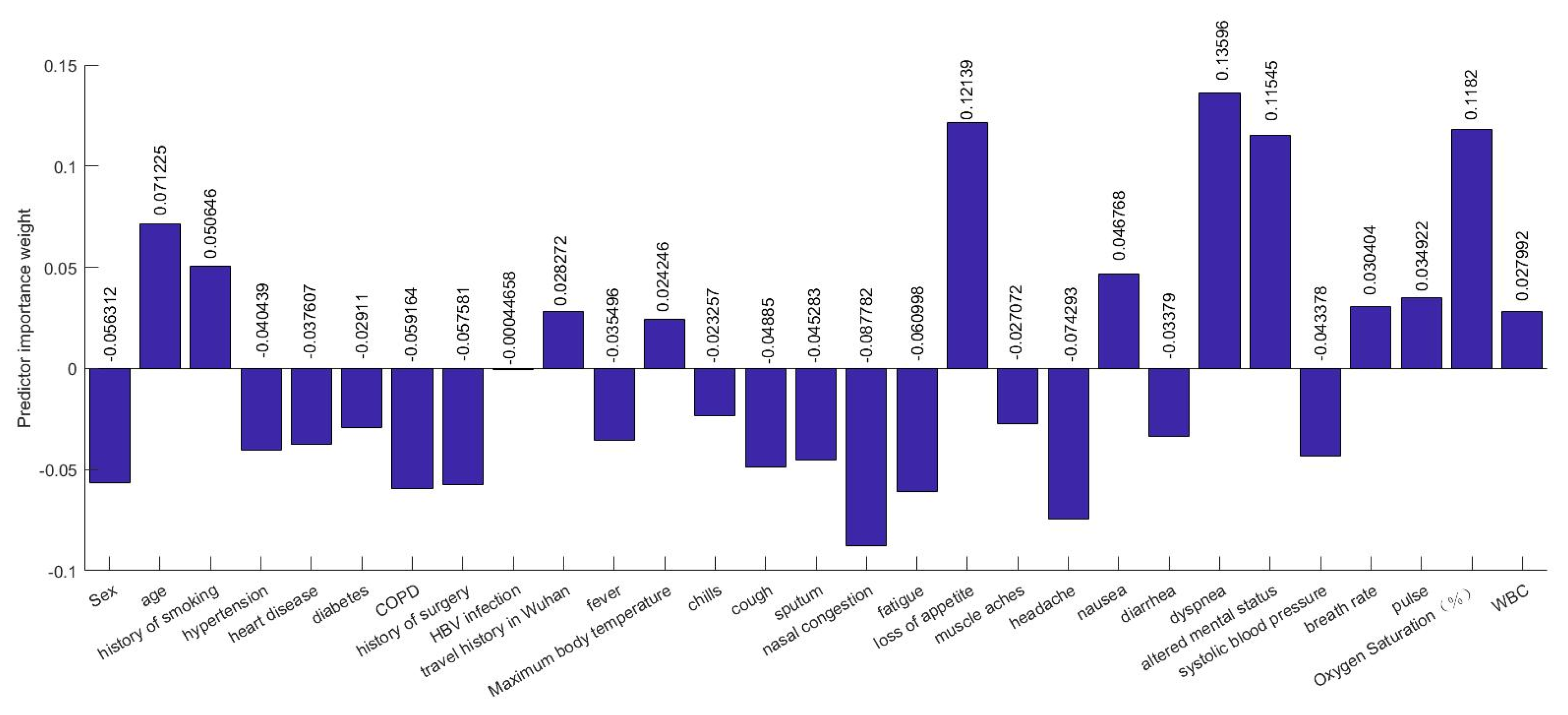
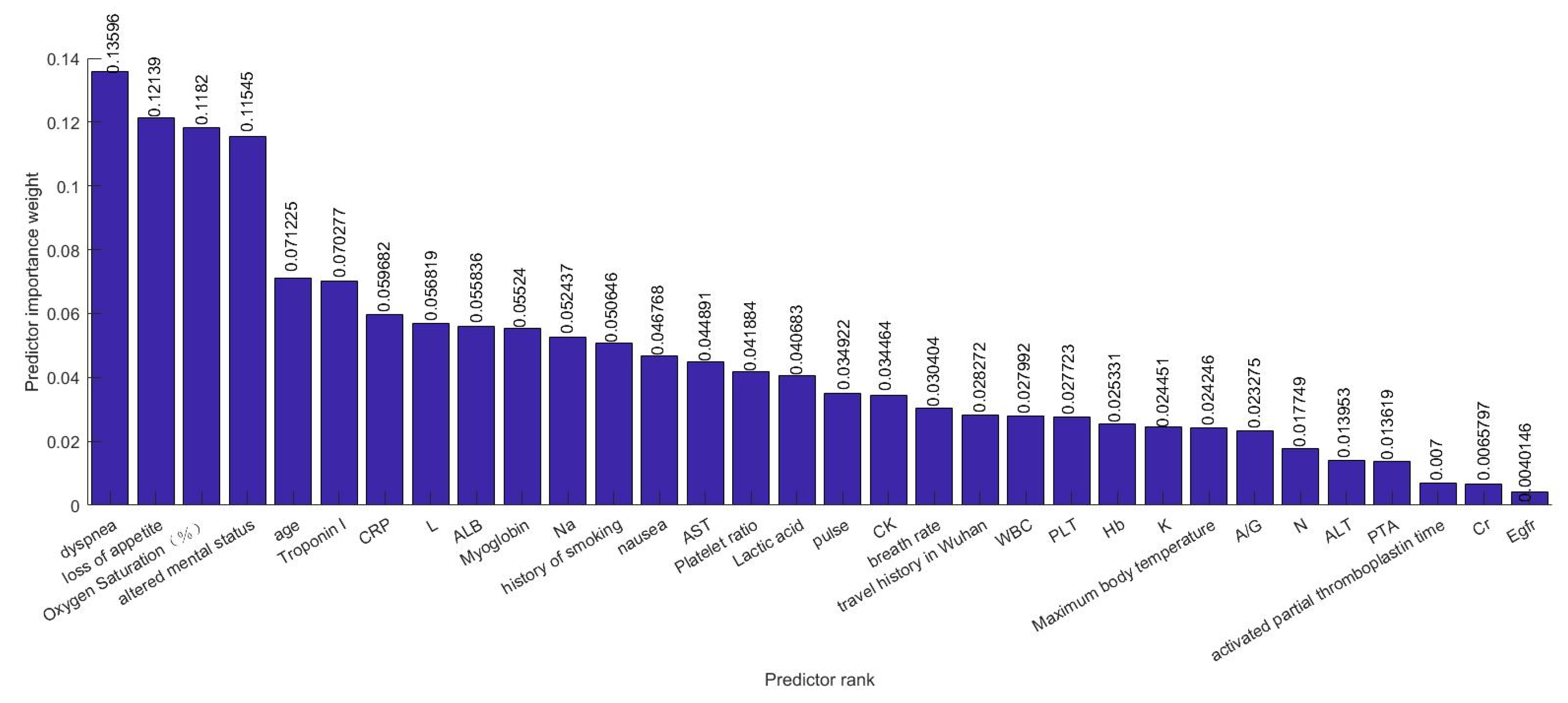
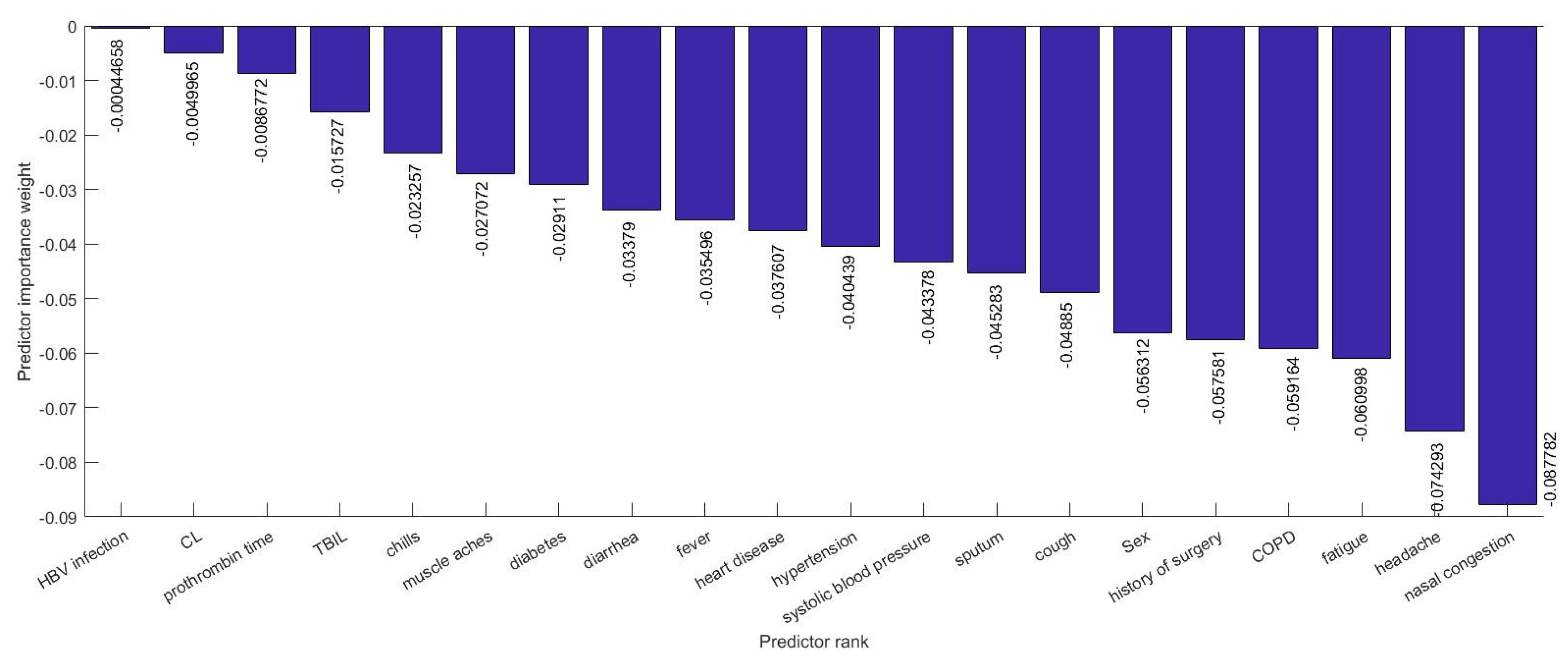
Several efforts have been made to establish correlations between clinical characteristics and medical complexities with the severity of illness. There are hundreds of clinical characteristics associated with medical complexities that can influence the severity of illness. Therefore, advanced feature selection techniques are required to identify those features which contribute most to the severity of illness in which we are interested, as having irrelevant clinical features increases the chances of error in prediction significantly. A number of methods for feature selection are available in the literature. G. Chandrashekar and F. Sahin concluded in their survey [14] that a feature selection algorithm can be designed based on Filter, Wrapper and Embedded methods and can be selected based on the number of reduced features, classification accuracy, simplicity, stability, storage and computational requirements. Relief-based algorithms (RBAs) developed by Kira and Rendell in 1992 [8], are one of the most prominent feature selection algorithms in the area of machine learning. While many feature selection algorithms assume conditional independence of the clinical features for estimating the quality of the clinical feature, Relief algorithms do not make this assumption. Relief algorithms can efficiently identify the relevant feature from the set of clinical features which contribute to the severity of illness and have strong dependencies between them. The feature selection was adopted on the training data and testing data were left aside for the classification. Relief algorithms compute the weights of the applied 52 features or input variables according to their contribution in critical illness of the infected patient as shown in Figure 6 and Figure 7. Selected 32 clinical features ranked based on their importance in the prediction of the severity are shown in Figure 8. The discarded 20 clinical features as they have a negative contribution in the prediction process are shown in Figure 9.

4.3. Machine Learning Methodologies

Three types of neural network architecture, Support vector regression, which is a kernel method; and Random forest regression, which is based on decision trees, are implemented in the present research. The brief methodology, working procedure, and the difference are given below.

4.3.1. Multilayer Perceptron

An artificial neural network is a machine learning architecture or model inspired by the human brain. The neural network is a combination of nodes or neurons. The most popular neural network is the feed-forward neural network or multi-layer perceptron (MLP) neural network [15]. Both architectures names are used interchangeably and widely used in neural network studies. Every layer is connected in series with nodes or neurons from input to output in multi-layer perceptron (MLP). The neural network comprises three types of layers, the input layer, the hidden layer and finally an output layer. The number of hidden layers can be manipulated, and the complexity of the neural network architecture increases with the increase in the number hidden layers and the number of neurons in the hidden layer.
The inputs are given in the first layer (input layer) and the outputs are at the last layer (output layer). The hidden layer has two functions; first is an aggregation function and another is an activation function. The aggregation function calculates the weighted arithmetic mean of the received input from the input layer using initial/update weights and bias. After that, the activation function is applied on that aggregated net. Activation functions could be linear and nonlinear (i.e., threshold, tan-sigmoid, log sigmoid etc.) depending on the application of neural network. However, most of time in the multi-layer perceptron (MLP) nonlinear activation functions are used because, from the nonlinear value, a deterministic or binary value can be achieved using various methods (such as maximum likelihood criteria). The information flows in a forward direction in the feed forwarded network and error correction is done by a backpropagation algorithm. The method works iteratively to minimize the error and optimized weight and bias.
H = Φ ( W 0 + i = 1 N ( W i X i ) )
Y = Φ ( V 0 + j = 1 M ( V i H i ) )
E ( w ) = 1 2 k = 1 P ( Y k T k ) 2
E   ( w ) is the error function.
Y k is an output vector
T k is a target vector.
Φ is an activation function.
W 0 is a bias.
W i are a weight vector.
X i are an input vector.
U 0 is a bias of the hidden layer.
U i is a weight vector of the hidden layer.
H is an output of the hidden layer.
H i is an input vector of the hidden layer.
Y is a final output.
In the artificial neural network, the error function is used to minimize the error using back-propagation. The target vector is subtracted from the output vector. In addition, the weight and bias are updated. The output of the MLP is calculated by the sum of the weight vector of the hidden layer and the input vector of the hidden layer with the bias of the hidden layers. This is done after using the linear or nonlinear activation function. Outputs of the hidden layers are calculated by the summation of the Input weight vector and the input vector with the linear or nonlinear activation function.

4.3.2. Radial Basis Function Network

The radial basis function, which is a Gaussian distribution-based kernel function, is used in a neural network to predict the output [16]. It is a nonlinear function used as an activation function in the neural network. RBF NN has three layers. The first layer is an input layer. The second is a hidden layer with a nonlinear RBF activation function. The last layer is an output layer which is linear. Basically, RBF converts the input matrix into the Gaussian form.
V ( X n ) = e ( X n 2 / 2 )
This function can be shifted to an arbitrary Centre, X = a where “a” is the mean of the input vector and with standard deviation “σ”
V ( X n a σ ) = e ( X n a ) 2 / 2 σ 2 )
Here V (Xn) is the input matrix of the features. Then, we calculate the output of the hidden layer and then calculate the final output.
H = Φ ( W 0 + i = 1 N ( W i V ( X i ) ) )
Y = Φ ( U 0 + j = 1 M ( U i H i ) )
Φ is an activation function.
W 0 is a bias.
W i is a weight vector.
X i is an input vector.
U 0 is a bias of the hidden layer.
U i is a weight vector of the hidden layer.
H is an output of the hidden layer.
H i is an input vector of the hidden layer.
Y is a final output.
The output of the hidden neuron is calculated based on the distance between the Centre of each activation or basis function and the input of each hidden neuron.

4.3.3. General Regression Neural Network

The General Regression Neural Network (GRNN) is a relatively newly-defined architecture of a neural network [17]. In the GRNN, a nonlinear arbitrary function is optimized as a relation between output and input data through training examples. In the GRNN, an iterative training procedure is not required like in the multilayer perceptron (MLP). The prediction of the continuous variable is the best suited case to the GRNN. Since the GRNN is a variation of an RBF neural network, it also uses kernel regression. Prediction of the dependent variable occurs from the independent variable of training examples. The GRNN minimizes the RMSE to zero and it is one of the merits of GRNN. It estimates the joint PDF of the independent and dependent variables from the training examples. The joint PDF is made from the training data, so no presumption is followed, and this makes it more general. It also gives the condition that, if the training set becomes larger, the error approaches to zero.
E [ y / x ] = y . f ( x , y ) d y f ( x , y ) d y
Y is a predict output vector.
X is an input vector.
E [ y / x ] is an expected value of output.
F ( x ,   y ) is the joint density function of x and y.
y m = n = 1 N ( h n . w n m ) n = 1 N ( h n )
w n m is a weight vector.
h n is an output of hidden layer.
h n = e D n 2 . s p r e a d 2
D n = ( x k n ) T ( x k n )
X is an input vector.
K is the training vector.
Spread is a constant that are used to control the size of the receptive region.

4.3.4. Support Vector Machine

The Support Vector Machine (SVM) was introduced by Vapnik et al. [18] in 1997, and was based on statistical learning theory. In the SVM, the goal is to find an approximation function that tries to predict the dependent output variable (Y) on the basis of independent input variables (X) such that the deviation from the predicted output value and target value is less than or equal to an error measure until the error is tolerated (ε). We assumed an approximation function f(x) which tries to predict the output (Y) of the model. For simplicity, we can take a linear basis function given as
f ( x ) = w , x + b ,   w h e r e   w ϵ X ,   b   ϵ   R
In this case, ascertaining that the approximation function provides a good prediction; the norm of w, w 2 = w , w , should be minimized. Then the cost function to optimize will be
m i n 1 2 w 2
s u b j e c t   t o   { y i w , x i b ε w , x i + b y i ε

4.3.5. Random Forest Regression

Leo Breiman proposed the Random forest scheme in the 2000’s for building an ensemble method for prediction by using a decision trees forest which grows in randomly selected data sub-spaces. Breiman demonstrated that, by using ensembles of trees, classification and regression accuracy can be improved. In the proposed scheme, each tree is produced in the ensemble in accordance with a random parameter. The final prediction is computed by aggregation of the output by each individual tree. The individual random trees are generated in the following way [19]
  • A coordinate of X = ( X 1 , X 2 , .. , X d ) is selected at each tree node, with the j t h feature which has the selection probability of p n j ( 0 , 1 ) .
  • After obtaining the selected coordinate, the split is at the midpoint of the chosen side of every node.
For every random tree r n ( X , Θ ) , the outputs average overall Y i , for which the corresponding vectors X i land in the same cell of the random partition as X .

4.4. Training Functions

There are varieties of training algorithms available for neural network from gradient descent to quasi-newton [20]. The basic function of the training algorithm is to minimize the cost function. The cost function in a neural network is a composite of the error term and the regularization term. The error is a difference in calculated response versus the real response and a regularization term is added to prevent overfitting. Therefore, cost function is dependent on adaptive parameters (bias and weights) and collectively these parameters make a n-dimensional loss function. The task is to find the global minima of the cost function. The first derivative of the cost function is combined as a gradient as
i f ( w ) = d f d w i   f o r   ( i = 1 , 2 , , n )
The second derivatives are combined as the Hessian matrix.
H i , j f ( w ) = d f d w i . d w j   f o r   ( i , j = 1 , 2 , . , n )
However, there are many algorithms for training neural network, but in the present study the three most widely used and efficient algorithms are applied (i.e., Bayesian regularization, the scale conjugate gradient, and the Levenberg–Marquard algorithm) and compared.

4.4.1. Levenberg–Marquard (“Trainlm”)

The LM algorithm is also known as the damped least square method and it works when the loss function can be represented in the sum of squared errors. Instead of computing the Hessian matrix, the LM algorithm works with a gradient and a Jacobian matrix.
f = e i 2 ,   f o r   i = 0 , 1 , m
M is the number of observations in data.
The Jacobian matrix can be defined by the function containing derivative of errors with respect to weights.
J i , j f ( w ) = d e i d w j   f o r   ( i = 1 , 2 , m   &   j = 1 , 2 , n )
The gradient vector is given by:
f = 2 J T . e
and the Hessian matrix can be approximated by
H f 2 J T . J + λ I
where λ is the damping factor and I is an identity matrix.
The parameter improvement process in the LM algorithm is given by
w i + 1 = w i ( J i T . J i + λ I ) - 1 . ( 2 . J i T . e i ) ,   f o r   i = 0 , 1 ,
The initial value parameter λ is set to be large so that start updates are small in the gradient descent direction. As the error decreases, λ is decreased. This process accelerates the convergence speed to the minimum.

4.4.2. Bayesian Regularization (“Trainbr”)

Bayesian regularization works after the Levenberg–Marquard algorithm. It minimizes the combination of the sum of squared error and the Jacobian matrix of weight and bias.
f ( w ) = α w i 2 + β e 2
where α and β are parameters of the cost function and they are decided using Bayes’ theorem of conditional probability given by
P ( A | B ) = P ( B | A )   P ( A ) P ( B )
This function is optimized to find the appropriate weight space. This could be done by maximizing the posterior probability function
P ( α , β | D , M ) = P ( D | α , β , M )   P ( α , β | M ) P ( D | M )
In the given expression, α and β are optimization factors.
D is distributed weight.
M is a type of the neural network.
( α , β | M ) is the uniform prior density.
P ( D | α , β , M ) is the likelihood function of “ D ” for a given α , β , and   M .
The objective is to find the best values for α and β . Then, the algorithm goes into the LM procedure where calculations are done in the Hessian matrix. Finally, the new values of α and β are found and the procedure continues until convergence.

4.4.3. Scale Conjugate Gradient (“Trainscg”)

In the scale conjugate gradient, the convergence towards the minima through the gradient is accelerated in the conjugate direction of the Hessian matrix. Considered as direction vector and if starting with initial parameter direction vector w 0 , then d 0 = g 0 . Then, a sequence of training vectors is constructed.
d i + 1 = g i + 1 + d i . y i   ,   f o r   i = 0 , 1 ,
where y is a conjugate parameter and can be found in various ways. The parameter improvement process is given by:
w i + 1 = w i + d i . η i ,   f o r   i = 0 , 1 , .
Here, η is the learning rate.

Author Contributions

Conceptualization, A.A. (Aziz Alotaibi) and M.S.; methodology, A.A. (Aziz Alotaibi); software, M.S.; validation, A.A. (Aziz Alotaibi), M.S., A.A. (Adel Alshahrani); formal analysis, A.A. (Adel Alshahrani); investigation, A.A. (Aziz Alotaibi); resources, M.S.; data curation, A.A. (Adel Alshahrani); writing—original draft preparation, A.A. (Aziz Alotaibi) and M.S.; writing—A.A. (Aziz Alotaibi) and A.A. (Adel Alshahrani); visualization, M.S.; supervision, A.A. (Aziz Alotaibi); project administration, A.A. (Aziz Alotaibi); funding acquisition, A.A. (Aziz Alotaibi), M.S. and A.A. (Adel Alshahrani). All authors have read and agreed to the published version of the manuscript.

Funding

This work was supported by the Research Group Program funded by the Deanship of Scientific Research, Taif University, K.S.A., under grant number (1-441-34).

Institutional Review Board Statement

Not applicable.

Informed Consent Statement

Not applicable.

Data Availability Statement

The data presented in this study are available in [11].

Conflicts of Interest

The authors declare no conflict of interest.

References

  1. Zhu, N.; Zhang, D.; Wang, W.; Li, X.; Yang, B.; Song, J.; Zhao, X.; Huang, B.; Shi, W.; Lu, R.; et al. A novel coronavirus from patients with pneumonia in China, 2019. N. Engl. J. Med. 2020. [Google Scholar] [CrossRef] [PubMed]
  2. Su, S.; Wong, G.; Shi, W.; Liu, J.; Lai, A.C.K.; Zhou, J.; Liu, W.; Bi, Y.; Gao, G.F. Epidemiology, Genetic Recombination, and Pathogenesis of Coronaviruses. Trends Microbiol. 2016, 24, 490–502. [Google Scholar] [CrossRef] [PubMed] [Green Version]
  3. Huang, C.; Wang, Y.; Li, X.; Ren, L.; Zhao, J.; Hu, Y.; Zhang, L.; Fan, G.; Xu, J.; Gu, X.; et al. Clinical features of patients infected with 2019 novel coronavirus in Wuhan, China. Lancet 2020. [Google Scholar] [CrossRef] [Green Version]
  4. Wu, Z.; McGoogan, J.M. Characteristics of and Important Lessons from the Coronavirus Disease 2019 (COVID-19) Outbreak in China: Summary of a Report of 72314 Cases from the Chinese Center for Disease Control and Prevention. JAMA-J. Am. Med. Assoc. 2020, 323, 1239–1242. [Google Scholar] [CrossRef] [PubMed]
  5. Dai, M.; Liu, D.; Liu, M.; Zhou, F.; Li, G.; Chen, Z.; Zhang, Z.; You, H.; Wu, M.; Zheng, Q.; et al. Patients with cancer appear more vulnerable to SARS-CoV-2: A multicenter study during the COVID-19 outbreak. Cancer Discov. 2020. [Google Scholar] [CrossRef] [PubMed]
  6. Asadollahi-Amin, A.; Hasibi, M.; Ghadimi, F.; Rezaei, H.; SeyedAlinaghi, S.A. Lung involvement found on chest CT scan in a pre-symptomatic person with SARS-CoV-2 infection: A case report. Trop. Med. Infect. Dis. 2020, 5, 56. [Google Scholar] [CrossRef] [PubMed]
  7. Yan, L.; Zhang, H.-T.; Xiao, Y.Y.; Wang, M.; Sun, C.; Liang, J.; Li, S.; Zhang, M.; Guo, Y.; Xiao, Y.Y.; et al. Prediction of criticality in patients with severe COVID-19 infection using three clinical features: A machine learning-based prognostic model with clinical data in Wuhan. medRxiv 2020. 2020.02.27.20028027. [Google Scholar]
  8. Kira, K.; Rendell, L.A. Feature selection problem: Traditional methods and a new algorithm. In Proceedings of the Proceedings Tenth National Conference on Artificial Intelligence, San Jose, CA, USA, 12–16 July 1992; pp. 129–134. [Google Scholar]
  9. Rida, I.; Al-Maadeed, N.; Al-Maadeed, S.; Bakshi, S. A comprehensive overview of feature representation for biometric recognition. Multimed. Tools Appl. 2020. [Google Scholar] [CrossRef]
  10. Rida, I.; Al Maadeed, S.; Jiang, X.; Lunke, F.; Bensrhair, A. An Ensemble Learning Method Based on Random Subspace Sampling for Palmprint Identification. In Proceedings of the ICASSP, IEEE International Conference on Acoustics, Speech and Signal Processing - Proceedings, Calgary, AB, Canada, 15–20 April 2018; pp. 2047–2051. [Google Scholar]
  11. Shamim, M.Z.; Syed, S.; Shiblee, M.; Usman, M.; Zaidi, M.; Ahmad, Z.; Muqeet, M.; Habeeb, M. Detecting benign and pre-cancerous tongue lesions using deep convolutional neural networks for early signs of oral cancer. Basic Clin. Pharmacol. Toxicol. 2019, 125, 184–185. [Google Scholar]
  12. Indola, R.P.; Ebecken, N.F.F. On extending F-measure and G-mean metrics to multi-class problems. WIT Trans. Inf. Commun. Technol. 2005, 35, 10. [Google Scholar]
  13. Cao, Z.; Li, T.; Liang, L.; Wang, H.; Wei, F.; Meng, S.; Cai, M.; Zhang, Y.; Xu, H.; Zhang, J.; et al. Clinical characteristics of Coronavirus Disease 2019 patients in Beijing, China. PLoS ONE 2020, 15, e0234764. [Google Scholar] [CrossRef]
  14. Chandrashekar, G.; Sahin, F. A survey on feature selection methods. Comput. Electr. Eng. 2014. [Google Scholar] [CrossRef]
  15. Rumelhart, D.; Hinton, G.; Williams, R. Learning Internal Representations By Error Propagation (original). Explor. Micro-Struct. Cogn. 1986, 1. [Google Scholar]
  16. Schwenker, F.; Kestler, H.A.; Palm, G. Three learning phases for radial-basis-function networks. Neural Netw. 2001. [Google Scholar] [CrossRef]
  17. Specht, D.F. A General Regression Neural Network. IEEE Trans. Neural Netw. 1991. [Google Scholar] [CrossRef] [PubMed] [Green Version]
  18. Cortes, C.; Vapnik, V. Support-Vector Networks. Mach. Learn. 1995. [Google Scholar] [CrossRef]
  19. Breiman, L. Random forests. Mach. Learn. 2001. [Google Scholar] [CrossRef] [Green Version]
  20. Suk, H.I. An Introduction to Neural Networks and Deep Learning. In Deep Learning for Medical Image Analysis; Academic Press: Cambridge, MA, USA, 2017; ISBN 9780128104095. [Google Scholar]
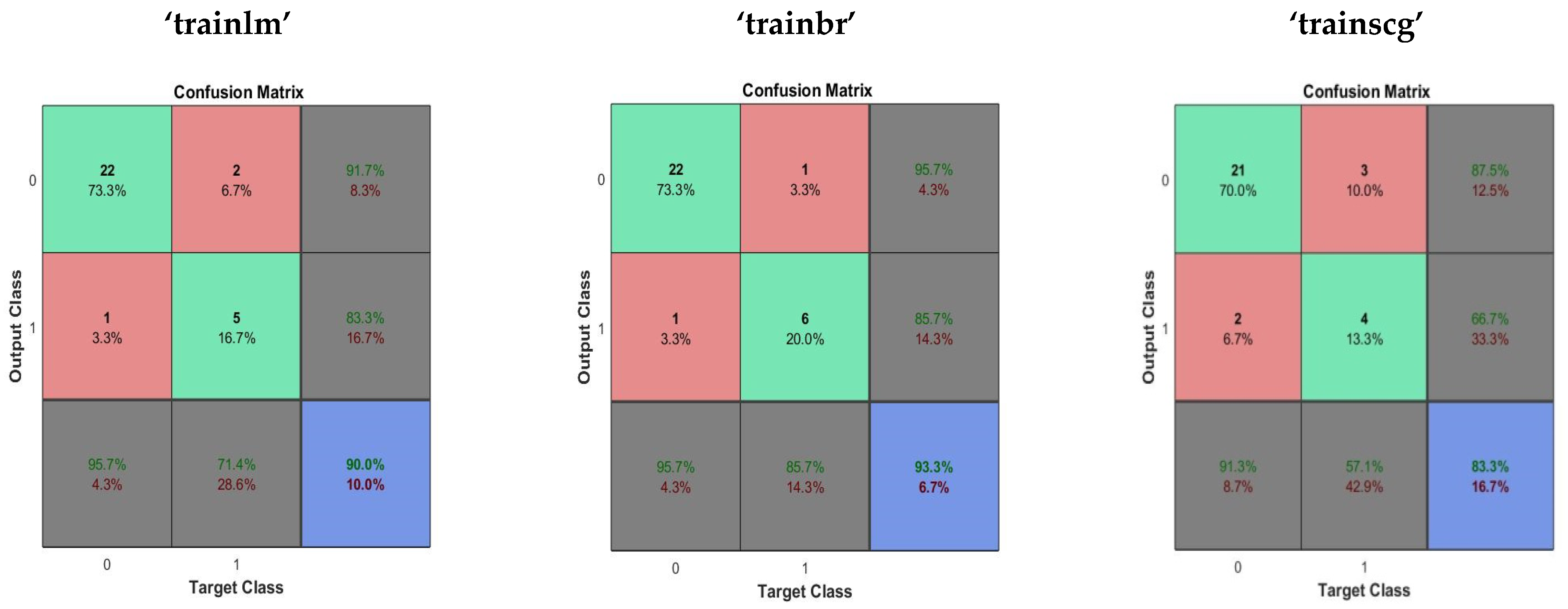
Figure 1. The confusion matrix obtained using the multilayer perceptron with “trainlm”, “trainbr” and “trainscg” training methods.
Computers 10 00031 g001
Figure 2. The confusion matrix obtained for RBF with different levels of spread.
Computers 10 00031 g002
Figure 3. The confusion matrix obtained for GRNN with different levels of spread.
Computers 10 00031 g003
Figure 4. The confusion matrix obtained using the SVM with “linear”, “quadratic” and “rbf” kernels.
Computers 10 00031 g004
Figure 5. The confusion matrix obtained from Random forest using a variety of ensemble methods.
Computers 10 00031 g005
Figure 6. Part-1: Clinical features with predictor importance weights.
Computers 10 00031 g006
Figure 7. Part-2: Clinical features with predictor importance weights.
Computers 10 00031 g007
Figure 8. The 32 selected Clinical features ranked in decreasing order based on their importance in the prediction.
Computers 10 00031 g008
Figure 9. The 20 discarded Clinical features ranked in decreasing order based on their importance in the prediction.
Computers 10 00031 g009
Table 1. The performance evaluation of multilayer perceptron neural network.
Training AlgorithmPerformance Measures
AccuracySensitivitySpecificityPrecisionF_ScoreG-Mean
“trainlcg”0.84990.62200.96430.88890.72850.7740
“trainslm”0.87500.73410.92960.80900.76910.8257
“trainbr”0.90830.79760.97810.93300.84760.8791
Table 2. The performance evaluation of RBF.
SpreadPerformance Measures
AccuracySensitivitySpecificityPrecisionF_ScoreG-Mean
Spread “Normal”0.76660.40470.95650.66670.40000.5228
Spread “Small”0.76670.47610.85920.60610.52100.6177
Spread “Large”0.81660.83330.81570.62270.71170.8225
Table 3. The performance evaluation of the General Regression Neural Network (GRNN).
SpreadPerformance Measures
AccuracySensitivitySpecificityPrecisionF_ScoreG-Mean
Spread “Normal”0.81670.54760.88090.94440.48810.5630
Spread “Small”0.83330.46820.97820.91660.56640.6489
Spread “Large”0.78330.40470.88090.97220.30680.4247
Table 4. The performance evaluation of the Support Vector Machine (SVM).
KernelsPerformance Measures
AccuracySensitivitySpecificityPrecisionF_ScoreG-Mean
“linear”0.84000.56070.93750.77140.63210.7177
“polynomial”0.86670.69640.92750.80470.69450.7841
“rbf”0.80000.4017 0.93280. 67500.50350.6120
Table 5. The performance evaluation of the Random forest.
Ensemble MethodsPerformance Measures
AccuracySensitivitySpecificityPrecisionF_ScoreG-Mean
“LPBoost”0.90330.78570.94560.83030.80120.8607
“GentleBoost”0.90830.67850.97820.90830.77560.8140
“AdaBoostM1”0.90000.67850.96730.87860.76190.8093
“RobustBoost”0.87500.67850.93470.78120.72110.7956
“TotalBoost”0.86660.64280.93450.75350.69130.7740
“RUSBoost”0.86670.75000.90210.69790.72050.8199
“Bag”0.86660.52380.97100.85000.64640.7118
Publisher’s Note: MDPI stays neutral with regard to jurisdictional claims in published maps and institutional affiliations.