
Recommendation Algorithm Using Clustering-Based UPCSim (CB-UPCSim)


Abstract
:1. Introduction
2. Related Work
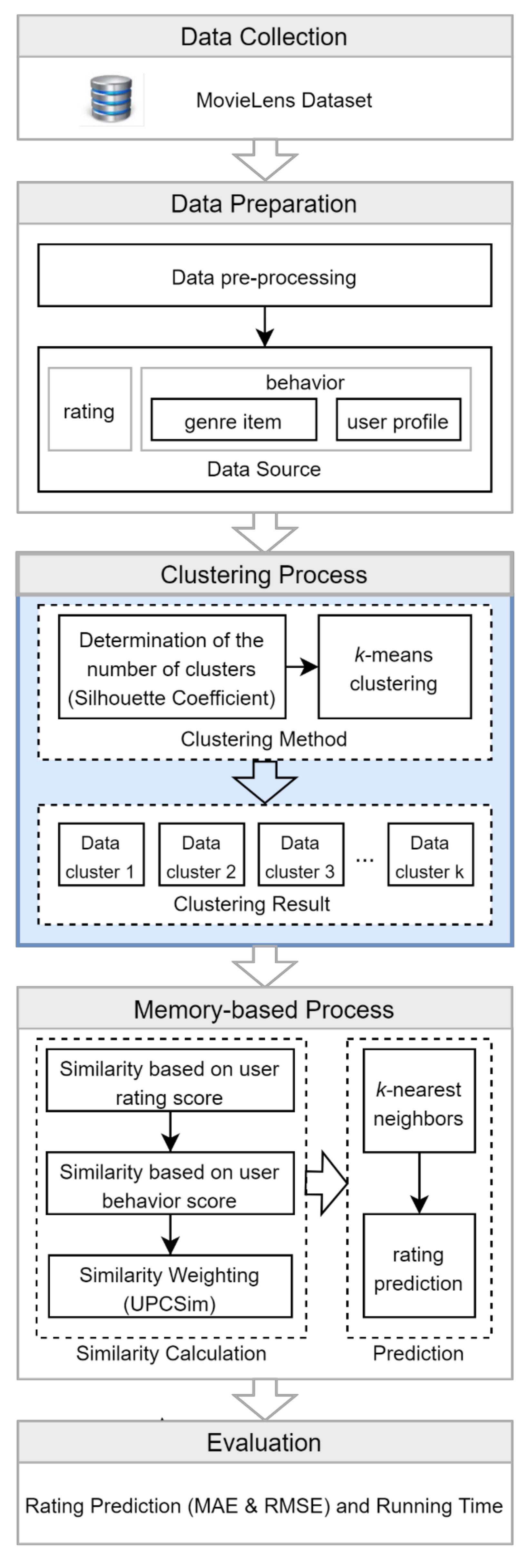
3. Research Method
3.1. Data Collection
3.2. Data Preparation
3.3. Clustering Process
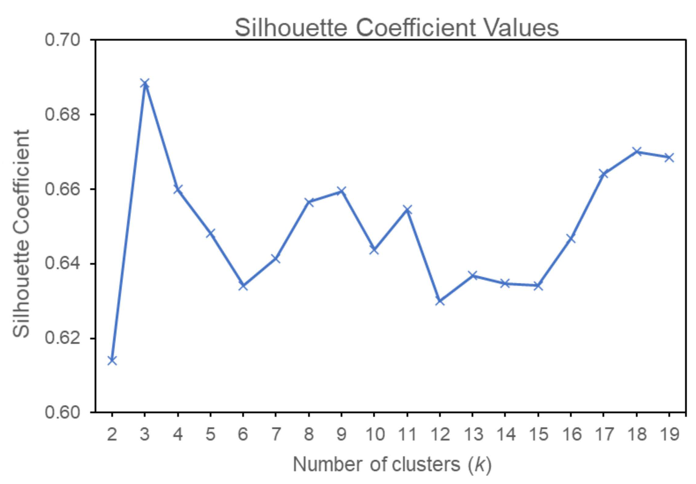
3.3.1. Determination of the Number of Clusters
- Calculate the average distance from one document to another in a cluster using the formula defined in Equation (1).is another document in one cluster , and is the distance between document and document .
- Calculate the average distance from the document to all documents in other clusters, using the formula defined in Equation (2). Then, find the minimum average distance using Equation (3).
- Calculate the Silhouette Coefficient value using Equation (4).
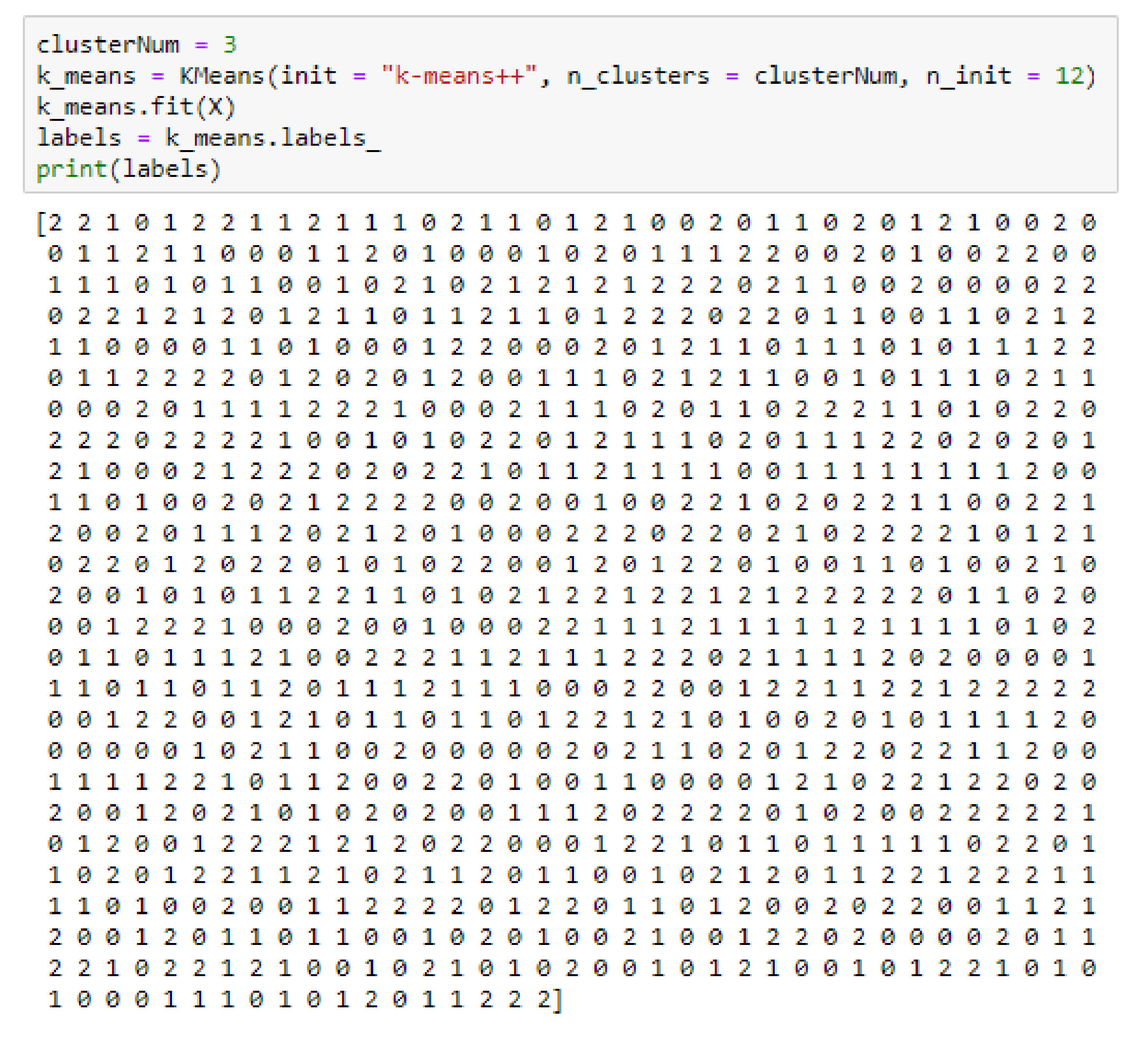
3.3.2. Data Clustering
3.4. Memory-Based Process
3.5. Evaluation
4. Experiment Result and Discussion
4.1. Result of Silhouette Coefficient
4.2. Result of k-Means Clustering
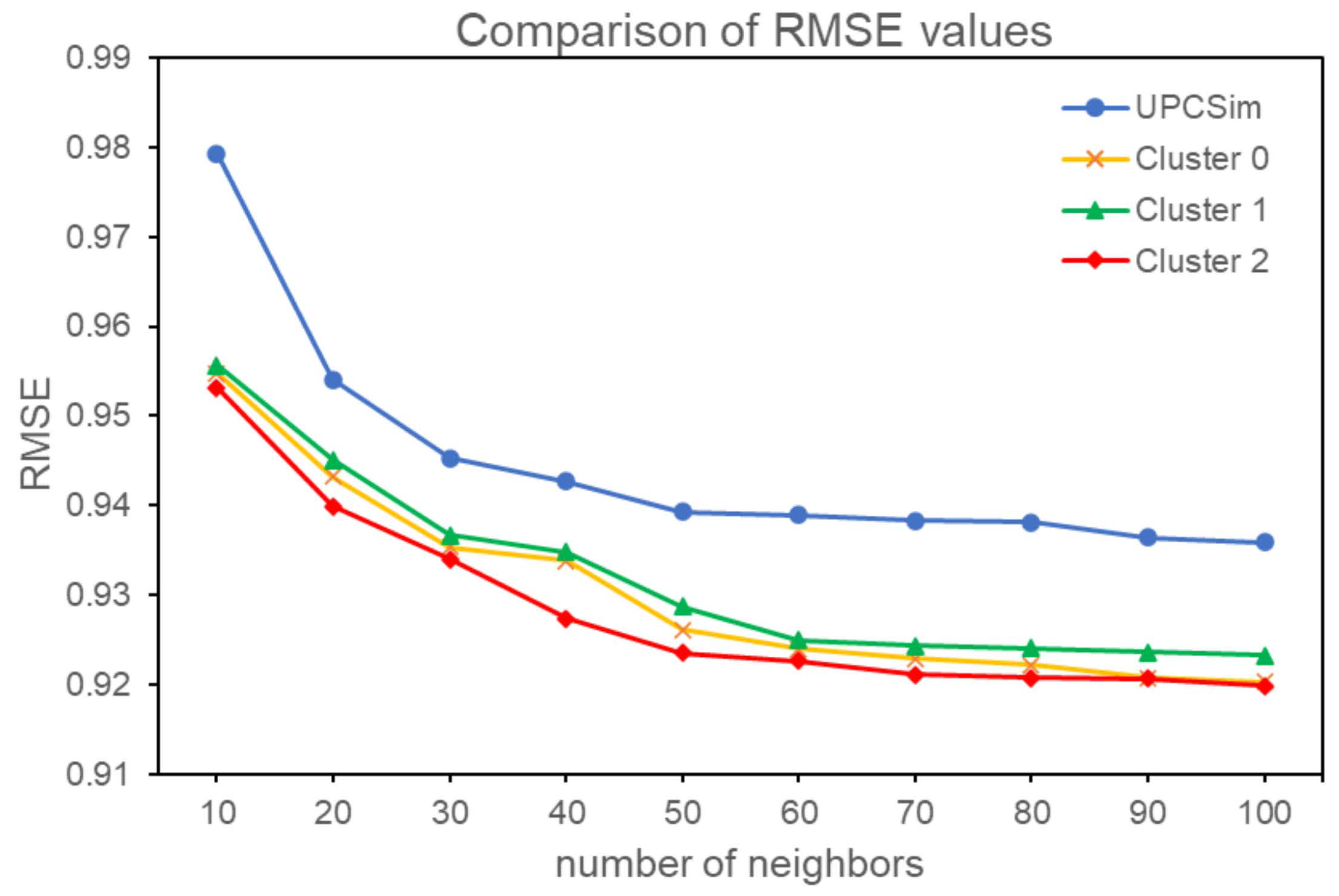
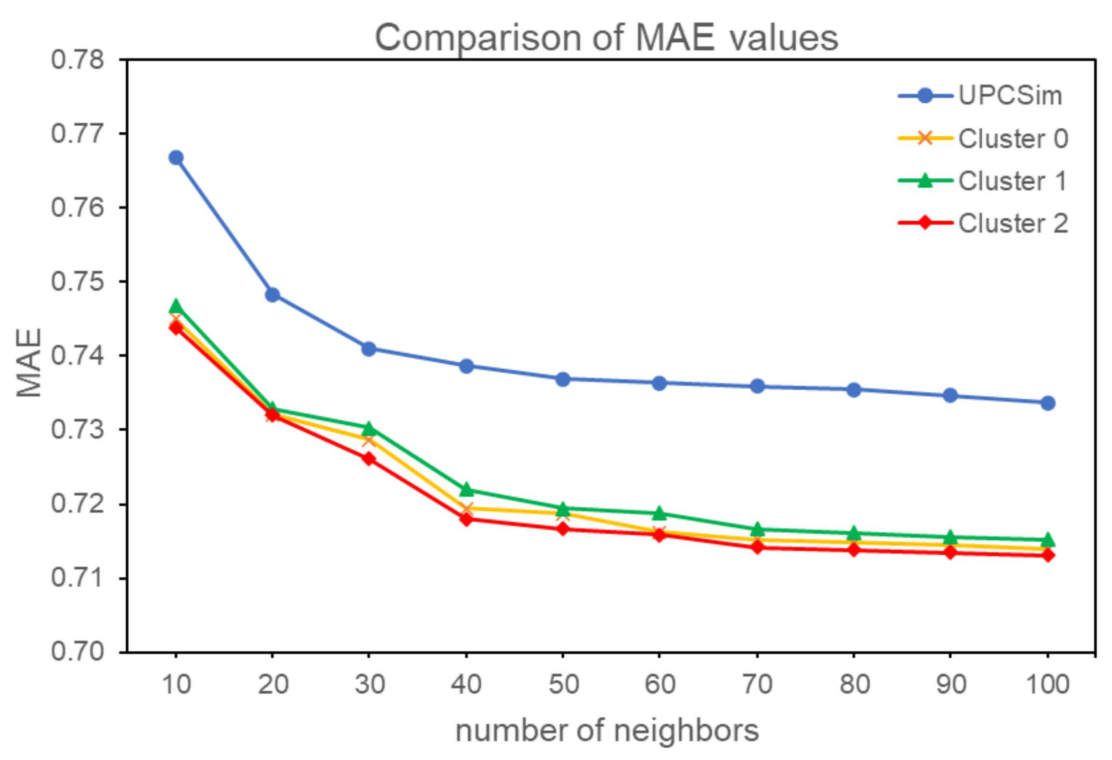
4.3. Result of MAE and RMSE
4.4. Result of Running Time
4.5. Discussion
5. Conclusions
Author Contributions
Funding
Institutional Review Board Statement
Informed Consent Statement
Data Availability Statement
Conflicts of Interest
References
- Kherad, M.; Bidgoly, A.J. Recommendation system using a deep learning and graph analysis approach. arXiv 2020, arXiv:2004.08100. [Google Scholar]
- Sejwal, V.K.; Abulaish, M. Jahiruddin Crecsys: A context-based recommender system using collaborative filtering and lod. IEEE Access 2020, 8, 158432–158448. [Google Scholar] [CrossRef]
- Feng, J.; Fengs, X.; Zhang, N.; Peng, J. An improved collaborative filtering method based on similarity. PLoS ONE 2018, 13, 1–18. [Google Scholar] [CrossRef] [PubMed]
- Su, Z.; Lin, Z.; Ai, J.; Li, H. Rating Prediction in Recommender Systems based on User Behavior Probability and Complex Network Modeling. IEEE Access 2021, 9, 30739–30749. [Google Scholar] [CrossRef]
- Sardianos, C.; Papadatos, G.B.; Varlamis, I. Optimizing parallel collaborative filtering approaches for improving recommendation systems performance. Information 2019, 10, 155. [Google Scholar] [CrossRef] [Green Version]
- Ortega, F.; Mayor, J.; López-Fernández, D.; Lara-Cabrera, R. CF4J 2.0: Adapting Collaborative Filtering for Java to new challenges of collaborative filtering based recommender systems. Knowl.-Based Syst. 2020, 215, 106629. [Google Scholar] [CrossRef]
- Zhang, F.; Qi, S.; Liu, Q.; Mao, M.; Zeng, A. Alleviating the data sparsity problem of recommender systems by clustering nodes in bipartite networks. Expert Syst. Appl. 2020, 149, 113346. [Google Scholar] [CrossRef]
- Alhijawi, B.; Al-Naymat, G.; Obeid, N.; Awajan, A. Novel predictive model to improve the accuracy of collaborative filtering recommender systems. Inf. Syst. 2021, 96, 101670. [Google Scholar] [CrossRef]
- Wang, D.; Yih, Y.; Ventresca, M. Improving neighbor-based collaborative filtering by using a hybrid similarity measurement. Expert Syst. Appl. 2020, 160, 113651. [Google Scholar] [CrossRef]
- Liu, H.; Hu, Z.; Mian, A.; Tian, H.; Zhu, X. A new user similarity model to improve the accuracy of collaborative filtering. Knowl.-Based Syst. 2014, 56, 156–166. [Google Scholar] [CrossRef] [Green Version]
- Patra, B.K.; Launonen, R.; Ollikainen, V.; Nandi, S. A new similarity measure using Bhattacharyya coefficient for collaborative filtering in sparse data. Knowl.-Based Syst. 2015, 82, 163–177. [Google Scholar] [CrossRef]
- Polatidis, N.; Georgiadis, C.K. A multi-level collaborative filtering method that improves recommendations. Expert Syst. Appl. 2016, 48, 100–110. [Google Scholar] [CrossRef] [Green Version]
- Zhang, F.; Zhou, W.; Sun, L.; Lin, X.; Liu, H.; He, Z. Improvement of Pearson similarity coefficient based on item frequency. Int. Conf. Wavelet Anal. Pattern Recognit. 2017, 1, 248–253. [Google Scholar] [CrossRef]
- Sun, S.B.; Zhang, Z.H.; Dong, X.L.; Zhang, H.R.; Li, T.J.; Zhang, L.; Min, F. Integrating triangle and jaccard similarities for recommendation. PLoS ONE 2017, 12, e183570. [Google Scholar] [CrossRef] [PubMed] [Green Version]
- Wu, C.; Wu, J.; Luo, C.; Wu, Q.; Liu, C.; Wu, Y.; Yang, F. Recommendation algorithm based on user score probability and project type. Eurasip J. Wirel. Commun. Netw. 2019, 2019, 80. [Google Scholar] [CrossRef]
- Widiyaningtyas, T.; Hidayah, I.; Adji, T.B. User profile correlation-based similarity (UPCSim) algorithm in movie recommendation system. J. Big Data 2021, 8, 52. [Google Scholar] [CrossRef]
- Lestari, S.; Adji, T.B.; Permanasari, A.E. WP-Rank: Rank Aggregation based Collaborative Filtering Method in Recommender System. Int. J. Eng. Technol. 2018, 7, 193–197. [Google Scholar]
- Tran, C.; Kim, J.Y.; Shin, W.Y.; Kim, S.W. Clustering-Based Collaborative Filtering Using an Incentivized/Penalized User Model. IEEE Access 2019, 7, 62115–62125. [Google Scholar] [CrossRef]
- Vellaichamy, V.; Kalimuthu, V. Hybrid collaborative movie recommender system using clustering and bat optimization. Int. J. Intell. Eng. Syst. 2017, 10, 38–47. [Google Scholar] [CrossRef]
- Yu, P. Collaborative filtering recommendation algorithm based on both user and item. In Proceedings of the 2015 4th International Conference on Computer Science and Network Technology (ICCSNT), Harbin, China, 19–20 December 2015; pp. 239–243. [Google Scholar] [CrossRef]
- Jiawei, H.; Micheline, K.; Jian, P. Data Mining: Concepts and Techniques Preface and Introduction; Elsevier: New York, NY, USA, 2012; ISBN 9780123814791. [Google Scholar]
- Harper, F.M.; Konstan, J.A. The movielens datasets: History and context. ACM Trans. Interact. Intell. Syst. 2015, 5, 1–19. [Google Scholar] [CrossRef]
- Aggarwal, C.; Reddy, C. Data Clustering: Algorithms and Applications; Taylor & Francis Group, LLC.: Abingdon, UK, 2014; ISBN 9781466558229. [Google Scholar]
- Garg, T.; Malik, A. Survey on Various Enhanced K-Means Algorithms. Int. J. Adv. Res. Comput. Commun. Eng. 2014, 3, 8525–8527. [Google Scholar] [CrossRef]
- Indhu, R.; Porkodi, R. Comparison of Clustering Algorithm. Int. J. Sci. Res. Comput. Sci. Eng. Inf. Technol. 2018, 3, 218–223. [Google Scholar]
- Awawdeh, S.; Edinat, A.; Sleit, A. An Enhanced K-Means Clustering Algorithm for Multi-Attributes Data. Int. J. Comput. Sci. Inf. Secur. 2019, 17. Available online: https://scholar.google.com/scholar?hl=en&as_sdt=0%2C5&q=An+Enhanced+K-means+Clustering+Algorithm+for+Multi-+attributes+Data&btnG= (accessed on 14 April 2021).
- Zaki, M.J.; Meira, W. Data Mining and Analysis: Fundamental Concepts and Algorithms; Cambridge University Press: New York, NY, USA, 2014. [Google Scholar]
- Ulian, D.Z.; Becker, J.L.; Marcolin, C.B.; Scornavacca, E. Exploring the effects of different Clustering Methods on a News Recommender System. Expert Syst. Appl. 2021, 183, 115341. [Google Scholar] [CrossRef]
- Raval, U.R.; Jani, C. Implementing & Improvisation of K-Means Clustering Algorithm. Int. J. Comput. Sci. Mob. Comput. 2016, 55, 191–203. Available online: http://www.ijcsmc.com/docs/papers/May2016/V5I5201647.pdf (accessed on 14 April 2021).
- Jose, J.T.; Zachariah, U.; Lijo, V.P.; Gnanasigamani, L.J.; Mathew, J. Case study on enhanced K-means algorithm for bioinformatics data clustering. Int. J. Appl. Eng. Res. 2017, 12, 15147–15151. [Google Scholar]
- Bangoria Bhoomi, M. Enhanced K-Means Clustring Algorithm To Reduce Time Complexity for Numeric Values. Int. J. Adv. Eng. Res. Dev. 2014, 5, 876–879. [Google Scholar] [CrossRef]
- Zhang, F.; Gong, T.; Lee, V.E.; Zhao, G.; Rong, C.; Qu, G. Fast algorithms to evaluate collaborative filtering recommender systems. Knowl.-Based Syst. 2016, 96, 96–103. [Google Scholar] [CrossRef]
- Zheng, M.; Min, F.; Zhang, H.R.; Chen, W. Bin Fast Recommendations with the M-Distance. IEEE Access 2016, 4, 1464–1468. [Google Scholar] [CrossRef]
- Fan, X.; Chen, Z.; Zhu, L.; Liao, Z.; Fu, B. A Novel Hybrid Similarity Calculation Model. Sci. Program. 2017, 2017, 4379141. [Google Scholar] [CrossRef] [Green Version]
- Kuhn, M.; Johnson, K. Applied Predictive Modeling; Springer: New York, NY, USA, 2013; ISBN 9781461468493. [Google Scholar]
- Nguyen, L.V.; Hong, M.S.; Jung, J.J.; Sohn, B.S. Cognitive similarity-based collaborative filtering recommendation system. Appl. Sci. 2020, 10, 4183. [Google Scholar] [CrossRef]
- Nguyen, L.V.; Nguyen, T.H.; Jung, J.J.; Camacho, D. Extending collaborative filtering recommendation using word embedding: A hybrid approach. Concurr. Comput. 2021, e6232. [Google Scholar] [CrossRef]
- Logesh, R.; Subramaniyaswamy, V.; Malathi, D.; Sivaramakrishnan, N.; Vijayakumar, V. Enhancing recommendation stability of collaborative filtering recommender system through bio-inspired clustering ensemble method. Neural Comput. Appl. 2020, 32, 2141–2164. [Google Scholar] [CrossRef]


| Product | Product Type | |||||||
|---|---|---|---|---|---|---|---|---|
| G1 | G2 | G3 | G4 | G5 | G6 | G7 | G8 | |
| p1 | 0 | 1 | 1 | 1 | 0 | 0 | 0 | 0 |
| p2 | 1 | 0 | 0 | 1 | 0 | 1 | 0 | 0 |
| p3 | 0 | 0 | 0 | 0 | 0 | 1 | 1 | 0 |
| p4 | 0 | 0 | 0 | 0 | 0 | 1 | 0 | 0 |
| p5 | 0 | 0 | 0 | 0 | 1 | 0 | 0 | 1 |
| p6 | 0 | 0 | 0 | 0 | 1 | 0 | 0 | 1 |
| p7 | 0 | 0 | 0 | 1 | 0 | 0 | 0 | 0 |
| Data | Before Clustering | After Clustering | ||
|---|---|---|---|---|
| Cluster 0 | Cluster 1 | Cluster 2 | ||
| #users | 943 | 319 | 336 | 288 |
| #ratings | 100,000 | 32,906 | 34,370 | 32,724 |
| % users | 100% | 33.83% | 35.63% | 30.54% |
| % ratings | 100% | 32.91% | 34.37% | 32.72% |
| sparsity of ratings | 93.70% | 93.87% | 93.92% | 93.24% |
| density of ratings | 6.30% | 6.13% | 6.08% | 6.76% |
| N | MAE | |||
|---|---|---|---|---|
| Before Clustering | After Clustering | |||
| UPCSim | Cluster 0 | Cluster 1 | Cluster 2 | |
| 10 | 0.7669 | 0.7450 | 0.7469 | 0.7439 |
| 20 | 0.7483 | 0.7321 | 0.7329 | 0.7320 |
| 30 | 0.7410 | 0.7287 | 0.7303 | 0.7261 |
| 40 | 0.7387 | 0.7194 | 0.7220 | 0.7180 |
| 50 | 0.7369 | 0.7187 | 0.7194 | 0.7167 |
| 60 | 0.7364 | 0.7162 | 0.7188 | 0.7159 |
| 70 | 0.7359 | 0.7152 | 0.7167 | 0.7142 |
| 80 | 0.7355 | 0.7148 | 0.7161 | 0.7138 |
| 90 | 0.7347 | 0.7145 | 0.7156 | 0.7135 |
| 100 | 0.7337 | 0.7139 | 0.7152 | 0.7131 |
| Average | 0.7408 | 0.7219 | 0.7234 | 0.7207 |
| N | RMSE | |||
|---|---|---|---|---|
| Before Clustering | After Clustering | |||
| UPCSim | Cluster 0 | Cluster 1 | Cluster 2 | |
| 10 | 0.9793 | 0.9548 | 0.9557 | 0.9532 |
| 20 | 0.9541 | 0.9432 | 0.9451 | 0.9399 |
| 30 | 0.9453 | 0.9354 | 0.9367 | 0.9340 |
| 40 | 0.9427 | 0.9338 | 0.9348 | 0.9274 |
| 50 | 0.9393 | 0.9261 | 0.9287 | 0.9235 |
| 60 | 0.9389 | 0.9240 | 0.9250 | 0.9226 |
| 70 | 0.9383 | 0.9229 | 0.9243 | 0.9211 |
| 80 | 0.9381 | 0.9222 | 0.9241 | 0.9208 |
| 90 | 0.9364 | 0.9208 | 0.9236 | 0.9207 |
| 100 | 0.9359 | 0.9203 | 0.9233 | 0.9199 |
| Average | 0.9448 | 0.9304 | 0.9321 | 0.9283 |
| N | Running Time (Seconds) | |||
|---|---|---|---|---|
| Before Clustering | After Clustering | |||
| UPCSim | Cluster 0 | Cluster 1 | Cluster 2 | |
| 10 | 4.78 | 0.70 | 0.75 | 0.67 |
| 20 | 4.82 | 0.81 | 0.85 | 0.75 |
| 30 | 5.02 | 0.91 | 0.89 | 0.81 |
| 40 | 5.27 | 0.89 | 0.95 | 0.86 |
| 50 | 5.68 | 0.96 | 0.98 | 0.89 |
| 60 | 5.99 | 0.98 | 1.00 | 0.87 |
| 70 | 6.02 | 0.99 | 1.01 | 0.90 |
| 80 | 6.10 | 1.01 | 1.03 | 0.92 |
| 90 | 6.15 | 1.03 | 1.02 | 0.94 |
| 100 | 6.28 | 1.07 | 1.06 | 0.94 |
| Average | 5.61 | 0.94 | 0.95 | 0.86 |
Publisher’s Note: MDPI stays neutral with regard to jurisdictional claims in published maps and institutional affiliations. |
© 2021 by the authors. Licensee MDPI, Basel, Switzerland. This article is an open access article distributed under the terms and conditions of the Creative Commons Attribution (CC BY) license (https://creativecommons.org/licenses/by/4.0/).
Share and Cite
Widiyaningtyas, T.; Hidayah, I.; Adji, T.B. Recommendation Algorithm Using Clustering-Based UPCSim (CB-UPCSim). Computers 2021, 10, 123. https://doi.org/10.3390/computers10100123
Widiyaningtyas T, Hidayah I, Adji TB. Recommendation Algorithm Using Clustering-Based UPCSim (CB-UPCSim). Computers. 2021; 10(10):123. https://doi.org/10.3390/computers10100123
Chicago/Turabian StyleWidiyaningtyas, Triyanna, Indriana Hidayah, and Teguh Bharata Adji. 2021. "Recommendation Algorithm Using Clustering-Based UPCSim (CB-UPCSim)" Computers 10, no. 10: 123. https://doi.org/10.3390/computers10100123
APA StyleWidiyaningtyas, T., Hidayah, I., & Adji, T. B. (2021). Recommendation Algorithm Using Clustering-Based UPCSim (CB-UPCSim). Computers, 10(10), 123. https://doi.org/10.3390/computers10100123