Analytical and Numerical Evaluation of Co-Scheduling Strategies and Their Application

Abstract

Applications in high-performance computing (HPC) may not use all available computational resources, leaving some of them underutilized. By co-scheduling, i.e., running more than one application on the same computational node, it is possible to improve resource utilization and overall throughput. Some applications may have conflicting requirements on resources and co-scheduling may cause performance degradation, so it is important to take it into account in scheduling decisions. In this paper, we formalize the co-scheduling problem and propose multiple scheduling strategies to solve it: an optimal strategy, an online strategy and heuristic strategies. These strategies vary in terms of the optimality of the solution they produce and a priori information about the system they require. We show theoretically that the online strategy provides schedules with a competitive ratio that has a constant upper limit. This allows us to solve the co-scheduling problem using heuristic strategies that approximate this online strategy. Numerical simulations show how heuristic strategies compare to the optimal strategy for different input systems. We propose a method for measuring input parameters of the model in practice and evaluate this method on HPC benchmark applications. We show the high accuracy of the measurement method, which allows us to apply the proposed scheduling strategies in the scheduler implementation.

1. Introduction

A number of scientific fields rely on high-performance computing (HPC) for running simulations and data analysis applications. For example, ref. [1] reviews the deployment of quantum chemistry methods on HPC platforms, ref. [2] describes flood simulation applications in the civil engineering field running on HPC architectures, and [3] considers the scheduling problem for cybersecurity applications. Scheduling plays a critical role in HPC systems, as HPC schedulers are a primary interface between users and computational resources. They ensure the minimal queue wait time, fairness of resource allocation and high resource utilization. In addition to this, with growing scales of computational clusters, they must ensure a low power consumption [4], a low computational cost [5] when they are deployed in cloud, and support for complex scientific workflows [6].

Commonly used batch schedulers in HPC, for example, SLURM [7] or SGE [8], work by computing a schedule as a sequence of reservations of cluster resources to each task for a given amount of time. The parameters of each task (time duration, number of nodes, amount of memory) are provided by the user during task submission. When execution of the task reaches the time limit, the task is terminated, so the user has to resubmit the task with a longer time duration. Due to this, users very often over-estimate time requirements. For example, the survey in [9] reports that 69% of submitted tasks use less than 25% of their requested time. Although scheduling algorithms can be adapted to account for over-estimated time [10], the problem of over-estimation of other resources still remains. The same survey reports that only 31% of tasks use more than 75% of the requested memory.

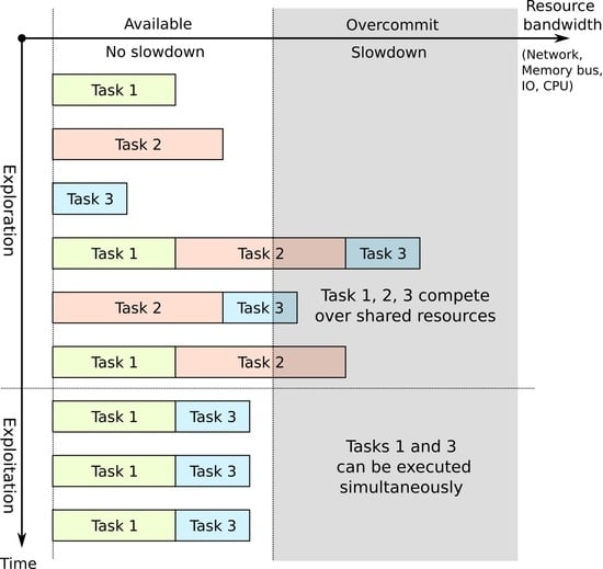
An alternative approach to reservation-based scheduling, called co-scheduling, has started to appear recently in the scientific literature. The idea behind this approach is that multiple tasks may be scheduled to run simultaneously on the same computational node, when they do not interfere with each other. This allows one to increase cluster utilization and overall task throughput (e.g., [11,12,13]). Each cluster node has multiple different resources that are rarely fully utilized at the same time by a single application. Such resources may include memory cache size, memory bus bandwidth, network bandwidth, computational units in CPU, accelerator cards, etc. Usually, applications reach maximum utilization (a bottleneck) on one of these resources, which limits the use of other resources. Additionally, resource utilization can be controlled by the scheduler using technologies such as cache partitioning [14] or voltage scaling [15]. Applications that have bottlenecks on different resources can be potentially scheduled together as they would not interfere with each other.

Deciding which tasks can be executed simultaneously with minimal interference in advance requires the model of task performance degradation. In practice, this model is not easy to obtain, as it can only be estimated from the experiments. In addition to this, it must be reproducible when task behaviour changes due to different factors, such as different input parameters and hardware configurations, or it may even change randomly when the task is running non-deterministic algorithms. Instead, due to these limitations, in this paper we approach this problem as an online scheduling problem, where scheduling decisions are made dynamically based on the observed information about each task performance. We propose a method of measuring task processing speed in for the runtime that can be used for providing a feedback value to the scheduler.

To show the feasibility of the proposed approach, we have formalized the co-scheduling problem in terms of the scheduling theory. We have considered deterministic and stochastic problem definitions and proposed several scheduling strategies, including the optimal strategy, that can be used to solve the problem. These strategies vary in terms of the optimality of the solution they produce and in terms of the information about each task that is available to them. We have compared each strategy with the optimal strategy by deriving the analytics bound on the competitive ratio for an online strategy and by estimating it using numerical simulations for non-deterministic strategies.

The main contributions of this paper are summarized as follows:

1.

We have formalized the deterministic co-scheduling problem in terms of scheduling theory and proposed the optimal strategy and an online strategy (referred to as FCS) to solve it. We have analytically derived an upper boundary limit for the competitive ratio of the FCS strategy.

2.

We have formalized the stochastic co-scheduling problem and proposed search-based strategies for solving it. Using numerical simulations, we have shown how competitive ratios of these strategies are affected by applications and the changes in task processing speed.

3.

We have proposed a method of measuring task processing speed in the runtime. Using benchmarks that mimic HPC applications, we have shown a high accuracy of the method in different co-scheduling environments.

The rest of the paper is organized as follows. First, in Section 2, we give an overview of the existing work related to co-scheduling. Section 3 defines a taxonomy of scheduling problems and formalizes a deterministic co-scheduling problem. In Section 4, we present optimal and online strategies and their comparison for this problem. In Section 5, we formalize a stochastic co-scheduling problem and present strategies for solving it. In Section 6, we propose a method for measuring task processing speed and experimentally show its accuracy. In Section 8, we describe experiments with numerical simulations and present their results. Finally, Section 9 and Section 10 provide practical considerations about strategy implementation and brief concluding remarks.

2. Related Work

The problem of scheduling computational tasks on shared resources has started to appear recently in the scientific literature in the HPC field. For example, there are workshop proceeding papers [16] dedicated to the co-scheduling problem of HPC applications. These particular papers, along with others, are mostly focused on the feasibility of this approach in general and providing proof of concept implementations. In [17], the authors showed that by sharing nodes between two distributed applications instead of running these applications on dedicated nodes may improve performance by 20% in terms of both execution time and system throughput. In [11], this approach is referred to as job striping and it was shown to produce a more than 22% increase in system throughput in benchmark and real applications. In [12], the authors presented scheduler implementation that applied the co-scheduling strategy and reported an up 35% increase in throughput. The papers [13,18] report makespan decreases of up to 26% and 55% correspondingly due to the co-scheduling of two applications. In our work, however, we focus mostly on the theoretical part of the co-scheduling problem. For example, in our previous paper [19], we have showed how makespan may decrease due to co-scheduling as a function of application slowdown.

There are also theoretical publications focused on modeling the co-scheduling problem. Some authors in their publications approach it as an offline scheduling problem, where all task data are available at the start and an optimal schedule can be constructed in advance. Among these publications are [14,20,21], where the authors solve the offline scheduling problem with resource constraint. They model the CPU cache partition size as a controllable task resource and define task speedup as a function of the cache partition size. These speedup functions are assumed to be known in advance and they are used for constructing an optimal schedule.

The problem of measuring task speedup profiles that can later be used for offline scheduling is described, for example, in [18,22]. In the first paper, the authors used a machine learning approach for constructing a model of application slowdown as a function of CPU performance counters values. The training dataset was obtained by measuring performance counters and execution times of applications in ideal conditions and in pairs with other applications. The authors fitted different models on the training data from 27 benchmark applications and reported that the best model (random forest) provided an 80% prediction accuracy for unseen applications. The second paper presents a similar approach but with a different machine learning model. The authors fitted a support vector machine model of makespan decrease (a boolean value) as a function of the metrics measuring CPU, memory and IO intensities. The constructed models in both papers were used to decide whether or not tasks from the queue can be co-scheduled (in pairs) on the same cluster nodes.

In this paper, we propose a different approach, where task performance degradation is measured over the runtime and co-scheduling decisions are made dynamically. We consider that the approach of offline scheduling may produce unreliable models, as it cannot account for all factors affecting the application performance, which are important for offline scheduling. First, there may be dependencies on input parameters. Application behaviour may change drastically when it is processing a small dataset that fits into CPU caches compared to a large dataset that does not fit into CPU caches. Second, changes in system configuration may also affect application performance. For example, cluster nodes may share the same interconnect network and applications running on these nodes (separately) may affect each other [23]. Third, tasks may have stochastic resource requirements, for example, when they are running non-deterministic algorithms [10]. In addition to this, online scheduling allows for better controlling co-scheduling, when, for example, only certain parts of applications can be co-scheduled.

The dynamic co-scheduling problem for HPC applications is not covered in the scientific literature to the same extent as offline scheduling and implementation-related problems. Among the available publications there is [15], where the authors propose using a reinforcement learning algorithm for online co-scheduling of services and batch HPC workloads. Computational resources for HPC workloads in the described setup are provided as opportunistic resources when the service meets its target service level agreement (query latency). The authors proposed dynamically scaling the CPU clock frequency of the cores that run HPC workloads based on the values of CPU performance counters and the feedback reported by the service. Using this approach allowed the authors to improve server utilization by up to 70% compared to using dedicated servers for each workload.

A similar online scheduling problem is covered in the context of thread scheduling in simultaneous multithreading (SMT) CPUs. For example, there are [24,25,26], dating back to the year 2000. The general idea, proposed in these papers, is to dynamically measure the instruction per cycle (IPC) values of each thread, when it is running alone on a core and when it is running in parallel with other threads. Then, the ratio of these two values is used for making scheduling decisions. The authors report decreases in the task turnaround time (the sum of queue wait time and execution time) by 17% [24] and 7–15% [25]. In the follow-up paper [27], the authors revisited this approach and showed that although the turnaround time decrease may be high, the instruction throughput gain is smaller than 3%. The authors showed this experimentally by measuring the instruction throughput of each benchmark application thread in all possible combinations with other threads. Then, these values were used to construct an optimal schedule which was compared to a naive strategy of running all threads in parallel in the queue order.

Earlier in our research [19], we applied the same method as in [27] to show how the makespan of a naive strategy of running all tasks simultaneously compares to the optimal strategy. We have showed that the difference between makespan values increases significantly as a function of tasks slowdown. We have also provided theoretical boundaries for the task slowdown value when a naive parallel strategy cannot be applied.

In the literature, there are several approaches for controlling applications to implement co-scheduling. In [14], cache partitioning technology was used for assigning each core a specified amount of an available shared cache. When the application has a bottleneck in cache access, restricting its size allows one to control the application processing speed. In [15], the approach of changing voltage and frequency of individual CPU cores was used. By scaling the frequency of the cores that run the same task, it is possible to change the task processing speed. In [12], the authors used a different approach of migrating applications in virtual machines between nodes. This approach allows one to implement task preemption, so one task that is in conflict with other tasks could be suspended and migrated to a different node. In the papers that propose offline scheduling strategies [18,22], the authors do not control the resource allocation or processing speed of each task in runtime, but instead decide on which task combinations to schedule in advance, before task processing starts.

In this paper, we propose scheduling strategies that rely on task preemption. A preemption interface can be provided at the software level by the operating system scheduler or by a hypervisor. Unlike CPU dynamic voltage control or cache partitioning technologies, preemption does not allow one to control the application execution speed, but as an advantage, it does not require support at the hardware level.

In terms of scheduling strategies, this paper relates to the online scheduling strategies for SMT CPUs in the aforementioned papers. We also propose using similar metrics for measuring task processing speed and we are also relying on task preemption to implement co-scheduling. Unlike thread scheduling, we are focusing on the higher level schedulers (workflow managers or batch schedulers) that work on top of the operating system scheduler. Due to this, we do not meet the requirement of having a very low operational overhead, which allows us to apply more computation-intensive strategies; furthermore, additional information about application runtime is available for making scheduling decisions.

3. The Problem of Task Co-Scheduling

In classical scheduling theory, there are assumptions [28] that may limit its applicability to the co-scheduling problem. At first, each task can be processed by at most one machine and each machine can process at most one task. Second, the task execution time does not change in time. Third, the task execution time is known in advance. In the problem of co-scheduling all of the propositions of classical scheduling theory are changed. That is, a single machine may process more than one task, task processing speed changes due to interference of other tasks and their required amount of work or processing time are unknown. Nevertheless, in this paper, we will abide with conventional scheduling theory notation and methods whenever possible.

In this paper, we will distinguish scheduling models and their strategies as deterministic and stochastic following the notation from [29]. Deterministic scheduling models assume that there is a finite number of tasks and information about each task (e.g., processing time) is represented as an exact quantity. In stochastic scheduling models, information about tasks is not known exactly in advance and represented as random variables. Some parameters of distributions of these random variables may be available before the task starts, but the exact value (its realization) is only known when the task is completed.

Deterministic scheduling models can vary by the availability of the information about each task. When all information about each task is known in advance, such models are referred to as offline and their strategies are called offline strategies. Contrary to offline models, there are online models, where the number of tasks and information about them are unknown in advance. The scheduler becomes aware of the tasks only when they are added to its queue. In the computer science field, a different notation of static and dynamic strategies is commonly used instead of offline and online strategies (for example, in [5]).

Online scheduling models can be further divided as clairvoyant and non-clairvoyant models [29]. Once the task is presented to the scheduler, the information related to the task processing time can either be available, which makes the model clairvoyant, or unknown until task completion, which makes the model non-clairvoyant.

Problem Formulation

In this section, we will formalize the task co-scheduling problem. We will only consider the stationary problem definition, where the number of tasks, their processing speeds in all combinations and required amount of work do not change over time. This assumption limits the scope of theoretical methods that can be used. In practice, it may not always hold, but the results obtained for a stationary system can be useful for time-dependent systems as well.

We will use the following notation to formalize the scheduling problem. There are n tasks (applications) denoted as $T=\{T_1,\dots ,T_n\}$. Each $T_i$ requires $b_i$ work units to be performed before its completion. Any subset of tasks from T can be ran simultaneously on the same machine. We will refer to these subsets as task combinations. There are $m=2^n-1$ possible combinations (subtracting ∅ combination). We denote each combination as $S_j$, $S_j\in 2^T$, where $2^T$ is a set of all subsets of T (power set). $|S_j|$ is the number of tasks in $S_j$.

Tasks are run in combination at their own processing speeds (measured in work unit per time units). Without loss of generality, we consider the speed of the task, when it was running in ideal conditions (in the $S_j=\left\{T_i\right\}$ combination), to be equal to 1. Otherwise, we can divide the required task units of work ($b_i$) by this speed. We denote $a_{i,j}$ as a speedup (or acceleration) of the task $T_i$ in combination $S_j$ compared to ideal conditions. Due to this assumption, we will refer to $a_{i,j}$ as speedup and speed interchangeably (except for the sections related to experiments, where the difference between two terms matters).

Even though task speed cannot increase when it is run in combination with other tasks compared to ideal conditions, hence values $a_{i,j}\le 1$, we will still refer to these values as speedup values. This fact can be generalized into a constraint on values $a_{i,j}$, i.e., that the task speed decreases with the increase in the number of tasks in combination:

$$a_{i,p}\le a_{i,q},\forall (p,q)\mid S_p\subset S_q,i=1,\dots ,n$$

(1)

When $T_i\notin S_j$, then $a_{i,j}=0$, and when $T_i\in S_j$, then $0\le a_{i,j}\le 1$. All values of $a_{i,j}$ form a matrix A with dimensions n by m. We will define the speed of a whole combination as a sum of all task speeds in the combination ($a_j={\sum }_{i=1}^n{a}_{i,j}$).

For the simplicity of the model definition, we assumed that all task combinations are feasible and all are tasks run in a single-node environment. These assumptions do not limit a general case, as task processing speed in combinations containing unfeasible subsets of tasks can be set to zero. Environments with multiple nodes can be modeled as a single-node environment containing combined resources of multiple nodes, without affecting the introduced model definition.

We define a schedule as a sequence of pairs of task combinations and their time interval lengths. We denote a pair at the position k in a schedule as $(S_{j_k},x_{j_k})$, where $x_{j_k}$ is the amount of time the combination $S_{j_k}$ is supposed to run until the scheduler switches to the next pair at the position $k+1$. The index $j_k$ refers to a subsequence of combination indices j, i.e., $j_k\in \{1,\dots ,m\}$ and $k=1,\dots ,K$, where K is the number of pairs in the schedule. We will call this sequence of pairs a feasible schedule when each task completes its required amount of work exactly, i.e., ${\sum }_{k=1}^K{a}_{i,j_k}{x}_{j_k}=b_i\forall i=1,\dots ,n$.

In this paper, we will use makespan as the objective function for the scheduling problem. We define the makespan of a schedule as the completion time of the last task. It can also be written as a sum of the assigned time interval lengths: $C_{max}={\sum }_{k=1}^K{x}_{j_k}$. Since it is a sum, we can reorder its terms and group together the terms corresponding to the same combination and write it as:

$$C_{max}=\sum _{j=1}^m{x}_j,\mathrm{where}{x}_j=\sum _{k\mid j_k=j}{x}_{j_k},j=1,\dots ,m$$

(2)

Now, we consider the problem definition, where preemption is allowed, that is, the scheduler may suspend the execution of tasks from the current combination and continue the execution of other tasks from the next combination. Preemption of combinations may occur even if some of their tasks are not completed; due to this, in a feasible schedule some combinations may be repeated multiple times.

4. Deterministic Co-Scheduling Strategies

In this section, we will cover optimal and online scheduling strategies for solving the co-scheduling problem. The optimal strategy is an offline strategy as it requires all information about tasks to be known at the start. The online strategy that we will consider in this section works under the assumption that the required amount of work is not available to the scheduler at any time point. In the scheduling theory framework, such a strategy would fall into the non-clairvoyant category.

Since the online scheduling strategy works with incomplete information, it may produce sub-optimal solutions. To show the effectiveness of this strategy, we will compare the makespan value that it produces with respect to the optimal makespan value. For this, we will derive the formula for the competitive ratio, i.e., the ratio between these two makespan values. The upper bound of the competitive ratio provides us with an estimation of the worst case. At the end of the section, we will show an example of the worst case, where an upper bound can be reached.

4.1. Optimal Strategy

The problem of finding the schedule with the minimal makespan value can be reduced to finding values of $x_j\ge 0,j=1,\dots ,m$ which have the minimum sum and produce a feasible schedule, i.e., ${\sum }_{j=1}^m{a}_{i,j}{x}_j=b_i\forall i=1,\dots ,n$

This gives us a linear programming problem:

$$\begin{array}{ccc}\mathrm{minimize}\hfill & \sum _{j=1}^m{x}_j\hfill & \\ \mathrm{subject}\mathrm{to}\hfill & Ax=b\hfill & \\ \hfill & x\ge 0\hfill \end{array}$$

(3)

Solving this problem gives us a vector $x^{*}$ of an optimal time distribution between combinations. A schedule can be reconstructed from $x^{*}$ by running each combination $S_j$ for $x_j^{*}$ time (if $x_j^{*}>0$) in any order. In this case, the schedule would be feasible and it will have the minimum makespan. In this paper, we will refer to this strategy as an optimal (OPT) strategy and its makespan value as $C_{max}^{OPT}$.

This optimal strategy is considered an offline strategy, as it requires all information (matrix A and vector b) to be known in advance before running any tasks. Due to this, it cannot be used in practice but can still be used as a reference point for evaluating other strategies.

4.2. Online Strategy

Let us consider the online (non-clairvoyant) formulation of this problem, when the amount of work required for the completion of each task (i.e., vector b) is unknown. The values of matrix A are still known at time 0. To solve this, we propose using an online strategy that always runs in combination with the maximum speed. We will refer to this strategy in the present paper as FCS—Fastest Combination Speed first.

The FCS strategy algorithm is shown in pseudocode in Listing 1. The algorithm iterates until completion of all tasks ($C\ne T$). At each iteration, it searches a combination of active tasks with the maximum sum of the task processing speed. In case there are multiple combinations with the same speed, it will choose the first one in the order of $j=1,\dots ,m$. After such a combination is found, it is run until tbe completion of any of its tasks. In the pseudocode, this step is represented by the function $run\_until\_completion$, which runs the combination and returns a set of tasks that have been completed. After this function is presented, a set of completed tasks is updated and the algorithm proceeds to the next iteration.

Listing 1. Pseudocode for the algorithm of FCS strategy.

4.3. Competitive Ratio of the FCS Strategy

To evaluate the FCS strategy, we will derive an upper bound on its competitive ratio ($\rho$):

$$\rho =\frac{C_{max}^{FCS}}{C_{max}^{OPT}}$$

(4)

The problem of finding an upper bound of $\rho$ boils down to finding values of the matrix A and vector b for which $\rho$ is the maximum value. Matrix A and vector b have constraints on their values as defined in Section 3.

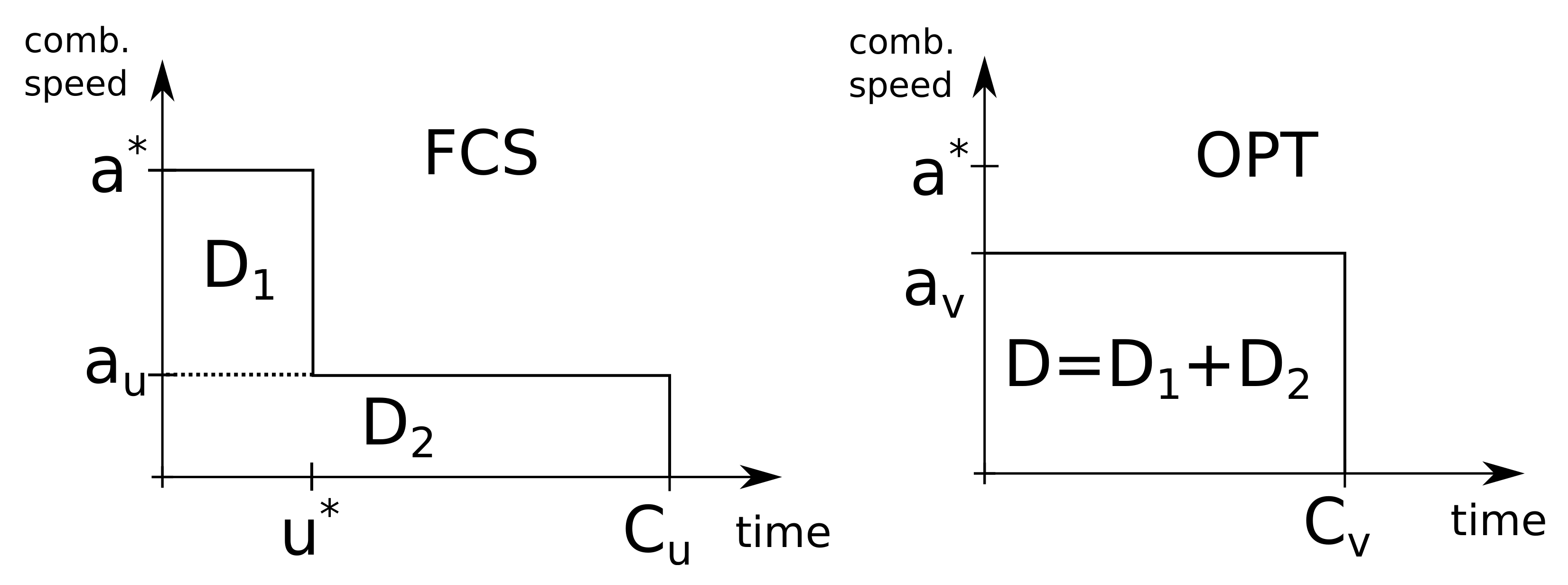
We denote the total amount of work of all tasks as $D={\sum }_{i=1}^n{b}_i$. By combining this with the maximum speed will create the index $j^{*}$ and its speed would be equal to $a^{*}$, i.e., $a_{j^{*}}=a^{*}=ma{x}_{j=1,\dots ,m}{a}_j$. To simplify notation, we will refer to the parameters of the schedule produced by the FCS strategy with u subscript and parameters of the optimal schedule with v subscript, that is, $C_u=C_{max}^{FCS}$ and $C_v=C_{max}^{OPT}$.

In general, the FCS schedule and optimal schedule have forms as shown in Figure 1. Both schedules perform the same amount of work, so the areas under the left and right plots (time multiplied by the processing speed) are the same. The FCS schedule runs in combination with the maximum speed $a^{*}$ until the completion of any of its tasks. We denote the duration of the first combination run as $u^{*}$. After this combination finishes, the schedule proceeds with the remaining combinations of active tasks until all the work is completed. We denote $a_u$ as an average speed of all the remaining combinations until the end of the schedule (at the time point $C_u$), so $a_u\le a^{*}$. Similarly, the optimal schedule runs combinations at the average speed $a_v$, performing D units of the total work until completion at time point $C_v$.

Lemma 1.

Schedules with $a_u=1$ and $a_v=a^{*}$ have the maximum competitive ratio, which is equal to

$$\rho =a^{*}-\frac{u^{*}(a^{*}-1)}{D}$$

(5)

Proof. 

Since both FCS and optimal schedules complete the same amount of work D, we can write

$$D=a^{*}{u}^{*}+(C_u-u^{*})a_u=C_v{a}_v$$

(6)

Then, the competitive ratio can be written as

$$\rho =\frac{C_u}{C_v}=\frac{a_v(D-u^{*}(a^{*}-a_u))}{a_{u}D}$$

(7)

To prove the lemma, we can analyze its derivatives on the variables $a_u$ and $a_v$ that are affected by strategy decisions.

$$\begin{array}{c}\frac{\partial \rho }{\partial a_u}=-\frac{a_v(D-a^{*}{u}^{*})}{D{\left(u^{*}\right)}^2}\\ \frac{\partial \rho }{\partial a_v}=\frac{D-u^{*}(a^{*}-a_u)}{D{a}_u}\end{array}$$

(8)

The feasible region of these values is defined as $1\le a_u\le a^{*}$, $1\le a_v\le a^{*}$. $\frac{\partial \rho }{\partial a_v}$ has no special points within the feasible region (otherwise, $C_u=0$). $\frac{\partial \rho }{\partial a_v}$ has a single feasible special point, which exists only if $D=a^{*}{u}^{*}$, i.e., all of the work is completed in the $j^{*}$ combination. In this case, $\rho$ would take its minimum value ($\rho =1$) as both schedules would be the same.

Within the feasible region, $\frac{d\rho }{d{a}_u}<0$ and $\frac{d\rho }{d{a}_v}>0$. So, the maximum value of $\rho$ is reached at the borders of the region, when $a_u$ has the minimum value (i.e., $a_u=1$) and $a_v$ has the maximum value ($a_v=a^{*}$).

By substituting the values $a_u=1,a_v=a^{*}$ in (7), we can derive the formula (5) for the competitive ratio. □

Function $\rho$ is, in general, an unbounded function, as its derivatives do not have any special points within the feasible region. For example, for a fixed $u^{*}=1$ (which requires $D>1$ to be feasible)m it can become arbitrarily large in the direction of D and $a^{*}$, as its derivatives would be positive.

In the proof of the following theorem, we will consider only the schedules that have the form as defined by the lemma. That is, the optimal strategy runs combinations at the average speed $a^{*}$ and the FCS schedule runs the remaining combinations (after the one $a^{*}$ speed) with an average speed of 1. Along with the feasibility constraints, this form allow us to obtain bounds on the value of D as a function of $a^{*}$. Using these bounds in competitive ratio formula, in turn, will give us its upper bound.

Theorem 1.

Competitive ratio of the FCS strategy is at most 2.

Proof. 

To find the upper bound on $\rho$, we will only consider the schedules with $a_u=1$, $a_v=a^{*}$, as shown by the lemma.

We denote the index of the first combination of the FCS schedule as $j^{*}$, and let us assume without loss of generality that first $k>0$ tasks finish in the $S_{j^{*}}$ combination, i.e.,

$$u^{*}=\frac{b_1}{a_{1,j^{*}}}=\cdots =\frac{b_k}{a_{k,j^{*}}}$$

(9)

The remaining tasks $T_{k+1},\dots ,T_n$ run until completion in FCS in combination with the speed $a_u=1$. As FCS at every iteration selects combinations with the largest speed, any combination of $T_{k+1},\dots ,T_n$ (including the ones that were not selected by FCS) would have a speed no greater than 1; otherwise, they would be selected by FCS and then $a_u>1$. So, we can write that

$$a_j=\sum _{i=1}^n{a}_{i,j}=\sum _{i=k+1}^n{a}_{i,j}=1,\forall j\mid S_j\in 2^{\{T_{k+1},\dots ,T_n\}}$$

(10)

Consider $v={(v_1,\dots ,v_m)}^T$ as a time distribution that forms an optimal schedule (i.e., $C_v={\sum }_{j=1}^m{v}_j$) and B is a set of combination indices with a non-zero time $B=\{j\mid v_j>0\}$.

The optimal schedule runs all of the combinations at the maximum speed $a_v=a^{*}$, which is only possible when $a_j=a^{*},\forall j\in B$. Additionally, as the optimal schedule cannot include combinations containing only the tasks $T_{k+1},\dots ,T_n$ as their speed is not greater than 1 (as showed in (10)). So, any combination in B contains tasks from both $\{T_1,\dots ,T_k\}$ and $\{T_{k+1},\dots ,T_n\}$ sets.

If we take any combination in the optimal schedule $S_j\mid j\in B$ and remove the tasks that complete in $S_{j^{*}}$, we will form another combination $S_p=S_j\cap \{T_{k+1},\dots ,T_n\}$ and $S_p\ne \varnothing$. Combination $S_p$, by construct, has fewer tasks than $S_j$ and $S_p\subset S_j$, so the speed values of their tasks are bound by constraint (1), i.e., $a_{i,j}\le a_{i,p},i=1,\dots ,n$. Additionally, we have showed above that to any subset of $T_{k+1},\dots ,T_n$, including $S_p$ which applies (10), so we can write

$$\begin{array}{c}{\displaystyle \sum _{i=k+1}^n}{a}_{i,j}\le {\displaystyle \sum _{i=k+1}^n}{a}_{i,p}=1\\ \forall j\in B,\mathrm{where}p\mid S_p=S_j\cap \{T_{k+1},\dots ,T_n\}\end{array}$$

(11)

As vector v is an optimal feasible solution to the linear programming problem (3), by substituting its values in the system $Ax=b$ and adding together the rows corresponding to $\{T_{k+1},\dots ,T_n\}$ gives us:

$$\sum _{j\in B}{v}_j\sum _{i=k+1}^n{a}_{i,j}=\sum _{i=k+1}^n{b}_i$$

(12)

Let us define $D_1$ and $D_2$ as $D_1={\sum }_{i=1}^k{b}_i$ and $D_2={\sum }_{i=k+1}^n{b}_i$, so that $D=D_1+D_2$. This allows us to obtain bounds on D:

$$\begin{array}{ccc}D\hfill & =D_1+\sum _{j\in B}{v}_j\sum _{i=k+1}^n{a}_{i,j}\hfill & \\ \hfill & \le D_1+\sum _{j\in B}{v}_j\hfill & \\ \hfill & =D_1+C_v\hfill & \\ \hfill & =D_1+\frac{D}{a^{*}}\hfill & \\ D\hfill & \le D_1\frac{a^{*}}{a^{*}-1}\hfill \end{array}$$

(13)

The amount of time required for the completion of $S_{j^{*}}$ in the FCS schedule can also be expressed from $D_1$ as $u^{*}=\frac{D_1}{a^{*}}$. Substituting $u^{*}$ and bounds on D in a competitive ratio formula (5) gives us:

$$\rho =a^{*}-\frac{u^{*}(a^{*}-1)}{D}\le 2-\frac{1}{a^{*}}$$

(14)

which is less than 2 for any $a^{*}>1$. □

The result of this theorem tells us that the competitive ratio is bounded to a constant and it would not be greater than 2 for any number of tasks, the required amount of work for each task or processing speed values. This also has a practical result, as the FCS strategy can be transformed into a scheduling algorithm that implements a search of combinations with the maximum speed.

Example 1.

In this example, we will show a specific case of problem parameters for which the competitive ratio tends to 2 with an increase in the number of tasks. For this, we will consider A and b in such a form, that in FCS schedule tasks $T_2,\dots ,T_n$ finish in the first iteration, and the remaining task ($T_1$) would run until completion alone. At the same time, we have to ensure that the optimal schedule would run all task combinations at the same maximum speed.

For simplicity, we will consider tasks with speed values equal to one in all combinations except for the combination with all tasks:

$$a_{i,j}=\left\{\begin{array}{cc}1,\hfill & (T_i\in S_j)\wedge \left(\right|S_j|<n)\hfill \\ 0,\hfill & \mathit{otherwise}\hfill \end{array}\right.,i=1,\dots ,n$$

(15)

In this case, the maximum combination speed would be $a^{*}=n-1$, which is reachable only for combinations with $n-1$ tasks. We will use the following vector of task work requirements:

$$\begin{array}{ccc}{b}_1>\hfill & 0,\hfill & \\ b_i=\hfill & \frac{n-2}{n-1}{b}_1,i=2,\dots ,n\hfill \end{array}$$

(16)

That is, the first task requires $b_1$ units of work and the tasks require the same amount of work which is less than $b_1$. The fact that $b_i,i=2,\dots ,n$ are the same ensures that corresponding tasks would finish simultaneously when they are co-scheduled. The choice for these values would be explained later in the example.

Suppose that the FCS strategy at the first iteration selects the combination with $\{T_2,\dots T_n\}$ tasks. This combination would be run until the completion of all of its tasks. After this combination finishes, the only active task would be $T_1$, which would be executed until completion at speed 1. This gives the following makespan value:

$$C_{max}^{FCS}=\frac{n-2}{n-1}{b}_1+b_1=b_1\frac{2n-3}{n-1}$$

(17)

On the other hand, the optimal strategy would select all of the combinations with $n-1$ tasks without the $\{T_2,\dots T_n\}$ combination. This can be shown by analyzing the linear programming problem on the following basis:

$$A_B=\left(\begin{array}{cccc}0& 1& \cdots & 1\\ 1& 0& \cdots & 1\\ ⋮& & \ddots & ⋮\\ 1& 1& \cdots & 0\end{array}\right)$$

(18)

This basis matrix has non-diagonal elements all equal to 1, and the diagonal elements are equal to 0. The solution v that it produces has the following values for basis variables:

$$v_B=A_B^{-1}b=\frac{1}{n-1}\left(\begin{array}{cccc}2-n& 1& \cdots & 1\\ 1& 2-n& \cdots & 1\\ ⋮& & \ddots & ⋮\\ 1& 1& \cdots & 2-n\end{array}\right)\left(\begin{array}{c}{b}_1\\ \frac{n-2}{n-1}{b}_1\\ ⋮\\ \frac{n-2}{n-1}{b}_1\end{array}\right)=\frac{1}{n-1}\left(\begin{array}{c}0\\ b_1\\ ⋮\\ b_1\end{array}\right)$$

(19)

The value of vector b in (16) was chosen so that B produces a feasible solution, i.e., $v_B=A_B^{-1}b\ge 0$ and that the ratio between $b_1$ and $b_i,i=2,\dots ,n$ is the maximum. The optimality of this solution can be obtained by showing that shadow costs (${\delta }_j$) for non-basis variables are positive and thus cannot decrease the objective function:

$${\delta }_j=1-\left(1\dots 1\right)A_B^{-1}\left(\begin{array}{c}{a}_{1,j}\\ ⋮\\ a_{n,j}\end{array}\right)=1-\frac{|S_j|}{n-1}>0$$

(20)

A general formula for shadow costs and its relation with the optimality of linear programming are described in detail in [30]. Equations (19) and (20) show us that the basis $A_B$ produces a feasible and optimal solution which has a objective function value

$$C_{max}^{OPT}=\sum v_B=b_1$$

(21)

which gives the same value for competitive ratio as in (14):

$$\rho =\frac{C_{max}^{FCS}}{C_{max}^{OPT}}=\frac{2n-3}{n-1}=2-\frac{1}{n-1}$$

(22)

This tends to 2 with an increase in the number of tasks:

$$\underset{n\to \infty }{lim}\frac{C_{max}^{FCS}}{C_{max}^{OPT}}=2$$

(23)

5. Stochastic Co-Scheduling Strategies

The FCS strategy cannot be applied in practical implementations as it requires the values of matrix A to be known before processing of any of the tasks begins. Instead, values of A can be measured when a task combination is running. Since task combinations can be preempted at any time, we can transform the FCS strategy into a searching algorithm that finds the combination with the largest speed and then executes it until the completion of any of its tasks.

To obtain the value of any column of matrix A, we need to run corresponding combinations for at least some units of time to measure the speed of each task. As during this process tasks are running and completing some units’ work, it is important to reduce the execution of tasks in slower combinations. This makes it a problem of online optimization. We assume additionally that speed measurements are not noisy.

The general idea of the online search algorithm is to iteratively run different task combinations as determined by the acquisition function. When a combination is run, its task speed values are being measured and then at the following iterations these data are used to provide boundaries for the unknown values. The acquisition function matches a scalar value to every combination based on these obtained boundary values of all combinations. Then, a search algorithm selects a combination with the highest value of an acquisition function for running at the next iteration.

In this paper, we cover several scheduling strategies based on a search algorithm. Although these strategies work with values of the matrix A and vector b not being available at start, we present them as theoretical results that cannot be applied to the practical problem without additional model modifications. The reasons for this is, first, we are already working with a stationary problem, and, second, we introduced an additional assumption of non-noisy measurements of task speed values. We still present these results in this paper as they can be used as a basis for further model improvements.

5.1. Computing Boundaries for Incomplete Data

To estimate the missing values of matrix A, we will use constraint (1), which describes that the processing speed of a task in a combination decreases when other tasks are added to it. Due to this, the unknown speed of the task can be interpolated as a non-increasing function of the number of tasks.

Suppose we know the speed of $T_i$ in the combination of $S_p$ and $S_q$ and need to estimate a value in combination $S_j$, where $S_p\subset S_j\subset S_q$. Since the speed is non-increasing, we have $a_{i,p}\le a_{i,j}\le a_{i,q}$. We will use a linear interpolation to find an approximate value, denoted as ${\tilde{a}}_{i,j}$:

$${\tilde{a}}_{i,j}=a_{i,q}+\frac{a_{i,p}-a_{i,q}}{|S_p|-|S_q|}\left(|S_j|-|S_q|\right)$$

(24)

This linear dependency on the combination size can be noticed in the experimental data (Figure 2), which we will describe later in this paper.

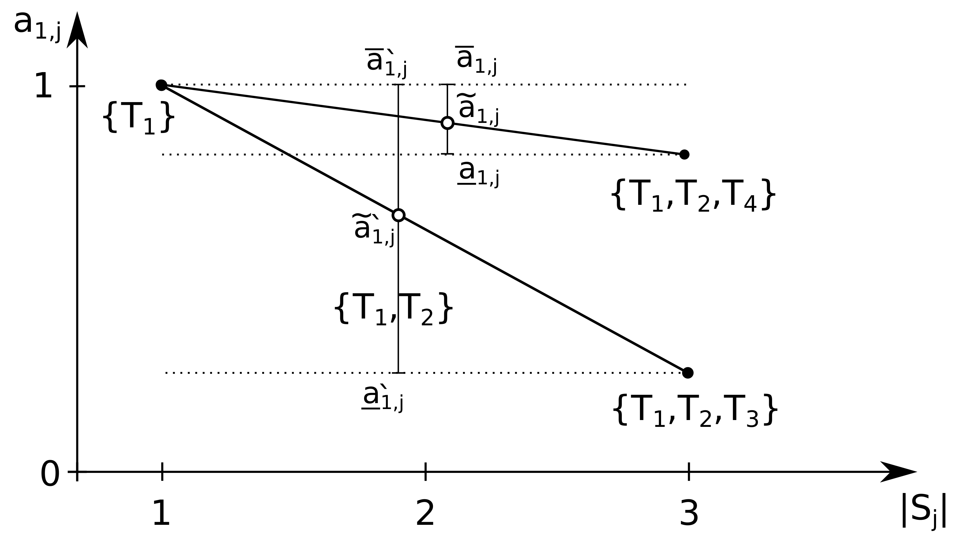
With the assumption that values are measured without any noise and monotonicity constraints, we can claim that $a_{i,j}\in [a_{i,p},a_{i,q}]$ almost surely. We will denote the computed upper and lower boundary values as ${\underline{a}}_{i,j}$ and ${\overline{a}}_{i,j}$, respectively. For the sums of the corresponding values for all tasks in a combination, we will use ${\underline{a}}_j,{\overline{a}}_j,{\tilde{a}}_j$ notation.

Using this method, the value of $a_{i,j}$ can be obtained from multiple different pairs of combinations of $S_p$ and $S_q$. To remove this ambiguity, we will use $S_p$ with the largest number of tasks, such that $S_p\subset S_j$ and $S_q$ with the smallest number of tasks, such that $S_j\subset S_q$. Then, among the possible $S_p$ and $S_q$ with the same size, we will use the one with the minimal boundary interval width ($a_{i,p}-a_{i,q}$). An example when such ambiguity is possible is shown in Figure 3.

5.2. Search Algorithm Acquisition Functions

Implementing a search algorithm requires defining an acquisition function that would select the next task combination for evaluation. The acquisition function matches a single value to every combination based on the confidence interval values of all combinations and the decision on the previous iteration. Then, the search algorithm selects a combination of the highest value of an acquisition function to run in the next iteration.

We have implemented three acquisition functions: probability of improvement, expected improvement and upper confidence bound. The improvement here refers to the increase in task combination speed relative to the value from the previous iteration of the search algorithm. The probability of the improvement function measures the likelihood that the combination has a higher speed than the combination at the current iteration. The expected improvement function accounts not only for the probability but also for the value of the improvement. When the upper confidence bound function is used, the search algorithm would always select the combination with the highest predicted speed value next.

To use these acquisition functions as random functions, we will treat $a_{i,j}$ as random variables. Additionally, we will assume that $a_{i,j}$ are independent and have a normal distribution with the mean value ${\tilde{a}}_{i,j}$ and variance ${\sigma }_{i,j}^2$. As formally we cannot apply these assumptions to the bounded and monotonic values, we will relax the constraints on these values by defining variance as a function of interval bounds in the following way.

Since $a_{i,j}$ is a random variable with a normal distribution, it will exceed ${\tilde{a}}_{i,j}+{\mathsf{\Phi }}^{-1}\left(k\right){\sigma }_{i,j}$ with probability $1-k$, where ${\mathsf{\Phi }}^{-1}\left(k\right)$ is a $k^{th}$-quartile of a standard normal distribution. We will denote the width of $k^{th}$-quartile confidence interval as ${\Delta }_{i,j}$ and compute it as

$${\Delta }_{i,j}=min\{{\overline{a}}_{i,j}-{\tilde{a}}_{i,j},{\tilde{a}}_{i,j}-{\underline{a}}_{i,j}\}$$

(25)

This way, it will ensure that the confidence interval will increase when the distance between the available data points increases and that its shape has a form where the monotonicity constraint holds. As ${\delta }_{i,j}$ can only be positive, we limit k to $0.5<k<1$; then, we can write the variance of $a_{i,j}$ as

$${\sigma }_{i,j}=\frac{{\Delta }_{i,j}}{{\mathsf{\Phi }}^{-1}\left(k\right)}$$

(26)

Later in this paper, we will use k as a tuning parameter for the acquisition function. As the task speed values have a normal distribution, we can claim that combination speed values also have a normal distribution with a mean value of ${\tilde{a}}_j={\sum }_{i\in S_j}{\tilde{a}}_{i,j}$ and variance of ${\sigma }_j^2={\sum }_{i\in S_j}{\sigma }_{i,j}^2$.

We define the probability of improvement ($P{I}_j$), expected improvement ($E{I}_j$) and upper confidence bound ($UC{B}_j$) of a combination $S_j$ in the following way:

$$P{I}_j=\left\{\begin{array}{cc}\mathsf{\Phi }\left(\frac{{\tilde{a}}_j-a^{+}}{{\sigma }_j}\right)\hfill & {\sigma }_j\ne 0\hfill \\ 0\hfill & {\sigma }_j=0,\mathrm{and}{\tilde{a}}_j<a^{+}\hfill \\ 1\hfill & {\sigma }_j=0,\mathrm{and}{\tilde{a}}_j\ge a^{+}\hfill \end{array}\right.$$

(27)

$$E{I}_j=\left\{\begin{array}{cc}({\tilde{a}}_j-a^{+})\mathsf{\Phi }\left(\frac{{\tilde{a}}_j-a^{+}}{{\sigma }_j}\right)+{\sigma }_j\varphi \left(\frac{{\tilde{a}}_j-a^{+}}{{\sigma }_j}\right)\hfill & {\sigma }_j\ne 0\hfill \\ {\tilde{a}}_j-a^{+}\hfill & {\sigma }_j=0\hfill \end{array}\right.$$

(28)

$$UC{B}_j={\tilde{a}}_j+{\sigma }_j$$

(29)

where $\mathsf{\Phi }\left(x\right)$ is a standard normal cumulative distribution function, $\varphi \left(x\right)$ is a standard normal distribution density function and $a^{+}$ denotes the estimated maximum value from the previous iteration. A tuning parameter of these acquisition functions is the probability of the task speed value being outside of the ${\tilde{a}}_{i,j}\pm {\delta }_{i,j}$ interval, i.e., value k. With an increase in parameter k, the value of combination speed variance (${\sigma }_j^2$) decreases.

Simulation results for different acquisition functions are described later in the paper in Section 8.

6. Measuring Task Processing Speed in Experiments

When tasks running in parallel use shared resources, their performances may decrease as bandwidth for these resources is limited and it is being shared between tasks. Examples of such shared resources may include memory bus, shared cache levels, disk bandwidth, network card bandwidth, etc. Such situations can be observed when CPU instruction requiring access to the shared resources may take more CPU cycles to complete, i.e., the rate of finishing instructions (instruction per cycle, IPC) would decrease. IPC is also not specific to any shared resources in particular, but shows the overall speed of processing instructions.

Another reason for performance degradation due to co-scheduling is, when operating the system scheduler, multiple threads are run on the same CPU core sharing cputime. In this case, the IPC of active threads may not change, but their portions of cputime may decrease, resulting in an increase in the overall execution time.

To measure task processing speed (in an absolute value), we propose using metrics such as IPC multiplied by cputime as it is affected by both the operating system scheduler and concurrent access to shared resources. The values of IPC and cputime can be measured during tasks’ runtime with a low overhead by accessing CPU performance counters and thread-specific data provided by operating systems (e.g., ProcFS in Linux).

When processing speed is measured in this way at time t, the unit of work would be CPU instructions ($inst\left(t\right)$) and the unit of time would be CPU cycles $cycl\left(t\right)$. Both of them are provided by CPU performance counters for the time when the task was running in the user space. Cputime $cpu\left(t\right)$ over the sampling period $\Delta t$ would be an unitless value. Assuming that all of these values are cumulative, then we can write the formula for estimating the task processing speed:

$$\nu \left(t\right)=\frac{inst\left(t\right)-inst(t-\Delta t)}{cycl\left(t\right)-cycl(t-\Delta t)}\frac{cpu\left(t\right)-cpu(t-\Delta t)}{\Delta t}$$

(30)

7. Benchmark Applications

To collect experimental data of task processing speed values, we have used the NAS Parallel Benchmark (NPB) [31] and Parsec [32] test suites along with our own test applications. These benchmarks were chosen as they mimic the workload of applications that are common for the HPC field and cover many different types of parallelism patterns’ granularities, inter-thread data exchange, synchronization patterns and have bottlenecks on different types of resources (there are CPU-, memory- and IO-intensive applications).

Due to the assumption of the stationary scheduling problem, among these benchmarks we have selected only those tasks that have constant or periodic speed profiles. The resulting list of benchmark tasks is presented in

Table 1. List of benchmark tasks used in experiments.

Name	Suite	Description
bt	NPB	Block Tri-diagonal solver
ft	NPB	Discrete 3D fast Fourier Transform
lu	NPB	Lower-Upper Gauss-Seidel solver
sp	NPB	Scalar Penta-diagonal solver
fm	Parsec	Frequent Pattern Growth algorithm (freqmine)
so	Parsec	HJM algorithm for pricing swap options (swaption)
vp	Parsec	Image processing pipeline (VIPS library)
sc	Parsec	Online clustering problem in data mining (streamcluster)
ff		Decoding of video file (ffmpeg)
rt		Ray tracing algorithm on CPU

. Datasets of each benchmark were tuned so that each task ran for the same amount of time and on the same computational resources.

For collecting experimental data, we used a single node with an Intel Xeon E5-2630 processor with 10 cores and two threads per core. In the experiments, each task was limited to a certain number of threads by changing parallelism parameters in the benchmark application. Threads were not bound to specific cores and could be migrated between cores by the operating system scheduler (Linux CFS). In all of the experiments, each application had enough memory and swap was never used.

Evaluation of Task Processing Speed Measurements

We used Linux perf (perf_event_open system call) to access CPU performance counters to monitor the number of instructions and number of CPU cycles of each thread in its runtime. Counters values were reported only for the instructions that were running in the user space (as opposed to kernel space). The values of cputime in both the user space and kernel space of each thread were obtained from ProcFS pseudo-filesystem provided by the Linux kernel. These values were used to compute the processing speed of each thread of the running benchmark application. Then, to find the processing speed of the task itself, the values of different threads were averaged.

This approach still allows one to measure the processing speed of each task in the user space and in the kernel space, but with less accuracy. When an instruction takes more CPU cycles due to the shared access to the same resource from another task, the IPC value would be affected. When the application issues an interruption for a system call that is carried out is the kernel space, and it takes more time due to the concurrent access to the shared resources, then this situation would be reflected only by the change in kernel-space cputime. This was carried out deliberately to avoid using two separate processing speed metrics for the kernel space and user space. Additionally, it did not have any noticeable effect on the overall results of experiments.

To show that formula (30) measures the speed of processing, we compared the change of its average value with the change of the total processing time of each benchmark in different conditions. At first, we measured an absolute value of the processing speed and total execution time of each task in ideal conditions, and then again when it was running in combination with other benchmark tasks. After that, we compared the ratio of processing speed in ideal conditions to the processing speed in co-scheduling conditions with the ratio of execution time in co-scheduling conditions to the execution time in ideal conditions. These ratios should be equal for tasks that perform the same total amount of work units (CPU instructions) regardless of the processing speed.

Benchmark tasks that we used perform the same number of CPU instructions regardless of the available resource bandwidth they have, i.e., the amount of work units does not change when benchmarks are running in different combinations (this was shown in our previous paper [33]). This property may not hold when a task performs active waiting on its resources in the user space. In this case, the proposed experiments cannot be used as the number of reported CPU instructions increase when the task was waiting on a resource and not advancing its state. For some benchmarks that use OpenMP for parallelization, we had to ensure that active waiting on thread synchronization primitives was disabled.

We ran these experiments in the following way. For each separate benchmark task that we were measuring, we generated a set of all the possible combinations with other tasks. In these combinations, some tasks may be repeated multiple times, and the number of tasks in each combination could be from 1 to 10. We did not measure all of the combinations, as there are a lot of them and we needed to run each task until completion; instead, we ran 300 of the randomly sampled combinations. For each run, we made sure that the task we were measuring finished the first, otherwise we would measure it in multiple combinations and its speed would not be consistent.

We ran experiments for situations when each task requires the same number of threads and when tasks require a random number of threads. For the same number of threads, we ran two cases, one where each task used two threads and one where they used six threads. In the first case, there were enough CPU cores to run all threads without cputime being shared, and in the second case cputime was shared between threads. When cputime was not shared, its value remained constant and task speed changed only due to the changes in IPC. When cputime was shared, its value may change in different scheduler states and the task speed value would change accordingly. For the situation with the random number of threads, each task may require two to six threads.

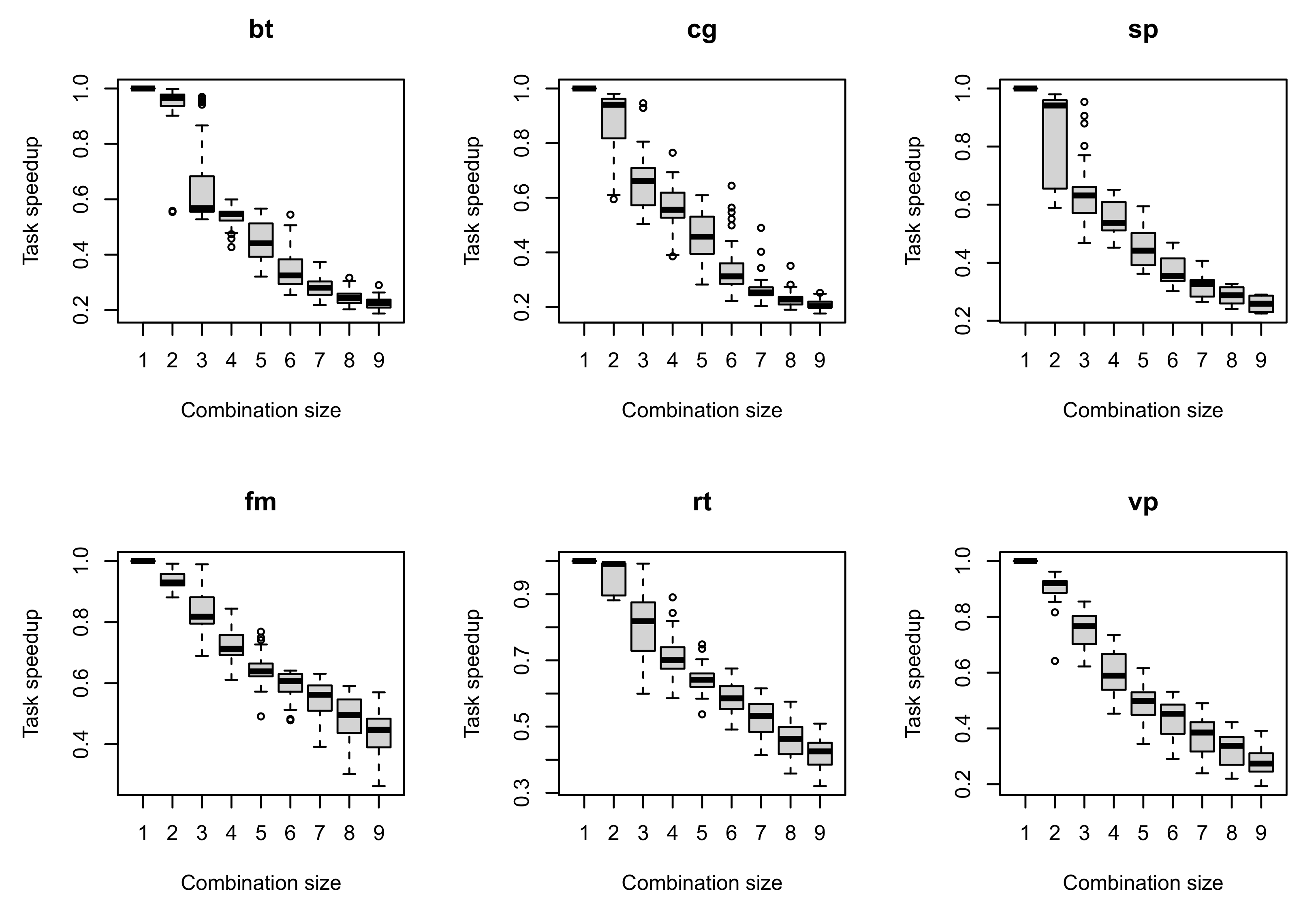
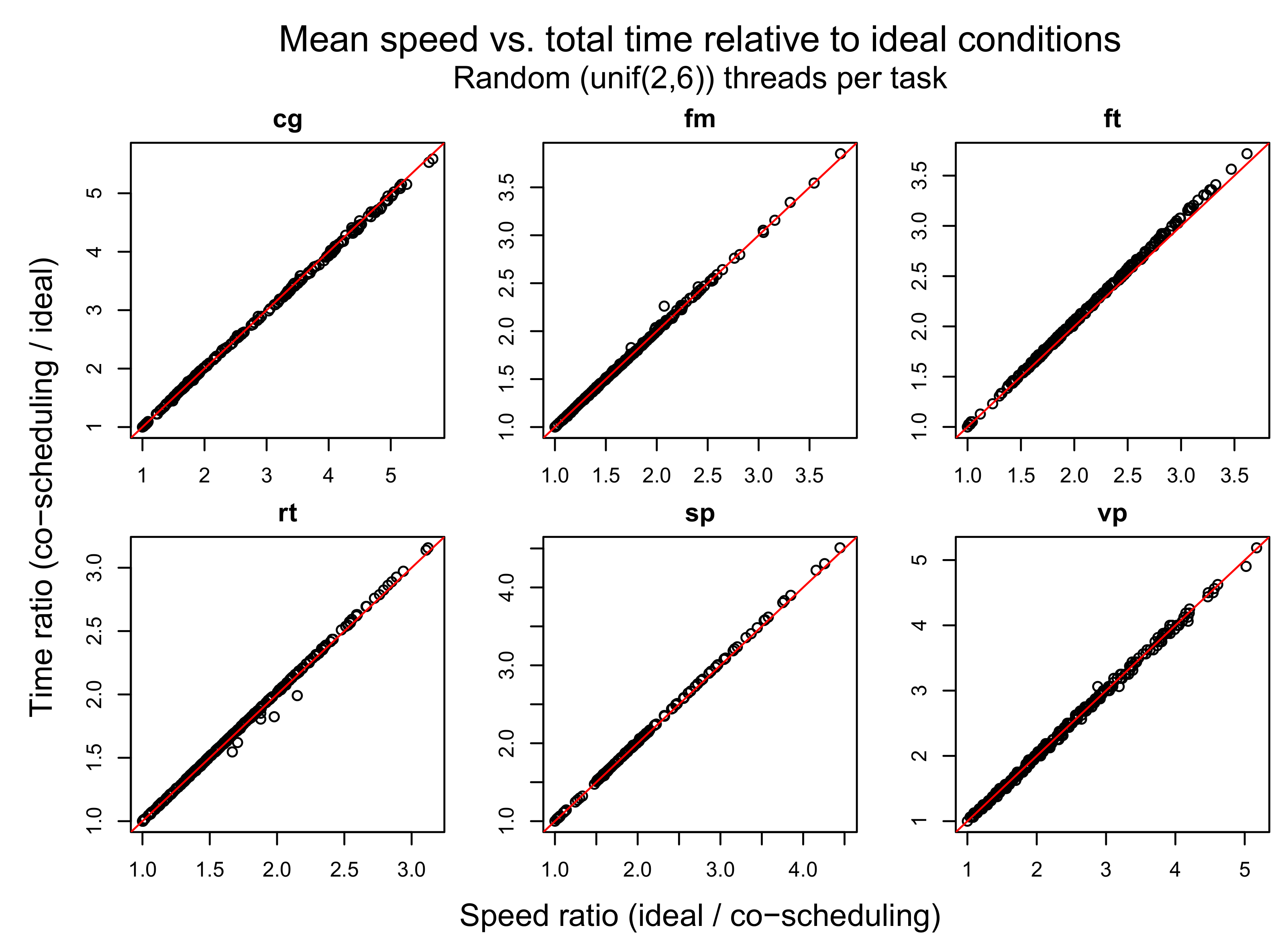
The results of experiments with a random number of threads per task are shown in Figure 4. Since the plots for other experiments’ results look the same, we present them as

Table 2. Linear regression models fitted on experimental data of processing speed ratio as a function of time ratio. The table contains model coefficient and intercept values with R squared values. Data are fitted for the measurement of each benchmark task run in combination with other benchmarks.

Task	2 Threads		6 Threads		From 2 to 6 Threads
	Model	${\mathit{R}}^2$	Model	${\mathit{R}}^2$	Model	${\mathit{R}}^2$
bt	0.984 x + 0.017	0.9997	0.969 x + 0.03	1	0.97 x + 0.029	0.9999
cg	0.984 x + 0.013	0.9996	1.016 x − 0.038	0.9992	1.02 x − 0.042	0.9997
ft	0.995 x + 0.005	0.9996	0.958 x + 0.026	0.9998	0.963 x + 0.032	0.9996
sp	0.994 x + 0.007	0.9998	0.977 x + 0.018	0.9999	0.982 x + 0.017	0.9999
rt	1.015 x − 0.018	0.9943	0.974 x + 0.034	0.9993	0.983 x + 0.02	0.9982
fm	0.993 x + 0.006	0.9999	0.995 x − 0.003	0.9999	0.995 x + 0.005	0.9989
sc	0.958 x + 0.039	0.9986	0.837 x + 0.22	0.9995	0.858 x + 0.188	0.997
vp	1.02 x − 0.008	0.9958	1.016 x + 0.035	0.9501	0.999 x + 0.005	0.9986
ff	0.925 x + 0.065	0.9963	0.843 x + 0.165	0.9956	0.974 x + 0.07	0.9986
so	1.111 x − 0.114	0.9868	0.984 x + 0.025	0.9992	0.984 x + 0.035	0.9964

with linear regression values. The results show that for all benchmarks tasks the ratio of processing times in co-scheduling and ideal conditions matches exactly with task speedup. That is, task speed measured using formula (30) in runtime is proportional to the speed measured after completion (by dividing the work units by the total time).

8. Numerical Simulation Results

To evaluate the search algorithm and FCS strategy and to compare them with an optimal strategy, we implemented simulation software ([34]). It works by generating random task speedup values in each combination ($a_{i,j}$) and task work units ($b_i$). Generated values comply with the constraints defined in Section 3. These values are then used to find the makespan of an optimal strategy by solving the linear programming problem and the makespan of FCS and online search strategies by running their simulations.

The values of $b_i$ were drawn from the uniform distribution from 100 to 200 work units. The values of the task speed in ideal conditions were fixed to 1, so that the task speed in any combination would be the same as the task speedup value. Task speedup values were generated by the following procedure. It works by iterating over all combinations in the order of increasing combination sizes, starting from 2. At each iteration, the maximum allowed speedup of the task is found as a minimum speedup among the combinations of smaller sizes. Then, this value is multiplied by a uniform random number generated between $\alpha$ and 1. The resulting value gives a random speedup value that complies with the monotonicity constraint (1).

The aforementioned $\alpha$ constant corresponds to the maximum slope of the task speed value when the size of the combination increases. We measured task speed as a function of the combination size in experiments, and the results for some benchmarks are shown in Figure 2. Each plot corresponds to a benchmark application running on six cores (out of 20) in combination with other benchmarks running on a random number of cores from 2 to 6. The data were collected in the following way. The combination with the maximum number of tasks was picked at random and the speed of the target task was measured in this combination. Then, a random task was removed from this combination and the target task was measured in a new combination. This process was repeated until the target task was the only task in the combination, i.e., it was running in ideal conditions. At least 30 combinations with the largest size were generated. Each plot shows how the distribution speed value of the task changes depending on the combination size.

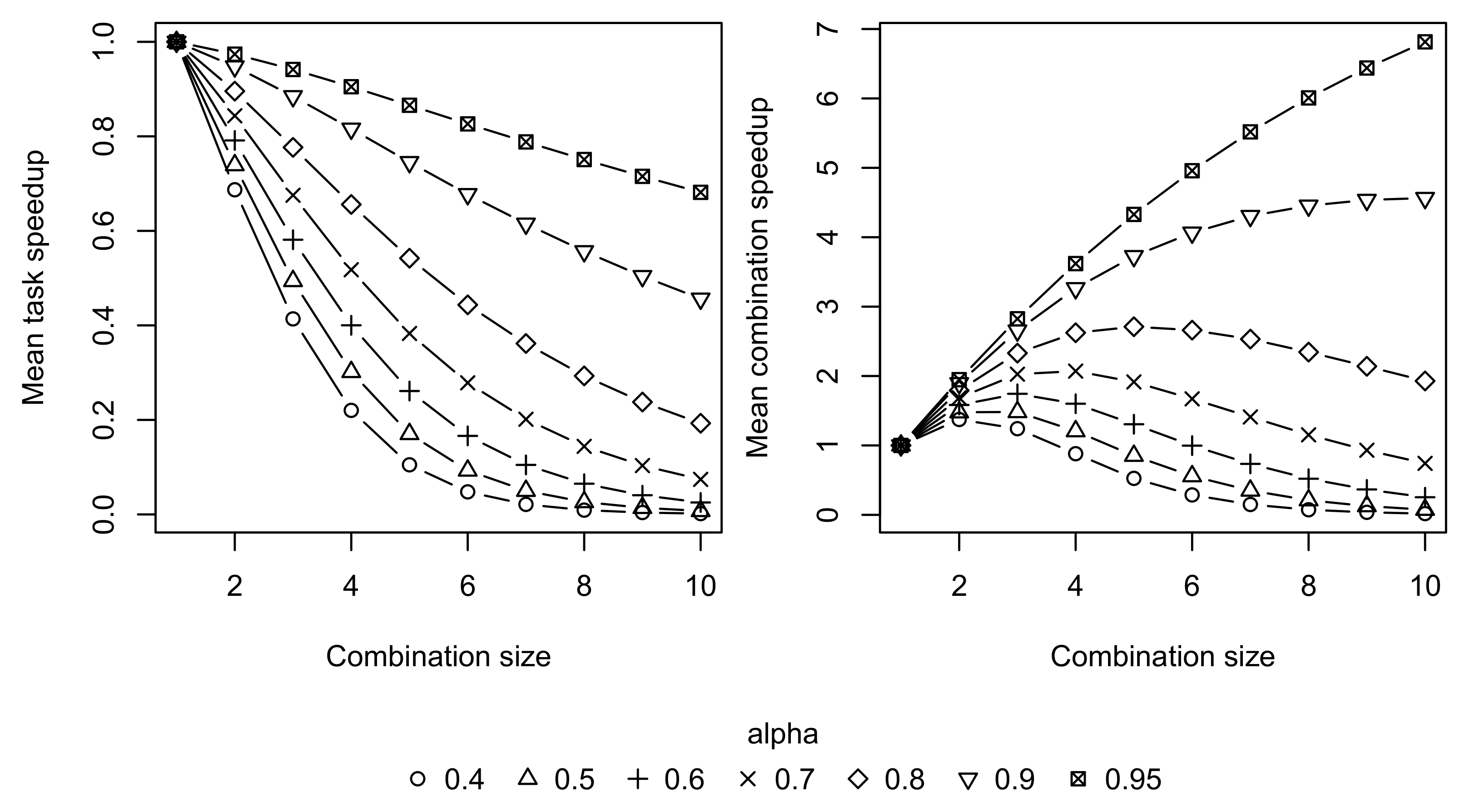
Task speedup and combination speedup values corresponding to different $\alpha$ values are shown in Figure 5. The smaller values of $\alpha$ correspond to the smaller values of task and combination speeds. While all task speed values decrease, their sum, i.e., combination speed, may increase and may reach a peak value for combinations with fewer than n tasks.

In simulations, we used multiple different ranges of $\alpha$ values. Within each range, we chose a value for each task uniformly at random. The range of $\alpha$ from 0.75 to 0.85 was also simulated as it produces the task speed values that are closest to task speedup values measured in the experiments.

We generated 50 problem instances (matrix A and vector b) as described above. Each problem instance had 10 tasks, similar to the experimental setup. We did not vary the maximum number of tasks, as possible curves of combination speed values (right plot in Figure 5) could be generated by changing $\alpha$; increasing the value of n only changes the discretization of these curves.

For these generated problem instances, we simulated FCS and search-based strategies (UCB, PI and EI) and computed their competitive ratios into the optimal strategy. In the search-based strategies, each combination required at least 10 time units of runtime to measure task speed values, which equals to 5–10% of the amount of work in ideal conditions. This value was made deliberately large to exaggerate an effect of sub-optimal decisions of the search algorithm.

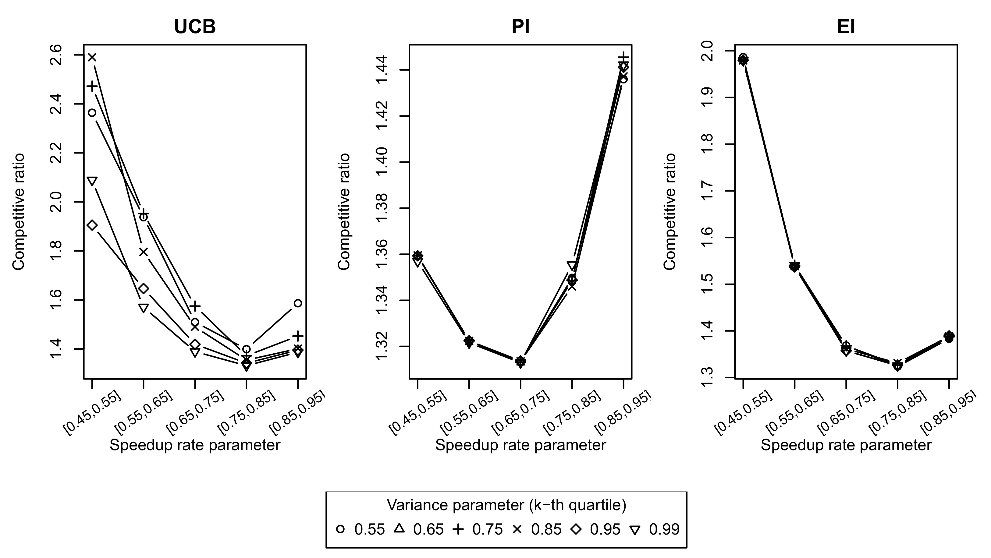
The results of the simulations for these systems are shown in Figure 6 and Figure 7. The competitive ratios of UCB, PI and EI strategies as a function of speedup value ranges ($\alpha$) for different values of variance parameter (k-quartile in (26)) are shown in Figure 6. For the UCB strategy, it can be noticed that its competitive ratio decreases with an increase in k, i.e., with a decrease in confidence interval width. The competitive ratios of PI and EI strategies are not affected by the changes in k. The effect of the $\alpha$ on the competitive ratio is not monotonic for all strategies and the larger deviation from the optimal strategies is reached at the border values of $\alpha$ ranges.

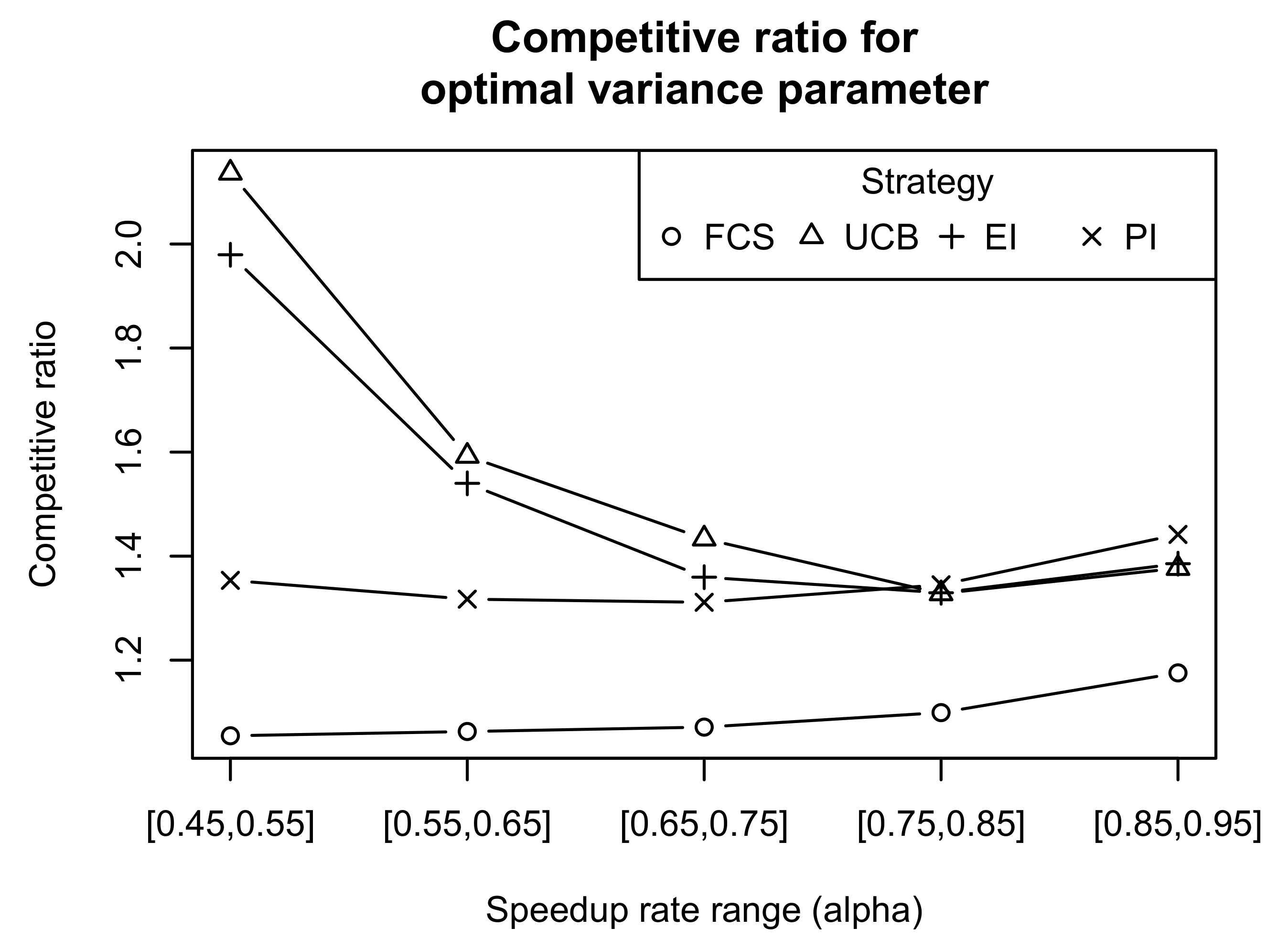
Figure 7 compares the minimal competitive ratio (which is achieved at $k=0.99$) as a function of the $\alpha$ range. As expected, search-based strategies performed worse than the FCS strategy. The maximum competitive ratio of 2.6 was reached by the UCB strategy for $\alpha \in [0.45,0.55]$. For the lower ranges of $\alpha$, the difference between search-based strategies was less pronounced. Based on these simulation results, we can claim that the PI strategy produced better results for all the tested ranges of task speed values. UCB and EI showed worse competitive ratios for larger speedup rate ranges.

9. Discussion

Considering the assumptions of the model, the PI strategy can be used for scheduler implementations, according to simulations. In practice, the model definition must first be improved to account for noisy measurements and the change of task speed values in time. Search-based strategies can be easily adapted to take into account theses assumptions by changing acquisition functions, but showing that the competitive ratio of the FCS strategy obtained in this paper holds for these assumptions is not trivial.

The implementation of search-based scheduling strategies relies on the ability of the operating system scheduler to control task preemption. That is, it should provide an interface for suspending and continuing an execution of running tasks. In Linux, it is possible by using a freezer control group, which is available in kernel releases starting from version 2.6. Stochastic strategies need a preemption interface to iterate over different combinations while measuring the processing speed of each task. To measure these values reliably (within a given confidence interval), some non-interruptible time interval is required, during which tasks would be able to fill CPU caches with their data and perform several computational operations. The problem of minimizing the duration of this time intervals can be considered, but this is outside of the scope of this paper.

The disadvantage of the proposed approach is that there is an exponential number of task combinations ($m=2^n-1$), which results in $O\left(2^n\right)$ computational complexity of all of the strategies, including FCS. However, the number of combinations, in practice, can be reduced due to the following reasons. All tasks that can potentially be run simultaneously must be in a runnable state when the scheduler starts, so that their processing speed can be measured. As the main memory of the node is limited, it limits the number of tasks in combination. Some task combinations can be infeasible, even if they have a small number of tasks. These practical restrictions can be represented in the model by changing a set of combinations from $2^T$ to a custom set of the subset. This would reduce the number of subsets, but would not affect the results obtained in the paper.

The same model of co-scheduling and proposed strategies can be applied to the environments with a single computational node or with multiple computational nodes. In multi-node environment, task combinations may span multiple nodes, but this does not affect the model as constraints imposed on processing speed values do not change. The task processing speed in any combination can be measured in the same way and task preemption implementation would not change as well (given that it is triggered simultaneously on multiple nodes). The model assumption that all tasks must be in a runnable state must also hold for multi-node environments. It can be a limitation for practical implementations as well as it would mean that mapping of all tasks threads or processes to nodes must be computed in advance, before any task scheduling strategies would start. The alternative that does not have this assumption and would allow one to implement co-scheduling is to introduce live migrations of the task processes between nodes. This approach may have practical limitations and strategies proposed in the paper cannot be trivially transformed to account for it.

Other scheduling strategies that potentially may lead to practical results can also be considered within this model definition and assumptions. For example, values of the total amount of work for each task (vector b) may be considered as known quantities. In practice, this can be achieved by analysing historical data of previous runs of the same task. With the assumptions that each task processes constant amount of work units, these values can be reliably used for making scheduling decisions.

It is possible to implement the proposed strategies as an extension to a batch scheduler (e.g., as a SLURM extension) or as a stand-alone scheduler, which would work on top of the existing batch scheduler. The latter approach may require a user-writable control group to implement task preemption. Alternatively, task preemption can be implemented using signals, which does not require interventions from privileged system users. Linux performance (perf) counters can be used for measuring the task processing speed, which in general does not require any privileged access. There are no restrictions on the applications that can be run using this scheduling approach, as it does not require any code or binary file modifications. The implementation of the scheduler is outside of the scope of this paper and will be addressed in future work.

10. Conclusions

In this paper, we defined a model for solving the co-scheduling problem and proposed multiple scheduling strategies: an optimal strategy, an online strategy (FCS) and heuristic strategies (EI, PI and UCB). The optimal solution was found by reducing the problem to a linear programming problem, which requires all task processing speeds and amounts of work to be known in advance. The FCS strategy is defined with the assumption that only the task processing speed is available, while required work units are unknown. Heuristic strategies work with the assumption that no information is available at start, but the task processing speed can be measured over the task runtime.

We showed theoretically that the FCS strategy produces schedules that are at most two times worse than the optimal strategy. This allowed us to solve the co-scheduling problem using heuristic strategies that approximate FCS. We defined these strategies as implementations of stochastic optimization algorithms with different acquisition functions. To apply these optimization algorithms, we defined a non-deterministic version of the co-scheduling problem by treating each task processing speed value as a random variable and relaxing constraints on its value by defining its variance.

We used numerical simulations to compare all strategies with an optimal strategy and to show how heuristic strategies behave for tuning parameters with different values and problem inputs. The results showed that the PI strategy produced lower values of completive ratios than the EI and UCB strategies for almost all problem input data.

We also proposed a method for measuring a task’s processing speed over its runtime and evaluated it using benchmark HPC applications in different environments. We showed that this method measures values with high accuracy, which allows one to apply the proposed scheduling strategies in scheduler implementations.

There are multiple possible directions for improving this work in both theoretical and practical aspects that we plan to address in future work. For example, an additional constraint of task precedence can be considered, which would make the model applicable to solving workflow scheduling problems. The stochastic definition of the problem can also be improved by accounting for noisy measurements of the task processing speed and for their change in time. We are also working on the scheduler implementation that would manage task co-scheduling running on top of an existing batch scheduler.