Article

Association Analysis of Deep Genomic Features Extracted by Denoising Autoencoders in Breast Cancer

1
Department of Biochemistry and Medical Genetics, College of Medicine, Faculty of Health Sciences, University of Manitoba, Winnipeg, MB R3E 0J9, Canada
2
Research Institute in Oncology and Hematology, CancerCare Manitoba, Winnipeg, MB R3E 0V9, Canada
3
Department of Computer Science, University of Manitoba, Winnipeg, MB R3T 2N2, Canada
*
Author to whom correspondence should be addressed.
Cancers 2019, 11(4), 494; https://doi.org/10.3390/cancers11040494
Submission received: 17 March 2019 / Revised: 3 April 2019 / Accepted: 4 April 2019 / Published: 7 April 2019
(This article belongs to the Special Issue Application of Bioinformatics in Cancers)

Abstract

:
Artificial intelligence-based unsupervised deep learning (DL) is widely used to mine multimodal big data. However, there are few applications of this technology to cancer genomics. We aim to develop DL models to extract deep features from the breast cancer gene expression data and copy number alteration (CNA) data separately and jointly. We hypothesize that the deep features are associated with patients’ clinical characteristics and outcomes. Two unsupervised denoising autoencoders (DAs) were developed to extract deep features from TCGA (The Cancer Genome Atlas) breast cancer gene expression and CNA data separately and jointly. A heat map was used to view and cluster patients into subgroups based on these DL features. Fisher’s exact test and Pearson’ Chi-square test were applied to test the associations of patients’ groups and clinical information. Survival differences between the groups were evaluated by Kaplan–Meier (KM) curves. Associations between each of the features and patient’s overall survival were assessed using Cox’s proportional hazards (COX-PH) model and a risk score for each feature set from the different omics data sets was generated from the survival regression coefficients. The risk scores for each feature set were binarized into high- and low-risk patient groups to evaluate survival differences using KM curves. Furthermore, the risk scores were traced back to their gene level DAs weights so that the three gene lists for each of the genomic data points were generated to perform gene set enrichment analysis. Patients were clustered into two groups based on concatenated features from the gene expression and CNA data and these two groups showed different overall survival rates (p-value = 0.049) and different ER (Estrogen receptor) statuses (p-value = 0.002, OR (odds ratio) = 0.626). All the risk scores from the gene expression and CNA data and their concatenated one were significantly associated with breast cancer survival. The patients with the high-risk group were significantly associated with patients’ worse outcomes (p-values ≤ 0.0023). The concatenated risk score was enriched by the AMP-activated protein kinase (AMPK) signaling pathway, the regulation of DNA-templated transcription, the regulation of nucleic acid-templated transcription, the regulation of apoptotic process, the positive regulation of gene expression, the positive regulation of cell proliferation, heart morphogenesis, the regulation of cellular macromolecule biosynthetic process, with FDR (false discovery rate) less than 0.05. We confirmed DAs can effectively extract meaningful genomic features from genomic data and concatenating multiple data sources can improve the significance of the features associated with breast cancer patients’ clinical characteristics and outcomes.

1. Introduction

Advanced hardware technologies have highly increased computational power, which makes the implementation of computation-consuming algorithms possible. At the same time, the development of biological technologies has greatly reduced the cost of genomic sequencing, which produced a huge amount of high-dimensional genomic data. Under these circumstances, bioinformatics becomes an exciting research field for researchers to explore the possibility to interpret genomic data using advanced computational technologies [1].
Different types of high-dimensional genomic data have been associated with cancer clinical characteristics and outcomes. The most commonly used ones are gene expression data and copy number alteration (CNA) data [2]. The activity of gene expression in tumor tissues is quite different from that in normal tissues [3] and has been established to have the ability to distinguish the characteristics of cancers [4]. There are some repeated segments in normal DNA, and during the process of cancer development, the repeated number of the segments may be changed due to abnormal DNA replication in tumor cells. This phenomenon is called copy number alteration [5]. CNA may result in chromosome structure changes in the forms of duplication or deletion in DNA segments. It has been shown that CNA plays an important role in the development of many types of cancers including breast cancer [6]. Therefore, it is highly necessary to mine the prognostic and diagnostic significance of the genome-wide cancer genomic data. From a clinical point of view, the prognosis of the genomic factors is always a necessary consideration because of its importance in making treatment plans [7]. In previous studies, prognosis significance was evaluated mainly based on clinical features, such as tumor grades and tumor subtypes [7] and molecular features, such as expression related gene signatures (e.g., PAM50 subtypes) [8,9]. Results from these studies showed that the gene signatures tend to have better prognosis significance than traditional pathological assessment [7]. This might be due to the integration ability of these gene signatures. For instance, PAM50 can combine the information from the tumor stage, tumor grade and tumor subtype together [9]. However, the known gene signatures are only based on single genomic data source such as gene expression. This might be not adequate since other types of genomic data such as copy number alterations should also include important cancer prognosis information [9]. Advanced algorithms now give us new tools to explore the possibility of integrating different data sources together. For example, Chi, et al. identified several genes and pathways with a high prognostic significance for young breast cancer patients based on their gene expression and copy number alteration data using a graph-based machine learning (ML) method [9].
Traditional ML methods such as artificial neural networks (ANN) and support vector machines (SVM) may suffer some problems in dealing with the high-dimensional, noisy and massive genomic data [10]. Recently, a special case of ANN with more nodes and layers has emerged as an efficient method to handle these high-dimensional and noisy data. The idea of ANN was originated from the information processing and communication patterns in a human nervous system [11]. As the new development of the traditional ANN, deep learning (DL) presents a large group of interconnected artificial neurons with many more layers. Like other learning methods, DL could be implemented in a supervised or unsupervised way, which depends on whether the input data is labeled or not. Although both supervised and unsupervised DL algorithms have been successfully applied to the analysis of genomic data, they could be used to solve different biology problems. Supervised learning algorithms are often used to predict gene functions and gene-gene interactions or to identify new driver genes [12], while unsupervised learning algorithms are often used to cluster the strong signals in the data [13,14]. Among the unsupervised learning algorithms, autoencoder is a new technology that uses the data itself as the learning objective or label. Therefore, it is also known as self-labeled or self-supervised deep learning. Traditional autoencoders may face the invalid learning problem when the number of hidden nodes is larger than the input size. To avoid this potential risk, denoising autoencoders (DAs) came up with the solution of adding some noise into the input data on purpose.
Vincent, et al. brought the concept of DAs into DL and built a specialized feature extraction DL architecture [15]. The key idea of DAs as mentioned above is to add random noise into the raw data before it is input into the network. After the encode and decode processes, the raw data would be reconstructed from the noisy data, while the compact and efficient representations from the raw data could be learned as well [15]. These representations are the DAs-based genomic features.
DL as a special case of ML and ANN has been applied to mine deep information from complex genomic data and has generated interesting results [16]. Its high integration and reconstruction abilities give us large flexibility to combine different types of genomic data to extract valuable information from them. It has been expected that deep features extracted by DL models would perform better in clinical association and prognosis prediction than standard gene or pathway signatures [17]. For example, Tan, et al. reported a deep feature representing ER status and a deep feature with high prognosis significance based on breast cancer gene expression data [13]. These deep features were constructed by a DAs and performed better in the downstream analyses [13]. However, these studies were based on only a single genomic source.
This study aims to extract the integrated features from both the gene expression and CNA data by a concatenated DAs model. As a comparison, we also built a standard DAs model to extract deep features from gene expression and CNA data separately. The comparisons were made in terms of the performance in association analysis as well as prognosis analysis. The study design and analysis procedures are shown in Figure 1.

2. Materials and Methods
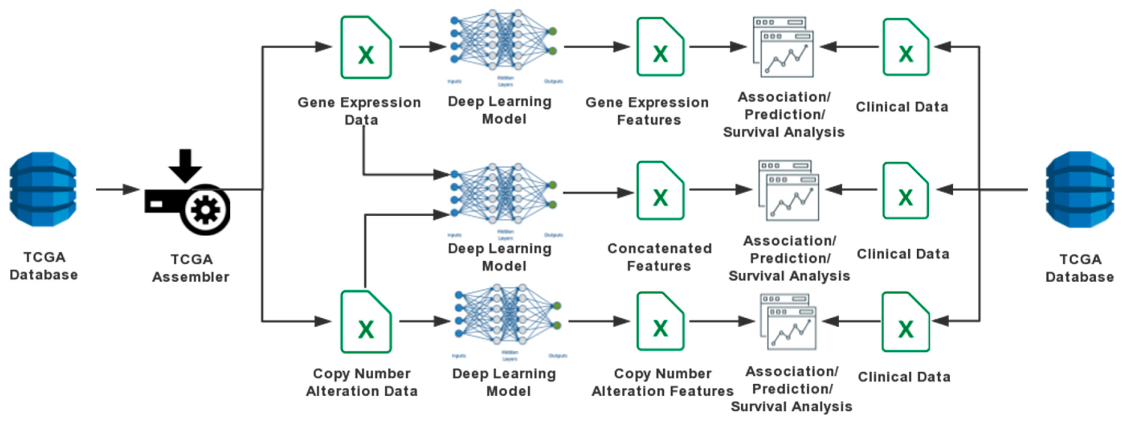
2.1. Data Sources

Datasets used in this study came from The Cancer Genome Atlas (TCGA) [18], which is one of the most comprehensive genomic databases. TCGA provides 1098 breast cancer patients’ clinical data along with their genomic data. These genomic data include gene expressions, CNA, protein expressions, micro RNA (miRNA) expressions, and somatic mutations.
For gene expression data, the sequencing, alignment, quality control and quantification were performed previously [18]. Using the TCGA-Assembler tool [19], we downloaded the gene expression raw count, then filtered out unexpressed genes and those genes with a count per million (CPM) less than 1 in 3 patients. We performed normalization of the data using Upper Quartile Fragments per Kilobase of transcript per Million mapped reads (FPKM-UQ) [20]. FPKM-UQ is a modified FPKM algorithm in which the total read count is replaced by the 75th percentile read count for a given sample.
Similar to the gene expression data, upstream processes of CNA data were done previously as well [18]. Using the downloaded chromosome-region specific log2 copy number data, we calculated the gene-level CNA values using the TCGA-Assembler tool. Several data cleaning procedures such as removing all-NAs were also performed to avoid potential format issues in the follow-up analysis.
After normalization and preprocessing, there were 18,163 genes from each of the 1095 patients left for gene expression data and 23,563 genes from the 1098 patients left for CNA data. To keep the gene dimension and scale matched in the two data sources, both of them were linearly transformed into a range between 0 and 1, resulting in the decreasing of the data dimension to 16,197 (genes) × 1085 (patients) for both data sources.

2.2. DA Models

Two DAs models were developed using Keras [21] with Tensorflow [22] as the backend to extract deep genomic features. One model was for feature extraction from a single genomic source, named as one-input DAs model (Figure 2). The other, named as the two-input DAs model (Figure 3), was for concatenated feature extraction from the integrated genomic sources.

2.2.1. One-Input DAs Model

This architecture was composed of one input layer, one fully connected encode hidden layer with 100 nodes which were chosen to be the deep features used in this study and one decode layer which uses the transpose of encoding layer’ weights. This procedure can be formulated as below:
encode = sigmoid (W × input + b)
decode = sigmoid (W’ × encode + b’)
where W is the weight metrics between the layers with the size of 16,197 × 100, b is the bias for each node, and the sigmoid function is sigmoid (x) = 1 / (1 + e−x). The counterparts with the superscript refer to the transpose metrics. A dropout layer was added after the encode layer, which randomly set 50% of the output of encode layer to 0 to prevent overfitting. The encode item was chosen to be the activity values of the deep features in this model.

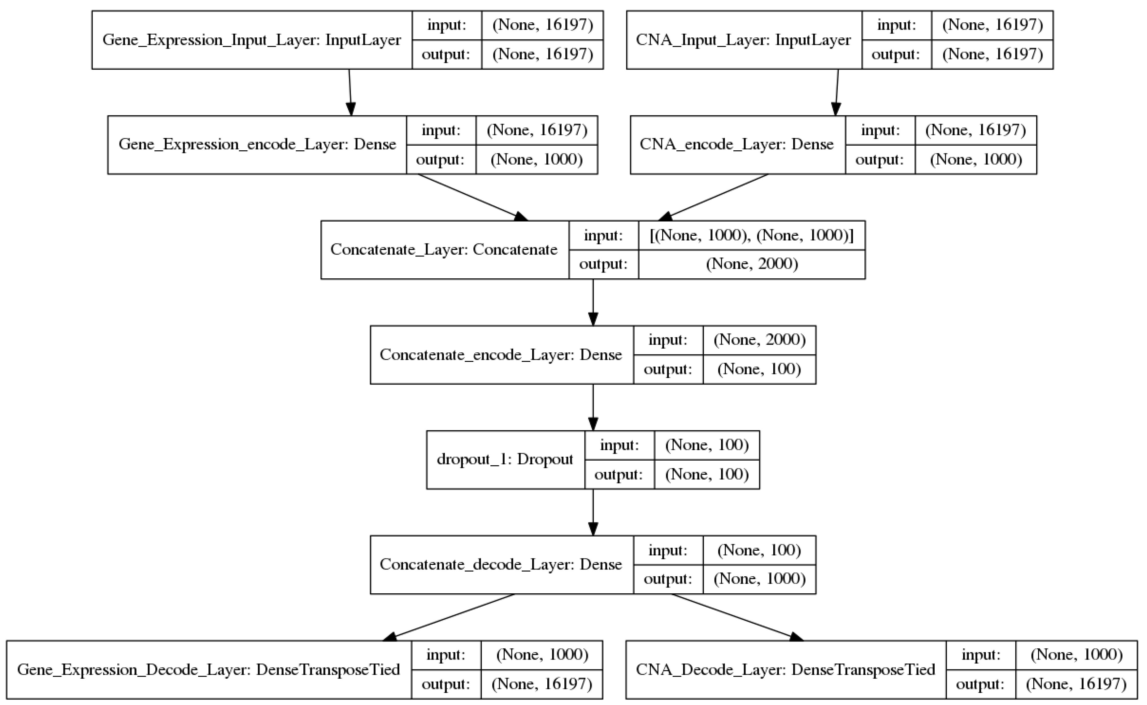
2.2.2. Two-Input DAs Model

Literally, the two-input DAs model contained two input layers, followed by one encode layer with 1000 nodes for each input layer, then followed by a concatenated layer, and another encode layer with 100 nodes which were chosen to be the deep concatenated features. Finally, there were two decode layers. The procedure can be formulated as follow:
input1_encode1 = sigmoid (input1_W1 × input1 + input1_b1)
input2_encode1 = sigmoid (input2_W1 × input2 + input2_b1)
concate_encode1 = concatenate (input1_encode1, input2_encode1)
concate_encode2 = sigmoid (concate_W2 × concate_encode1+ concate_b2)
output1 = sigmoid (input1_W1 × concate_encode2 + input1_b1)
output2 = sigmoid (input2_W1 × concate_encode2 + input2_b1)
where input1_W1, input2_W1, and concate_W2 are the weight metrics between the layers with the size of 16,197 × 1000, 16,197 × 1000, 2000 × 100 respectively. The input1_b1, input2_b1, and concate_b2 are the biases for each node. The counterparts with superscript refer to the transpose metrics. A dropout layer was added after concate_encode2 layer, which randomly set 50% of the output of that layer to 0. The concate_encode2 was chosen to be the activity values of the deep features in this model.

2.3. Train the Models

Before the training process, the input data sets were disrupted by a noise factor of 0.25, which is the proportion of the number of genes in the data sources. These genes were selected randomly and their values were set to 0. The binary cross-entropy function shown below was used to measure the difference between the input layer and the output layer:
L (input, output) = −(1/N) Σ (inputk × log(outputk) + (1 − inputk) × log(1 − outputk))
where L (input, output) is the binary cross-entropy, K is the index of batches, N is the total number of batches. Thus, the training task is to minimize the L (input, output).
For the optimizer, e.g., the strategy to update the weights and bias so that the minima could be found, we selected stochastic gradient descent (SGD), which has several arguments to be set freely. After having different trials, the learning rate was finally set to 0.1; the batch size and epoch were set to 64 and 100 respectively. The models were finally trained under the parameters mentioned above. The activity values and weight metrics related to deep features were read out.

2.4. Visualization and Clustering

Heatmap3 [23] was used to visualize the activity values of these deep feature sets. We used the complete linkage function in the hierarchical clustering process and visual-guided criteria by analysis of the dendrogram to decide the number of clusters. First, the clinical data downloaded from TCGA were carefully scanned and the most clinical-relevant characteristics such as pathological status (T, N, M), tumor stage, estrogen receptor (ER) status, progesterone receptor (PR) status, human epidermal growth factor receptor 2 (HER2) status, triple negative status, and PAM50 subtypes (i.e., Luminal A, Luminal B, Basal-like, HER2-enriched, and Normal-like) were extracted. These clinical characteristics were shown as the sidebar of the heat map.

2.5. Association Analysis

To test whether the identified patient clusters are associated with known clinical and molecular characteristics, we applied both Fisher’s exact test and Pearson’ Chi-square test.
Survival differences between the identified patients groups were evaluated by Kaplan–Meier (KM) curves. Furthermore, associations between each deep feature in the three feature sets (gene expression, CNA, the concatenated one) and patient’s overall survival was assessed using Cox’s proportional hazards (COX-PH) model [24]. The hazard function is
h(t) = h0 (t) × exp (bx)
where t represents the survival time. b is the coefficient which measures the impact of the covariate x. Later, a risk score for each feature set was generated from the COX-PH coefficients:
r = Σ (bi × ai)
where r is the risk score, bi is the coefficient from the COX-PH model and ai is the related activity value of the given feature. Afterward, the risk scores were binarized into high-risk and low-risk groups using R package xtile function with a prob parameter set to 0.55, which means we use the 55% quantile as the cutoff to bin the patients into the high-risk and low-risk groups. Finally, the survival differences between these two groups were evaluated by the KM curve.

2.6. Gene Sets Enrichment Analysis

For each of the three DAs models for gene expression, CNA and their concatenated one, we traced back their gene-level weights based on
Wg = W × B
where W is the 16,197 × 100 dimensional weights that were extracted from a given DAs model previously. B is the vector of COX-PH coefficients. The gene-specific weights Wg were filtered by a cutoff 0.01, which resulted in the three selected gene lists with 6954, 5381 and 6297 genes, respectively. Finally, the three gene lists were used to perform gene set enrichment analysis (GSEA) by the Enricr tool [25] to identify the up-regulated and down-regulated pathways. Kyoto Encyclopedia of Genes and Genomes (KEGG) [26] and Gene Ontology (GO) [27] Biological Process 2018 version were chosen to be the reference gene sets.

3. Results

Based on the normalized and processed breast cancer genomic data, our models were trained and the activity values of the 100 deep features for each of the three data sets as well as the weights matrices were extracted (Table 1). Then we clustered these activity values for each of the three data sets. Overall, there were no clear patterns shown in the deep features from a single genomic source (gene expression or CNA data). However, patients were roughly clustered into 2 groups according to the activity values of the concatenated deep features (Figure 4).
Results from the association tests between the two patient groups and their clinical characteristics are shown in Table 2. The two patient groups showed significant survival (Figure 5) and ER status difference (Table 2) with p-values 0.049 and 0.002, respectively, which mean that the concatenated features have learned the ER information and performed well in predicting patient’s prognosis. The odds ratio of ER status is 0.626, indicating that the second group tends to be associated with ER-negative patients. From the KM plot (Figure 5), we can see that the patients in Group 2 suffered from a poor prognosis, which happens to be associated with ER-negative status. It has been shown that ER-negative breast cancer patients usually have a poor prognosis.
According to the results of COX-PH models, the high-risk scores generated from each of the three deep feature sets are all significantly associated with a poor overall survival with p-values less than 1 × 10⁻⁵ (Table 3). The concatenated features showed a higher hazard ratio (HR) with 95% confidence interval (CI) (1.27, 1.16–1.40) than gene expression features (1.009, 1.005–1.013) and CNA features (1.23, 1.15–1.32). These results indicated that the risk scores from the deep features, especially the concatenated risk score, predict patient’s poor prognosis. The similar patterns were observed in KM plots (Figure 6), where the patient group with high-risk scores always suffered from a poor prognosis.
GSEA using the 6,297 genes selected based on the concatenated deep feature set showed that the AMP-activated protein kinase (AMPK) signaling pathway in the KEGG family was significantly down-regulated with a false discovery rate (FDR) less than 0.05, and several GO-based regulation processes, such as the regulation of DNA-templated transcription, the regulation of nucleic acid-templated transcription, the regulation of apoptotic process, the positive regulation of gene expression, the positive regulation of cell proliferation, and the regulation of cellular macromolecule biosynthetic process were significantly enriched as well, with an FDR less than 0.05 (Table 4).
AMPK is an important cellular metabolism and energy homeostasis regulator in mammalian tissues. It is situated in the center of a signaling network which contains tumor suppressors such as LKB1, TSC2 and p53 [25]. Some evidence has been reported that AMPK plays an anti-tumorigenic role and a lot of work are ongoing to involve agonists of AMPK for cancer treatment [28]. Furthermore, all those enriched GO regulation processes are critical as hallmarks in cancer occurrence and progression [29].

4. Discussion

In building the DA model, one of the key parameters we need to set up is the noise level used to partially destroy the inputs. We tried to add different levels of noise (e.g., 0%, 10%, 25% and 50%) into the DA model. Similar to the observations made by Vincent et al. [15], we also found that the more noise was added the better the network learns dependencies between the features. With low noise levels, the learned features do not stand out. As we set the noise level at 0.25, denoising training can capture more distinctive deep features.
Comparing with conventional breast cancer biomarkers, such as CA15-3 for measuring how breast cancer treatment is working and looking for cancer that has come back or recurred, after treatment [30], and NCC-ST-439 for measuring breast cancer progression [31], the explanation of the deep genomic features or biomarkers from the DA model for breast cancers is more complicated. Each of the extracted deep features is a high-level summary of the raw features or conventional biomarkers. These high-level features or biomarkers can be more robust against noise in the conventional biomarkers. Furthermore, these high-level features can potentially significantly improve the breast cancer outcome prediction by integrating information from both breast cancer histology images and genomic biomarkers [32]. The extracted features based on the proposed deep learning model can be also used to predict the statuses of malignancy, relapse, and reactivity for anticancer if the related data sources are available. We will explore the method in other large data sets and cancer types in the future. This can further validate the usefulness of the method for risk stratification of cancer patients.
In order to extract robust deep features using the proposed DA model, we took a strategy to add noise into the input genomic data by the partial corruption of the input pattern. It is expected that the learned deep features from the partially destroyed inputs can yield almost the same representation of the raw genomic data. In order to further boost the performance of using the learned deep features to predict breast cancer outcome or traits, another interesting strategy is to incorporate the prior knowledge about breast cancer hallmarks, which can be represented by a few molecular or signaling networks [33], into the deep learning procedure. This can be potentially implemented in different ways. For example, the interaction information among different genes or mutations collected in the molecular or signaling network databases can be used to assign the weights in different layers of the network among different neurons. We will explore the interesting strategy in future studies.

5. Conclusions

In this study, we showed that unsupervised DAs as an effective model to extract meaningful deep genomic features from either single- or multi- genomic sources from breast cancer patients. These features were significantly associated with the breast cancer ER status and had the prognosis significance. We also showed that the concatenated deep features were enriched by breast cancer relevant pathways.
This study can be improved in two potential ways. The first one is to develop new DAs model structures such as stacking more layers into DAs or adding a regression layer to make it supervised [34]. The second one is to combine all types of possible data sources together, such as somatic mutation data, protein expressions, miRNA expressions, etc. We will explore these ideas in future analyses.

Author Contributions

Q.L. and P.H. were involved in the conceptualization, development of methodologies and manuscript writing; P.H. was involved in supervision, project administration and funding acquisition.

Funding

This research was supported in part by Canadian Breast Cancer Foundation, Natural Sciences and Engineering Research Council of Canada, Manitoba Health Research Council and University of Manitoba.

Conflicts of Interest

The authors declare no conflict of interest.

Abbreviations

DLDeep learning
CNACopy number alteration
DAsDenoising autoencoders
TCGAThe Cancer Genome Atlas
KMKaplan-Meier
COX-PHCox’s proportion hazard
OROdds ratio
AMPKAMP-activated protein kinase
FDRFalse discovery rate
GSEAGene sets enrichment analysis
MLMachine learning
ANNArtificial neural network
SVMSupport vector machine
EREstrogen receptor
miRNAMicro RNA
CPMCount per million
FPKM-UQUpper quartile fragments per kilobase of transcript per Million mapped reads
SGDStochastic gradient descent
KEGGKyoto Encyclopedia of Genes and Genomes
GOGene Ontology

References

  1. Lesk, A.M. Introduction to Bioinformatics, 3rd ed.; Oxford University Press: Oxford, UK, 2008. [Google Scholar]
  2. Bergamaschi, A.; Kim, Y.H.; Wang, P.; Sørlie, T.; Hernandez-Boussard, T.; Lonning, P.E.; Tibshirani, R.; Borresen-Dale, A.L.; Pollack, J.R. Distinct patterns of DNA copy number alteration are associated with different clinicopathological features and gene-expression subtypes of breast cancer. Genes Chromosomes Cancer 2006, 45, 1033–1040. [Google Scholar] [CrossRef]
  3. Ramaswamy, S.; Tamayo, P.; Rifkin, R.; Mukherjee, S.; Yeang, C.H.; Angelo, M.; Ladd, C.; Reich, M.; Latulippe, E.; Mesirov, J.P.; et al. Multiclass cancer diagnosis using tumor gene expression signatures. Proc. Natl. Acad. Sci. USA 2001, 98, 15149–15154. [Google Scholar] [CrossRef] [Green Version]
  4. Sorlie, T.; Tibshirani, R.; Parker, J.; Hastie, T.; Marron, J.S.; Nobel, A.; Deng, S.; Johnsen, H.; Pesich, R.; Geisler, S.; et al. Repeated observation of breast tumor subtypes in independent gene expression data sets. Proc. Natl. Acad. Sci. USA 2003, 100, 8418–8423. [Google Scholar] [CrossRef] [PubMed] [Green Version]
  5. Wu, H.T.; Hajirasouliha, I.; Raphael, B.J. Detecting independent and recurrent copy number aberrations using interval graphs. Bioinformatics 2014, 30, i195–i203. [Google Scholar] [CrossRef] [Green Version]
  6. Beroukhim, R.; Mermel, C.H.; Porter, D.; Wei, G.; Raychaudhuri, S.; Donovan, J.; Barretina, J.; Boehm, J.S.; Dobson, J.; Urashima, M.; et al. The landscape of somatic copy-number alteration across human cancers. Nature 2010, 463, 899–905. [Google Scholar] [CrossRef] [Green Version]
  7. Boughorbel, S.; Al-Ali, R.; Elkum, N. Model Comparison for Breast Cancer Prognosis Based on Clinical Data. PLoS ONE 2016, 11, e0146413. [Google Scholar] [CrossRef] [PubMed]
  8. Nielsen, T.O.; Parker, J.S.; Leung, S.; Voduc, D.; Ebbert, M.; Vickery, T.; Davies, S.R.; Snider, J.; Stijleman, I.J.; Reed, J.; et al. A comparison of PAM50 intrinsic subtyping with immunohistochemistry and clinical prognostic factors in tamoxifen-treated estrogen receptor-positive breast cancer. Clin. Cancer Res. 2010, 16, 5222–5232. [Google Scholar] [CrossRef] [PubMed]
  9. Chi, C.; Murphy, L.C.; Hu, P. Recurrent copy number alterations in young women with breast cancer. Oncotarget 2018, 9, 11541–11558. [Google Scholar] [CrossRef] [PubMed] [Green Version]
  10. Auria, L.; Moro, R.A. Support Vector Machines (SVM) as a Technique for Solvency Analysis; DIW Discussion Papers 811; DIW Berlin, German Institute for Economic Research: Berlin, Germany, 2008. [Google Scholar]
  11. Olshen, A.B.; Venkatraman, E.S.; Lucito, R.; Wigler, M. Circular binary segmentation for the analysis of array-based DNA copy number data. Biostatistics 2004, 5, 557–572. [Google Scholar] [CrossRef]
  12. Schadt, E.E.; Lamb, J.; Yang, X.; Zhu, J.; Edwards, S.; Guhathakurta, D.; Sieberts, S.K.; Monks, S.; Reitman, M.; Zhang, C.; et al. An integrative genomics approach to infer causal associations between gene expression and disease. Nat. Genet. 2005, 37, 710–717. [Google Scholar] [CrossRef] [Green Version]
  13. Tan, J.; Ung, M.; Cheng, C.; Greene, C.S. Unsupervised feature construction and knowledge extraction from genome-wide assays of breast cancer with denoising autoencoders. Pac. Symp. Biocomput. 2014, 20, 132–143. [Google Scholar]
  14. Guyon, I.; Elisseeff, A. Feature Extraction, Foundations and Applications: An introduction to feature extraction. Stud. Fuzziness Soft Comput. 2006, 207, 1–25. [Google Scholar]
  15. Vincent, P.; Larochelle, H.; Bengio, Y.; Manzagol, P.A. Extracting and composing robust features with denoising autoencoders. In Proceedings of the 25th International Conference on Machine Learning, Helsinki, Finland, 5–9 July 2008; ACM: New York, NY, USA, 2008; pp. 1096–1103. [Google Scholar]
  16. Khan, J.; Wei, J.S.; Ringnér, M.; Saal, L.H.; Ladanyi, M.; Westermann, F.; Berthold, F.; Schwab, M.; Antonescu, C.R.; Peterson, C.; et al. Classification and diagnostic prediction of cancers using gene expression profiling and artificial neural networks. Nat. Med. 2001, 7, 673–679. [Google Scholar] [CrossRef] [PubMed]
  17. Angermueller, C.; Pärnamaa, T.; Parts, L.; Oliver, S. Deep Learning for Computational Biology. Mol. Syst. Biol. 2016, 12, 878. [Google Scholar] [CrossRef] [PubMed]
  18. Tomczak, K.; Czerwińska, P.; Wiznerowicz, M. The Cancer Genome Atlas (TCGA): An immeasurable source of knowledge. Wspolczesna Onkol. 2015, 19, A68–A77. [Google Scholar] [CrossRef] [PubMed]
  19. Zhu, Y.; Qiu, P.; Ji, Y. TCGA-assembler: Open-source software for retrieving and processing TCGA data. Nat. Methods 2014, 11, 599–600. [Google Scholar] [CrossRef]
  20. Bullard, J.H.; Purdom, E.; Hansen, K.D.; Dudoit, S. Evaluation of statistical methods for normalization and differential expression in mRNA-Seq experiments. BMC Bioinform. 2010, 11, 94. [Google Scholar] [CrossRef] [PubMed]
  21. Chollet, F. Building Autoencoders in Keras. The Keras Blog. 2016. Available online: https://blog.keras.io/building-autoencoders-in-keras.html (accessed on 20 January 2019).
  22. Abadi, M.; Barham, P.; Chen, J.; Chen, Z.; Davis, A.; Dean, J.; Devin, M.; Ghemawat, S.; Irving, G.; Isard, M.; et al. TensorFlow: A System for Large-Scale Machine Learning. In Proceedings of the 12th USENIX Symposium on Operating Systems Design and Implementation (OSDI’16), Savannah, GA, USA, 2–4 November 2016; pp. 265–284. [Google Scholar]
  23. Wu, G.; Xing, M.; Mambo, E.; Huang, X.; Liu, J.; Guo, Z.; Chatterjee, A.; Goldenberg, D.; Gollin, S.M.; Sukumar, S.; et al. Somatic mutation and gain of copy number of PIK3CA in human breast cancer. Breast Cancer Res. 2005, 7, R609–R616. [Google Scholar] [CrossRef] [Green Version]
  24. Ching, T.; Zhu, X.; Garmire, L.X. Cox—Nnet: An artificial neural network method for prognosis prediction on high—Throughput omics data. PLoS Comput. Biol. 2016, 14, e1006076. [Google Scholar] [CrossRef]
  25. Chen, E.Y.; Tan, C.M.; Kou, Y.; Duan, Q.; Wang, Z.; Meirelles, G.V.; Clark, N.R.; Ma’ayan, A. Enrichr: Interactive and collaborative HTML5 gene list enrichment analysis tool. BMC Bioinform. 2013, 14, 128. [Google Scholar] [CrossRef]
  26. Ogata, H.; Goto, S.; Sato, K.; Fujibuchi, W.; Bono, H.; Kanehisa, M. KEGG: Kyoto encyclopedia of genes and genomes. Nucleic Acids Res. 1999, 27, 29–34. [Google Scholar] [CrossRef]
  27. Ashburner, M.; Ball, C.A.; Blake, J.A.; Botstein, D.; Butler, H.; Cherry, J.M.; Davis, A.P.; Dolinski, K.; Dwight, S.S.; Eppig, J.T.; et al. Gene ontology: Tool for the unification of biology. Nat. Genet. 2000, 25, 25–29. [Google Scholar] [CrossRef]
  28. Giordanetto, F.; Karis, D. Direct AMP-activated protein kinase activators: A review of evidence from the patent literature. Expert Opin. Ther. Pat. 2012, 22, 1467–1477. [Google Scholar] [CrossRef]
  29. Hanahan, D.; Weinberg, R.A. Hallmarks of cancer: The next generation. Cell 2011, 144, 646–674. [Google Scholar] [CrossRef]
  30. Harris, L.; Fritsche, H.; Mennel, R.; Norton, L.; Ravdin, P.; Taube, S.; Somerfield, M.R.; Hayes, D.F.; Bast, R.C., Jr. American Society of Clinical Oncology 2007 update of recommendations for the use of tumor markers in breast cancer. J. Clin. Oncol. 2007, 25, 5287–5312. [Google Scholar] [CrossRef]
  31. Miyahara, E.; Toi, M.; Wada, T.; Yamada, H.; Osaki, A.; Yanagawa, E.; Toge, T. The expression of NCC-ST-439, a tumor marker, in human breast cancer patients. Gan No Rinsho 1990, 36, 2023–2026. [Google Scholar]
  32. Mobadersany, P.; Yousefi, S.; Amgad, M.; Gutman, D.A.; Barnholtz-Sloan, J.S.; Vega, J.E.V.; Brat, D.J.; Cooper, L.A.D. Predicting cancer outcomes from histology and genomics using convolutional networks. Proc. Natl. Acad. Sci. USA 2018, 115, E2970–E2979. [Google Scholar] [CrossRef] [Green Version]
  33. Wang, E.; Zaman, N.; Mcgee, S.; Milanese, J.S.; Masoudi-Nejad, A.; O’Connor-McCourt, M. Predictive genomics: A cancer hallmark network framework for predicting tumor clinical phenotypes using genome sequencing data. Semin. Cancer Biol. 2015, 30, 4–12. [Google Scholar] [CrossRef] [Green Version]
  34. Vincent, P.; Larochelle, H.; Lajoie, I.; Bengio, Y.; Manzagol, P.A. Stacked denoising autoencoders: Learning useful representations in a deep network with a local denoising criterion. J. Mach. Learn. Res. 2010, 11, 3371–3408. [Google Scholar]
Figure 1. A flowchart illustrating the analysis procedures in this study.
Cancers 11 00494 g001
Figure 2. The one-input denoising autoencoders model. There are two hidden layers in the encode phase and two decode layers. The input can be either gene expression data or copy number alteration data.
Cancers 11 00494 g002
Figure 3. The two-input DAs model. There are two hidden layers in the encode phase and one decode layer. Concatenation was performed between the two encode layers.
Cancers 11 00494 g003
Figure 4. The clustering of activity values of concatenated deep features extracted under the noise factor of 0.25. The columns are the 1085 patients and the rows are the 100 deep features. The sidebar contains the corresponding clinical information of the patients. Values are clustered by both columns and rows.
Cancers 11 00494 g004
Figure 5. The Kaplan–Meier (KM) plot of the two patient groups clustered by the concatenated features.
Cancers 11 00494 g005
Figure 6. The KM-plots for risk scores based on the deep feature sets. (A) Gene expression data; (B) copy number alteration data; (C) the concatenated data.
Cancers 11 00494 g006
Table 1. The size and organization of deep features obtained from the models. The size and structure of the deep features extracted from gene expression data and copy number alteration data by the two denoising autoencoders (DAs) models.
ModelData SourceDeep Features (Noise Factors = 0.25)
One-input DAsGene expressionsActivity values1085 × 100
weights16,197 × 100
Copy number alterationsActivity values1085 × 100
weights16,197 × 100
Two-input DAsGene expressions
Copy number alterations
Activity values1085 × 100
weights16,197 × 100
Table 2. The results of clinical association analysis. * patients were classified as young (age < 40) and old (age ≥ 40) groups.
Clinical CharacteristicsFisher’s Exact p-ValueChi-Square Test p-Value
Pathological T0.690.69
Pathological N0.950.96
Pathological M0.950.94
Tumor Stage0.930.93
ER Status0.0020.002
PR Status1.000.99
HER Status0.430.44
Age *0.580.67
Triple Negative Status0.150.17
Tumor Subtype0.350.36
Table 3. Cox’s proportional hazards (COX-PH) results for risk scores.
Risk ScoreHRLower.95_HRUpper.95_HRp-Value
Gene expression1.0091.0051.0131.06 × 10−5
CNA1.231.151.327.86 × 10−9
Concatenated1.271.161.405.62 × 10−7
Table 4. The gene set enrichment analysis using Enricr.
Gene Setsp-ValueAdjusted p-Value
regulation of transcription, DNA-templated2.25 × 10−70.001
regulation of nucleic acid-templated transcription6.03 × 10−50.04
regulation of apoptotic process6.19 × 10−50.04
positive regulation of gene expression5.89 × 10−50.04
positive regulation of cell proliferation4.78 × 10−50.04
AMPK signaling pathway_Homo sapiens_hsa041526.08 × 10−50.018

