Active Control of a Small-Scale Wind Turbine Blade Containing Magnetorheological Fluid


Abstract
:1. Introduction
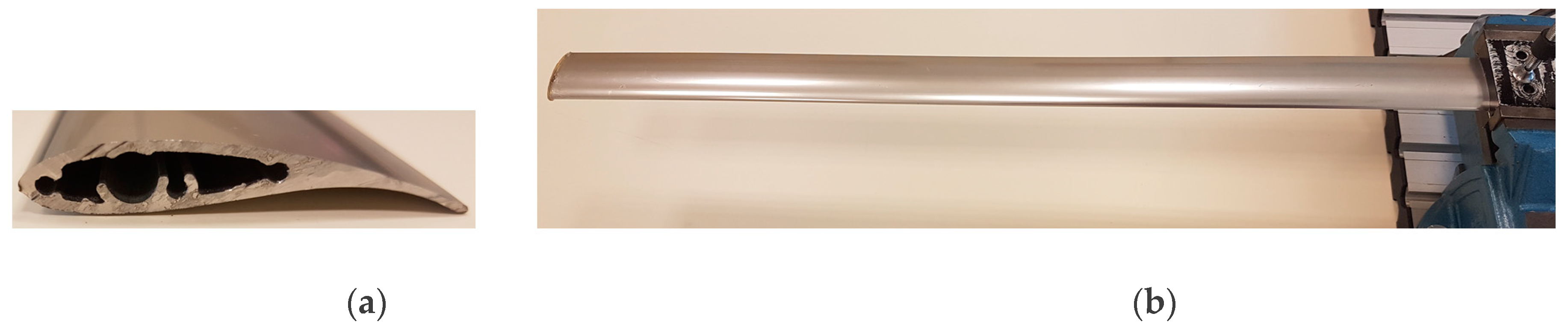
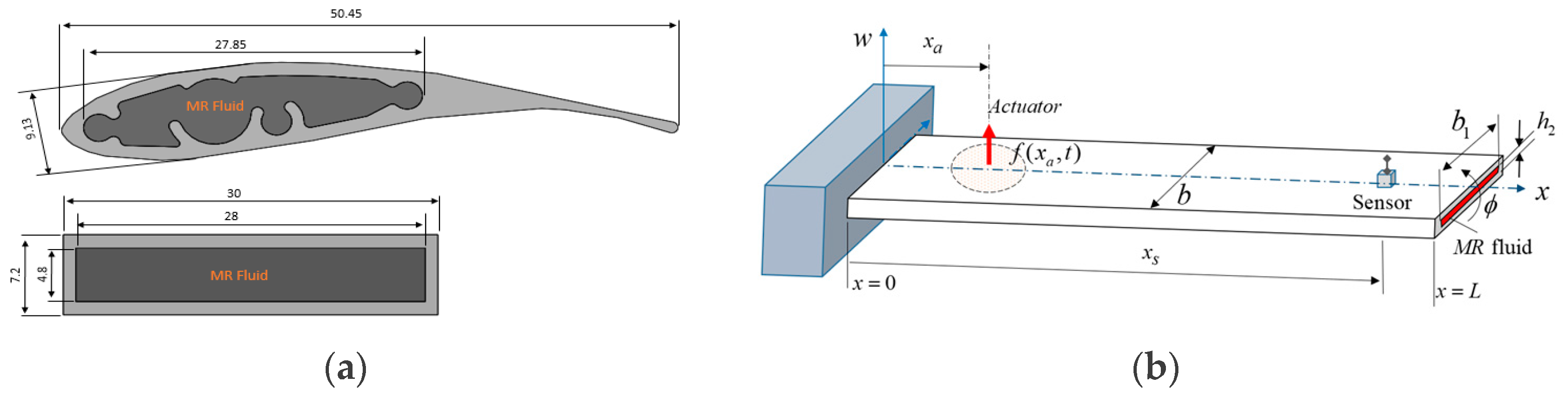
2. Elastic Blade Structure
2.1. Equivalent Beam Model
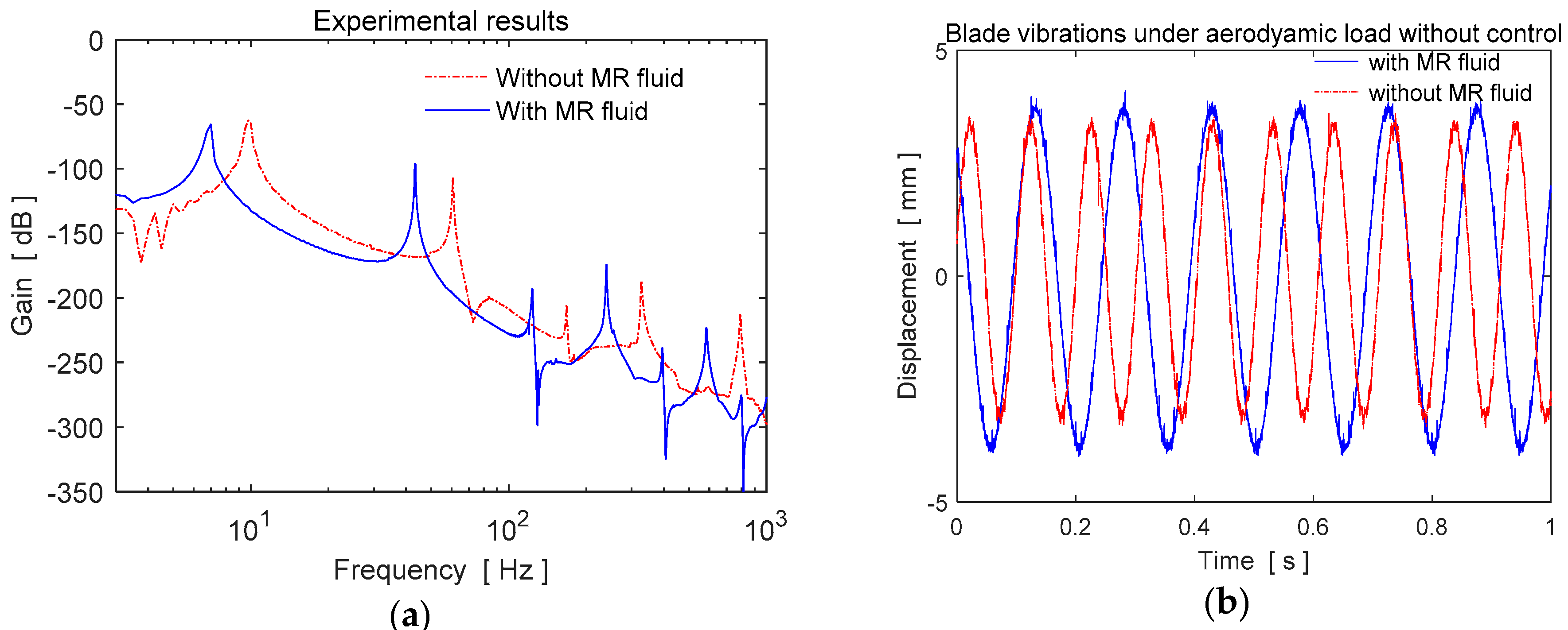
2.2. Natural Frequency Analysis
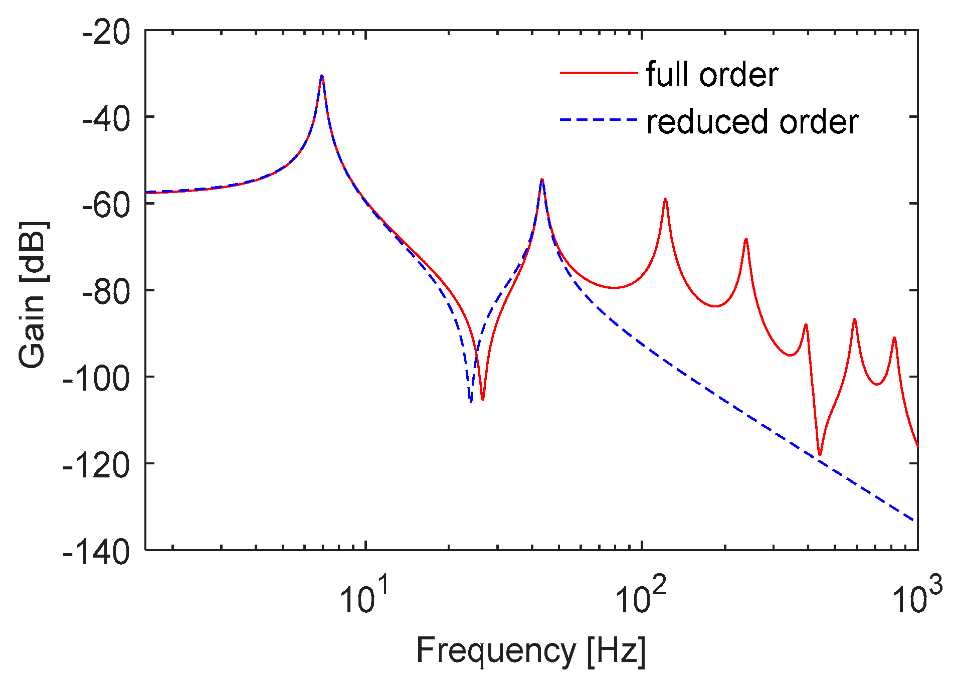
2.3. State Space Model
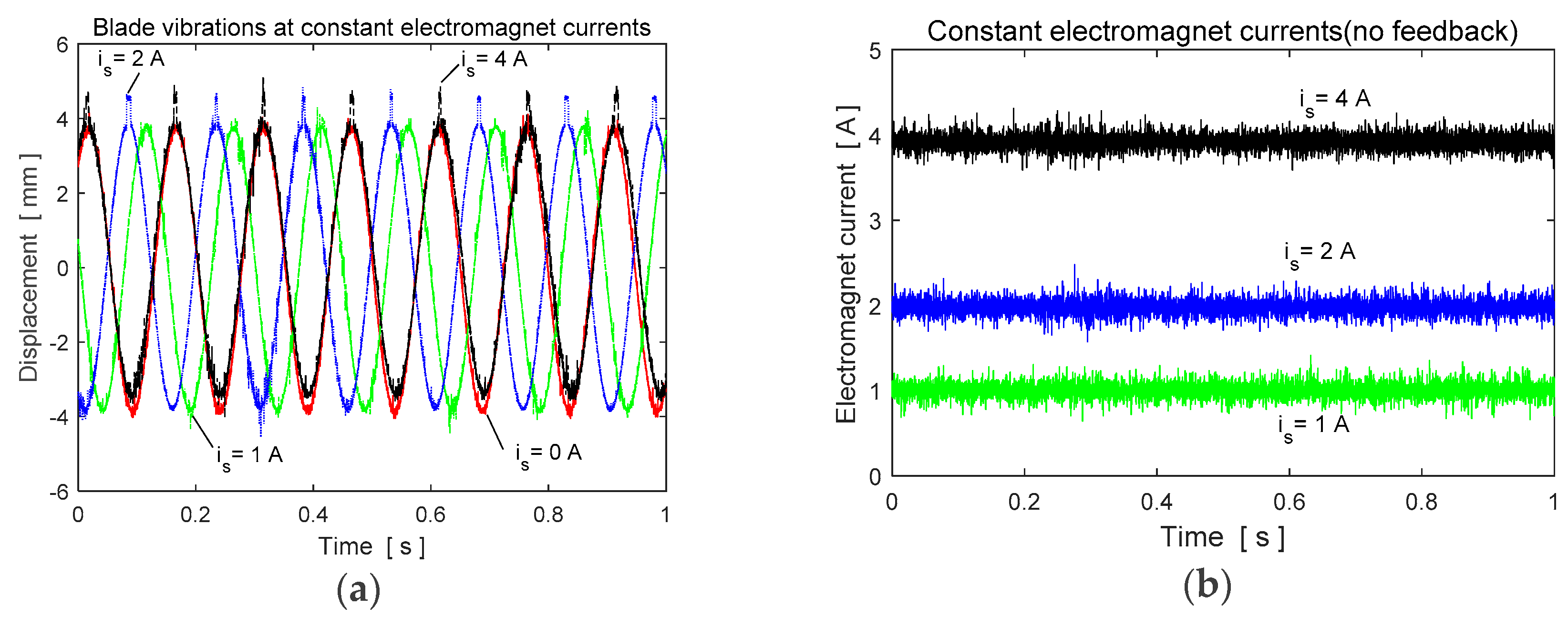
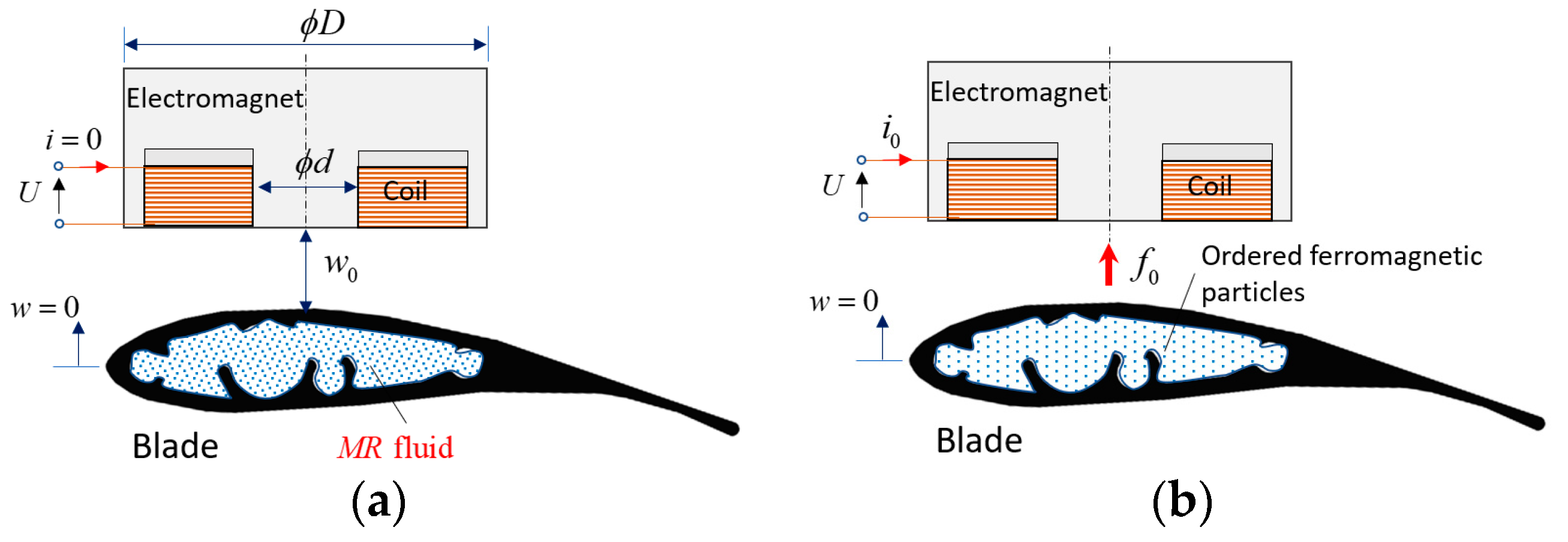
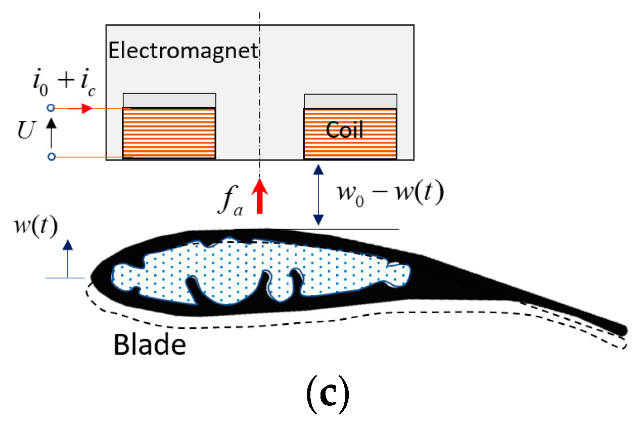
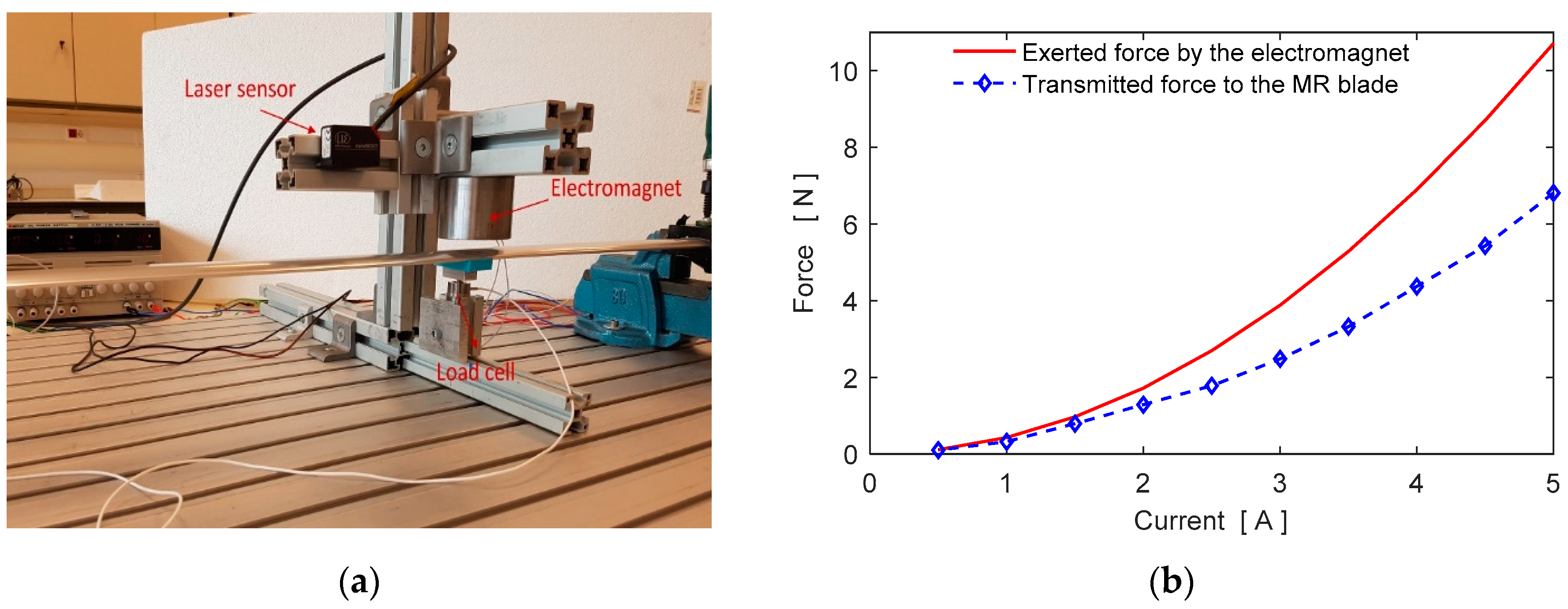
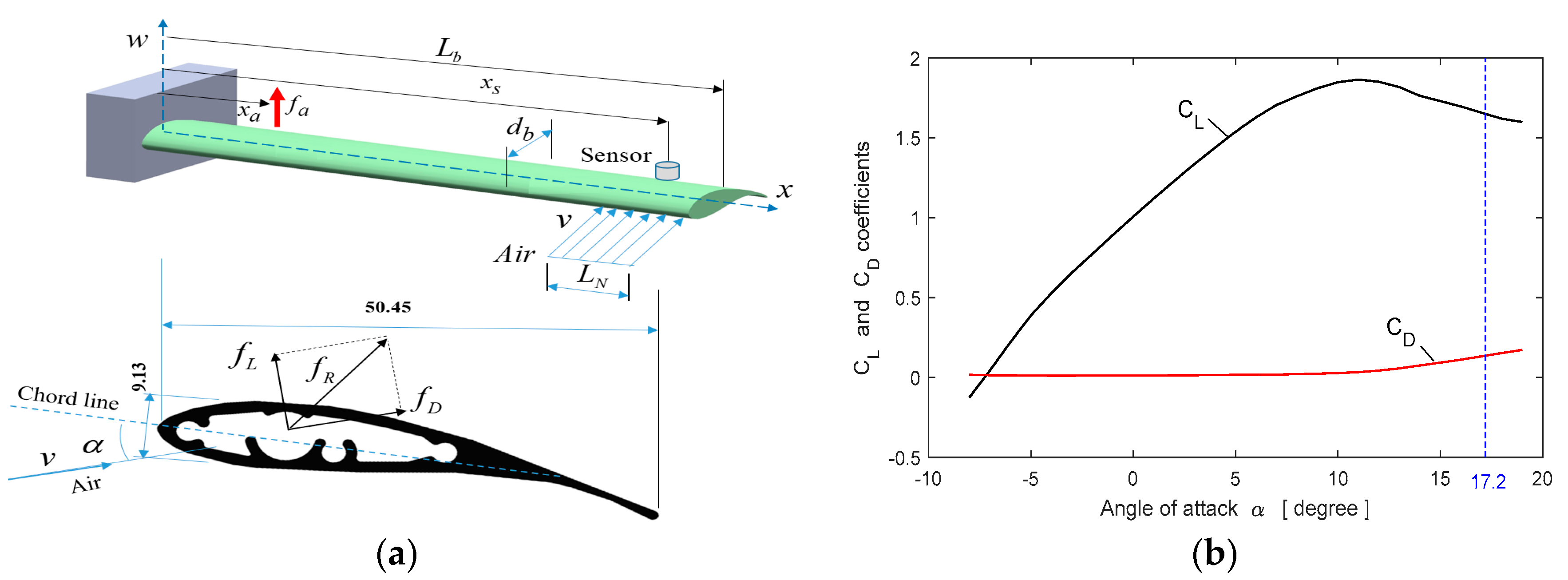
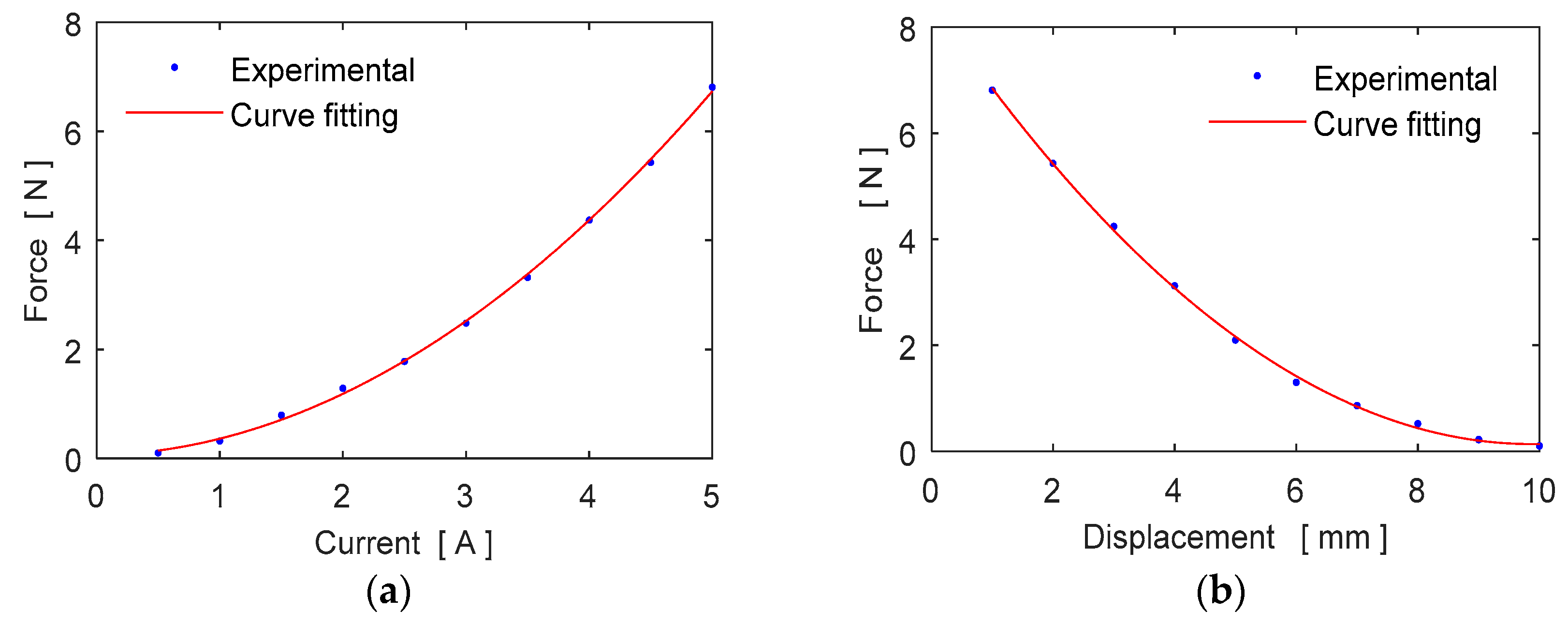
2.4. Force Characterization
2.5. Aerodynamic Load
3. Control Principle
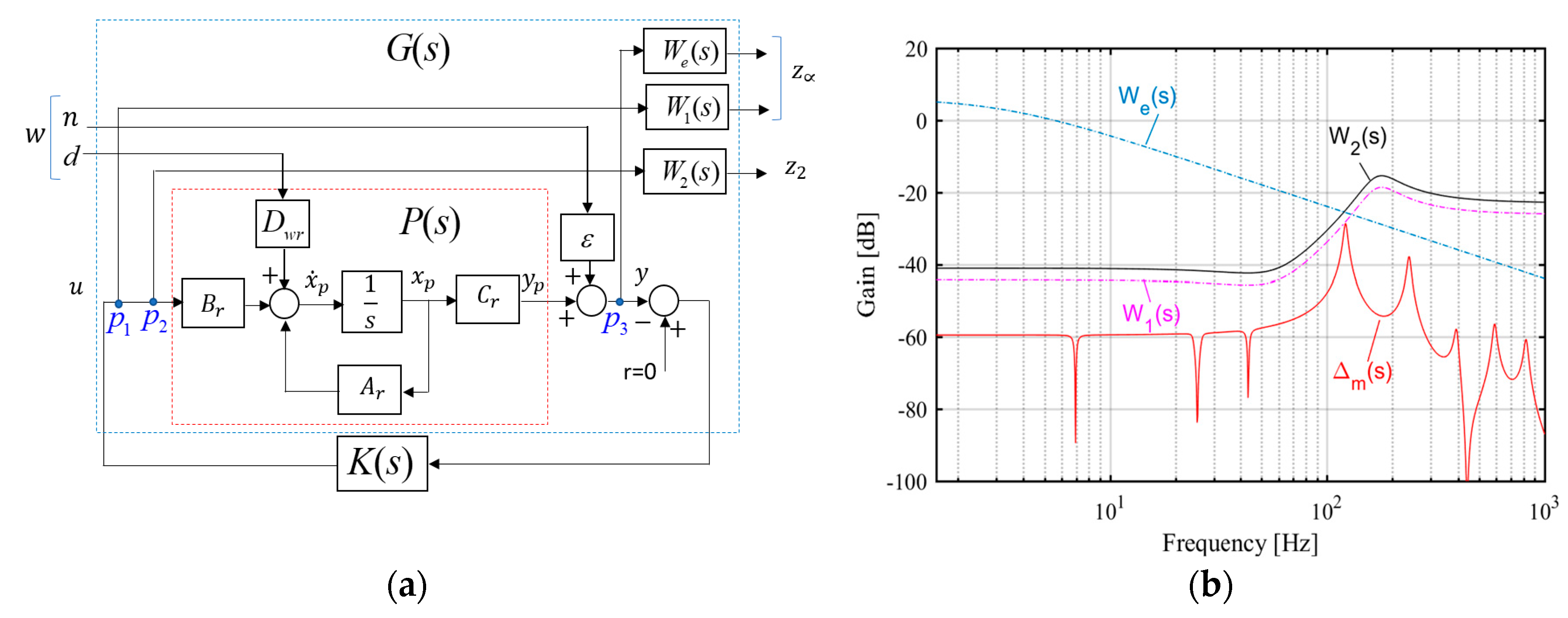
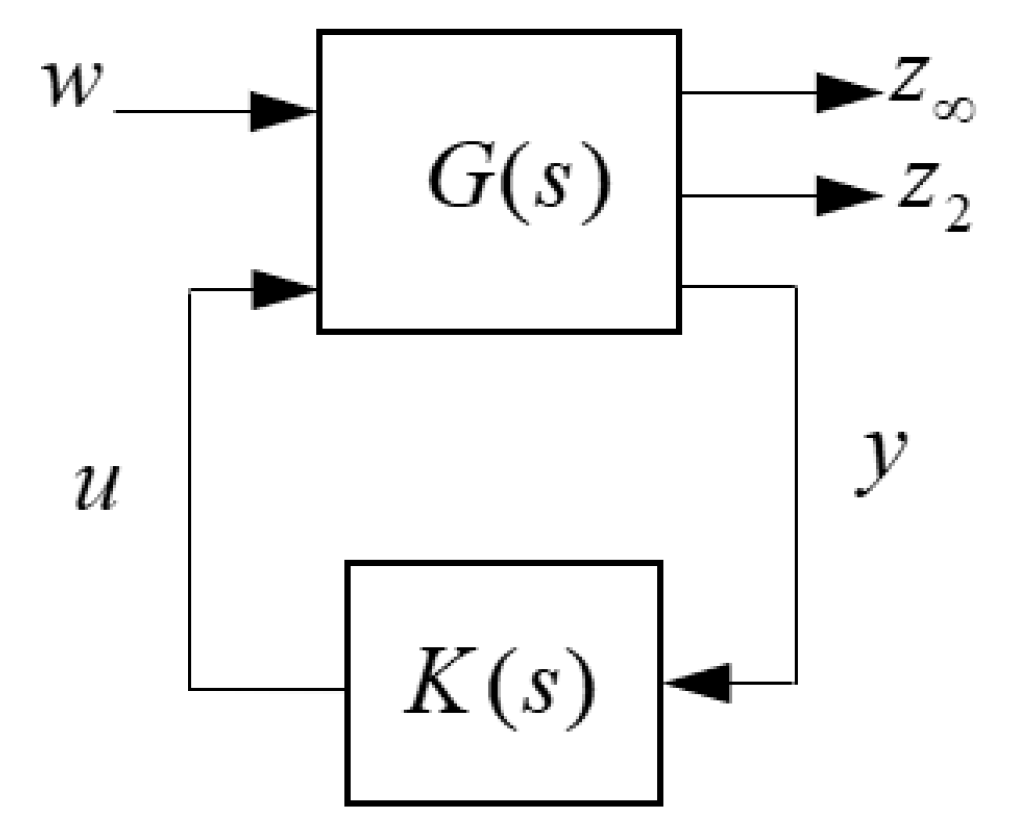
3.1. Multi-Objective H2/H∞ Control
3.2. Controller Design
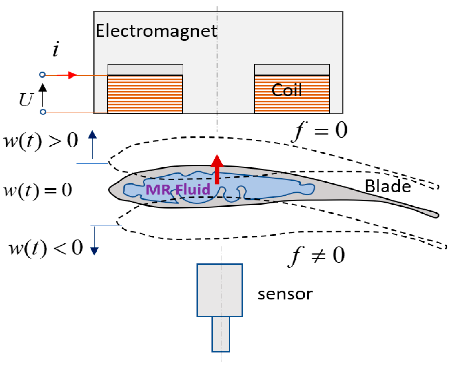
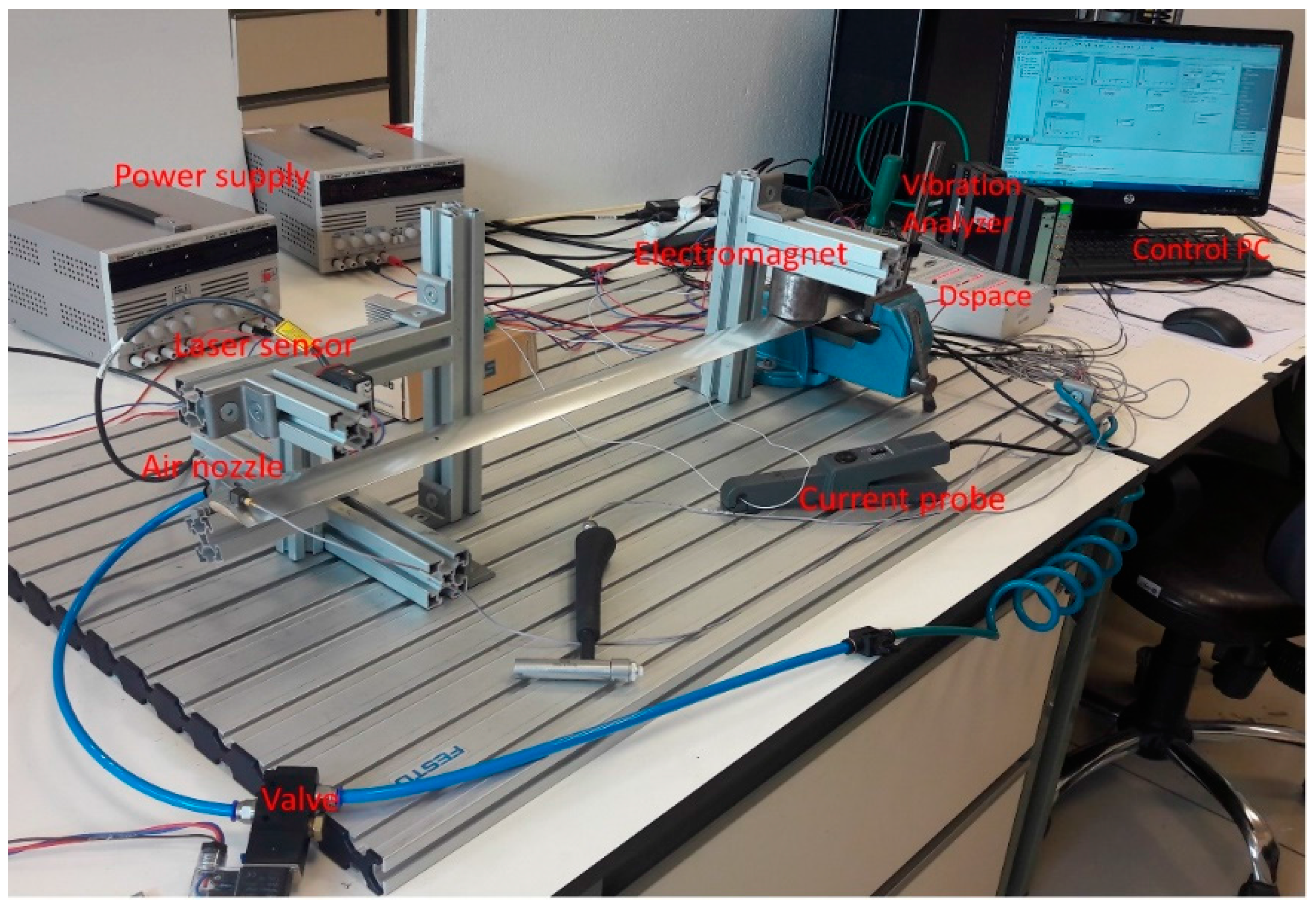
4. Experimental System
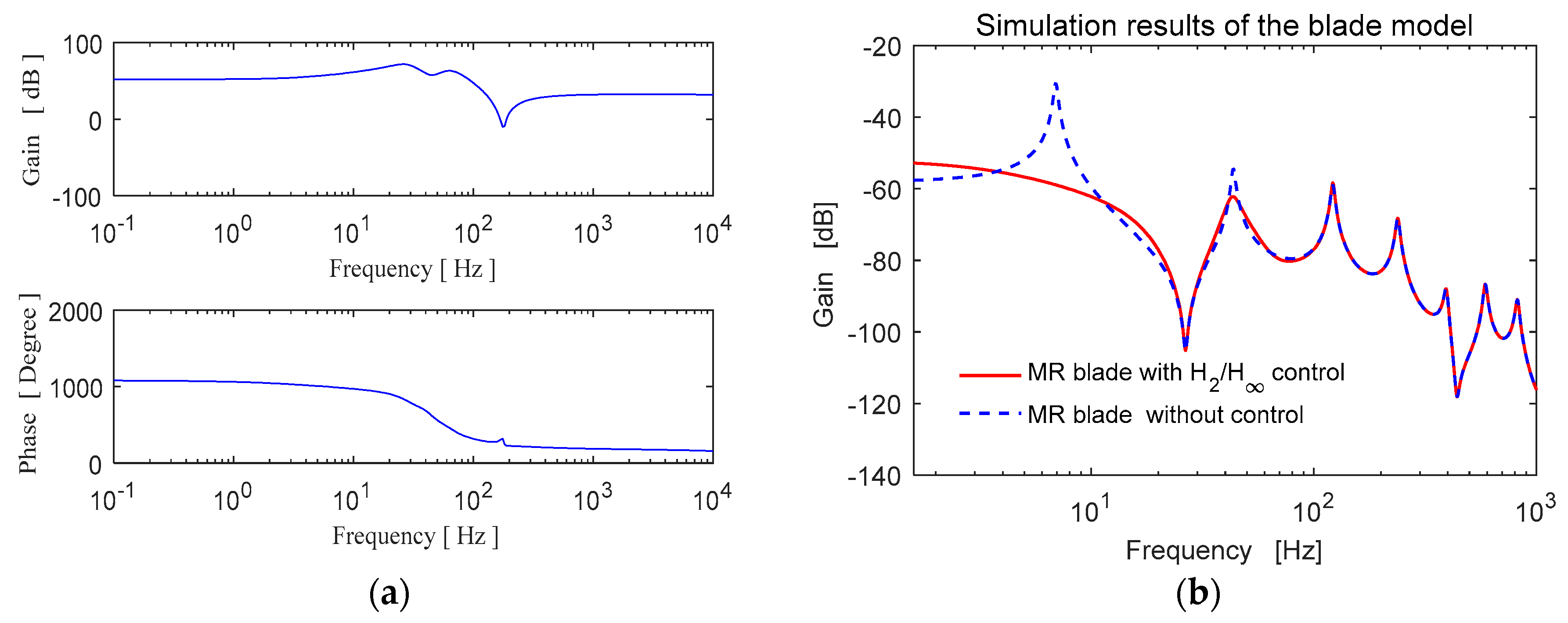
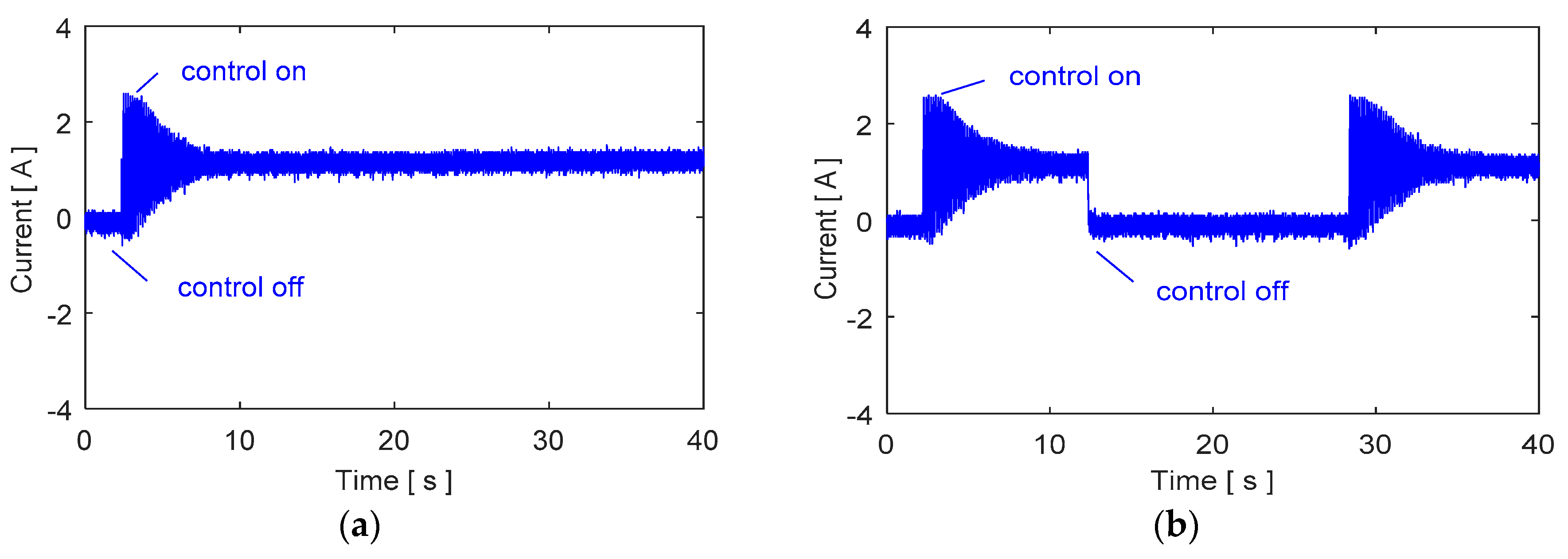
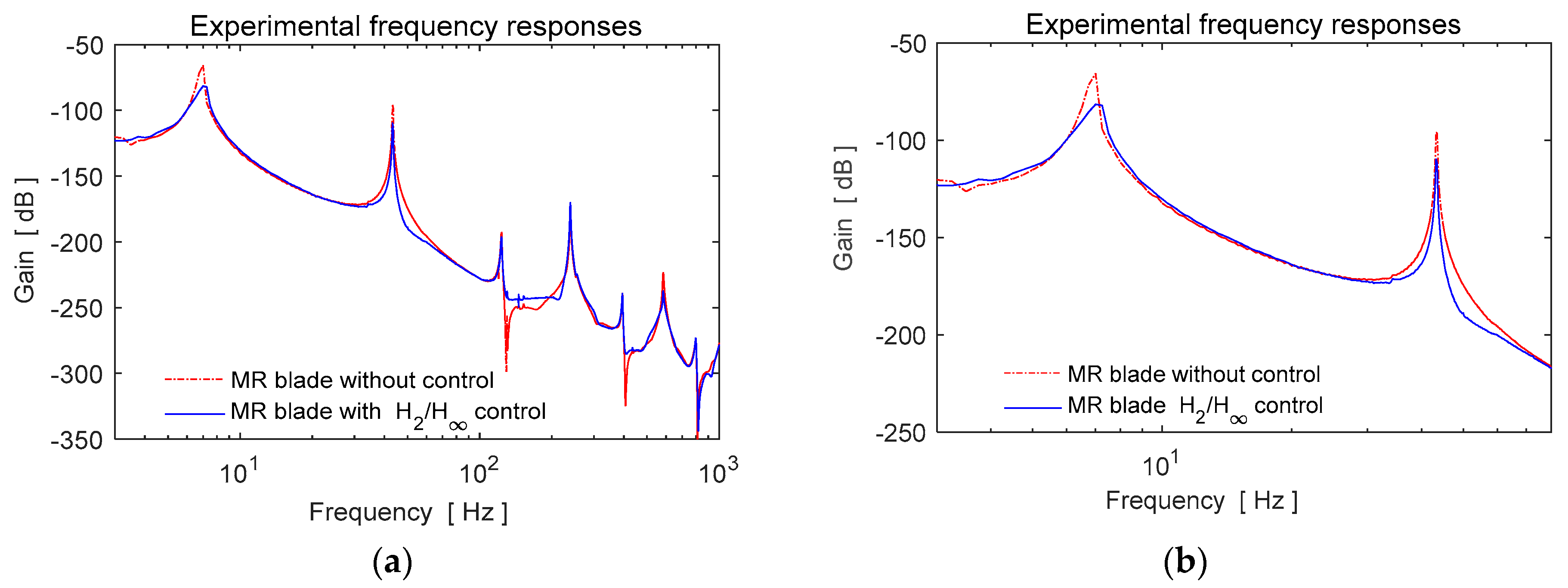
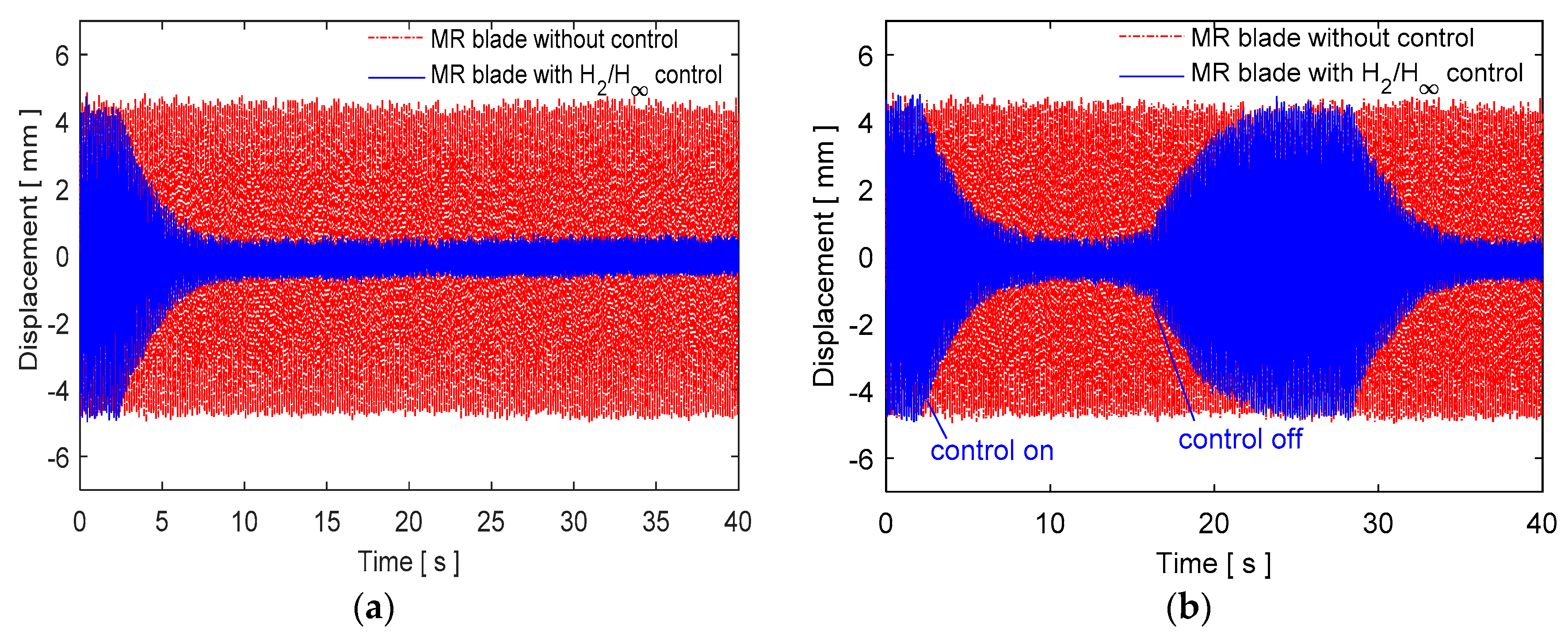
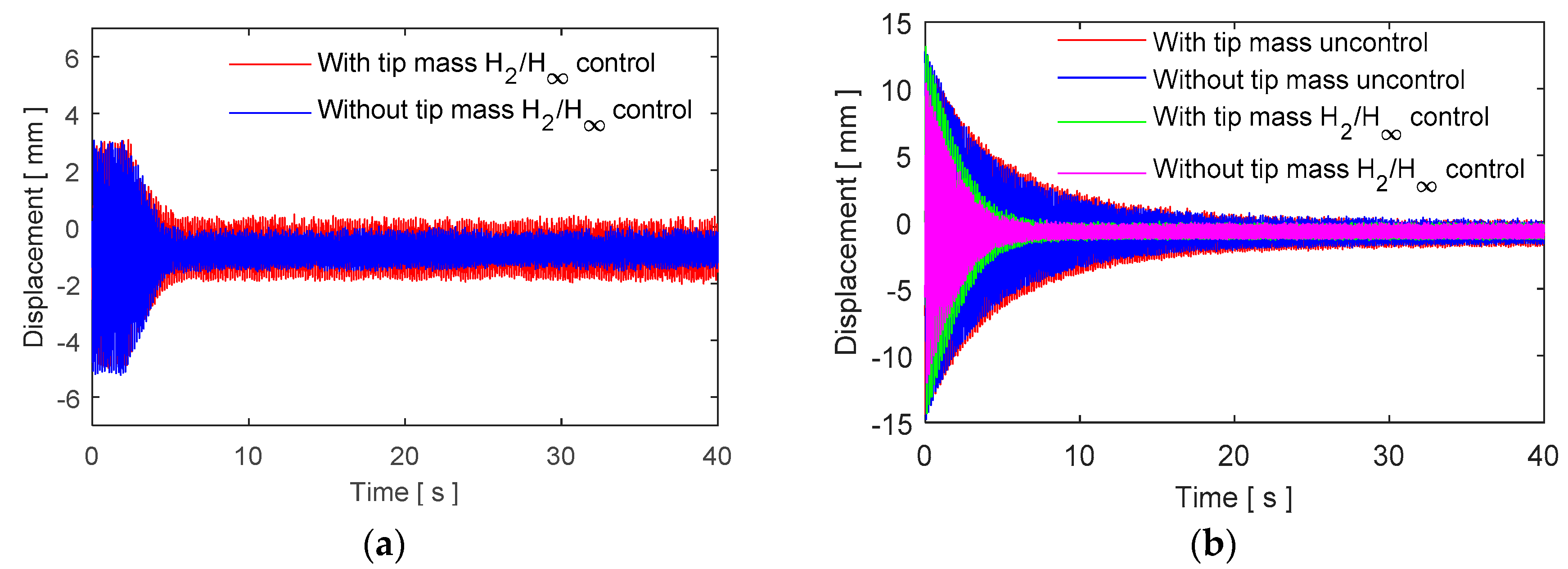
Experimental Results
5. Conclusions
Acknowledgments
Author Contributions
Conflicts of Interest
References
- Sun, Q.; Zhou, J.X.; Zhang, L. An adaptive beam model and dynamic characteristics of magnetorheological materials. J. Sound Vib. 2003, 261, 465–481. [Google Scholar] [CrossRef]
- Yang, G. Large-Scale Magnetorheological Fluid Damper for Vibration Mitigation: Modeling, Testing and Control. Ph.D. Thesis, University of Notre Dame, Notre Dame, IN, USA, 2001. [Google Scholar]
- Yalcintas, M.; Dai, H. Magnetorheological and electrorheological materials in adaptive structures and their performance comparison. Smart Mater. Struct. 1999, 8, 560. [Google Scholar] [CrossRef]
- Spencer, B.F., Jr.; Nagarajaiah, S. State of the art of structural control. J. Struct. Eng. 2003, 129, 845–856. [Google Scholar] [CrossRef]
- Chen, L.; Hansen, C.H. Active vibration control of a magnetorheological sandwich beam. In Proceedings of the Australian Acoustical Society Conference, Busselton, Western Australia, 9–11 November 2005; pp. 93–98. [Google Scholar]
- Xu, Y.L.; Qu, W.L.; Ko, J.M. Seismic response control of frame structures using magnetorheological/electrorheological dampers. Earthq. Eng. Struct. Dyn. 2000, 29, 557–575. [Google Scholar] [CrossRef]
- Stanway, R.; Sproston, J.L.; El Wahed, A.K. Applications of electrorheological fluids in vibration control: A survey. Smart Mater. Struct. 1996, 5, 464–482. [Google Scholar] [CrossRef]
- Niu, H.; Zhang, Y.; Zhang, X.; Xie, S. Active vibration control of plates using electro-magnetic constrained layer damping. Int. J. Appl. Electromagn. Mech. 2010, 33, 831–837. [Google Scholar]
- Valevate, A.V. Semi-Active Vibration Control of a Beam Using Embedded Magneto-Rheological Fluids. Ph.D. Thesis, Wright State University, Dayton, OH, USA, 2004. [Google Scholar]
- Choi, S.B.; Park, Y.K.; Jung, S.B. Modal characteristics of a flexible smart plate filled with electrorheological fluids. J. Air. 1999, 36, 458–464. [Google Scholar] [CrossRef]
- Choi, S.B.; Thompson, B.S.; Gandhi, M.V. Experimental control of a single-link flexible arm incorporating electrorheological fluids. J. Guid. Control Dyn. 1995, 18, 916–919. [Google Scholar] [CrossRef]
- Rajamohan, V.; Sedaghati, R.; Rakheja, S. Optimal vibration control of beams with total and partial MR-fluid treatments. Smart Mater. Struct. 2011, 20, 115016. [Google Scholar] [CrossRef]
- Yeh, J.Y. Vibration analysis of sandwich rectangular plates with magnetorheological elastomer damping treatment. Smart Mater. Struct. 2013, 22, 035010. [Google Scholar] [CrossRef]
- Cortés, F.; Sarría, I. Dynamic analysis of three-layer sandwich beams with thick viscoelastic damping core for finite element applications. Shock Vib. 2015. [Google Scholar] [CrossRef]
- Martin, L.A. A Novel Material Modulus Functions for Modeling Viscoelastic Materials. Ph.D. Thesis, Virginia Polytechnic Institute and State University, Blacksburg, VA, USA, 2011. [Google Scholar]
- Hirunyapruk, C. Vibration Control Using an Adaptive Tuned Magneto-Rheological Fluid Vibration Absorber. Ph.D. Thesis, University of Southampton, Southampton, UK, 2009. [Google Scholar]
- Hu, B.; Wang, D.; Xia, P.; Shi, Q. Investigation on the vibration characteristics of a sandwich beam with smart composites-MRF. World J. Model. Simul. 2006, 2, 201–206. [Google Scholar]
- Kolekar, S.; Venkatesh, K.; Oh, J.S.; Choi, S.B. The tenability of vibration parameters of a sandwich beam featuring controllable core: Experimental Investigation. Adv. Acoust. Vib. 2017. [Google Scholar] [CrossRef]
- Malaeke, H.; Moeenfard, H.; Ghasemi, A.H.; Baqersad, J. Vibration suppression of MR sandwich beams based on fuzzy logic. In Shock & Vibration, Aircraft/Aerospace, Energy Harvesting, Acoustics & Optics; Springer: Cham, Switzerland, 2017; Volume 9, pp. 227–238. [Google Scholar]
- Manoharan, R.; Vasudevan, R.; Sudhagar, P.E. Semi-active vibration control of laminated composite sandwich plate—An experimental study. Arch. Mech. Eng. 2016, 63, 367–377. [Google Scholar] [CrossRef]
- Somers, D.M.; Maughmer, M.D. Theoretical Aerodynamic Analyses of Six Airfoils for Use on Small Wind Turbines; Report No. NREL/SR-500-33295; National Renewable Energy Laboratory: Golden, CO, USA, 2003. [Google Scholar]
- Eshaghi, M.; Rakheja, S.; Sedaghati, R. An accurate technique for pre-yield characterization of MR fluids. Smart Mater. Struct. 2015, 24, 065018. [Google Scholar] [CrossRef]
- Fonseca, H.A.; Gonzalez, E.; Restrepo, J.; Parra, C.A.; Ortiz, C. Magnetic effect in viscosity of magnetorheological fluids. J. Phys. Conf. Ser. 2016, 687, 012102. [Google Scholar] [CrossRef]
- Weiss, K.D.; Carlson, J.D.; Nixon, D.A. Viscoelastic properties of magneto-and electro-rheological fluids. J. Intell. Mater. Syst. Struct. 1994, 5, 772–775. [Google Scholar] [CrossRef]
- Selig, M.S.; McGranahan, B.D. Wind tunnel aerodynamic tests of six airfoils for use on small wind turbines. J. Sol. Energy Eng. (Trans. ASME) 2004, 126, 986–1001. [Google Scholar] [CrossRef]
- Sivrioglu, S.; Nonami, K. Active vibration control by means of LMI-based mixed H2/H∞ state feedback control. JSME Int. J. Ser. C Mech. Syst. Mach. Elem. Manuf. 1997, 40, 239–244. [Google Scholar] [CrossRef]
- Sivrioglu, S.; Tanaka, N.; Yuksek, I. Acoustic power suppression of a panel structure using H-infinity output feedback control. J. Sound Vib. 2002, 249, 885–897. [Google Scholar] [CrossRef]
- Zhou, K.; Doyle, J.C. Essentials of Robust Control; Prentice Hall: Upper Saddle River, NJ, USA, 1997. [Google Scholar]


| Natural Frequencies | Without MR Fluid-Blade Profile Experimental Results [Hz] | Blade Profile Experimental Results [Hz] | Blade Profile ANSYS Results [Hz] | Equivalent Beam Element ANSYS Results [Hz] | Equivalent Beam Analytical Model [Hz] |
|---|---|---|---|---|---|
| 1 | 9.5 | 7 | 7.44 | 7.24 | 7.15 |
| 2 | 59.5 | 43.50 | 46.25 | 45.308 | 44.81 |
| 3 | 167 | 123.5 | 127.12 | 125.74 | 125.48 |
| Mode Number | Gain Reduction [dB] |
|---|---|
| 1.mode | 15.83 |
| 2.mode | 13.07 |
© 2018 by the authors. Licensee MDPI, Basel, Switzerland. This article is an open access article distributed under the terms and conditions of the Creative Commons Attribution (CC BY) license (http://creativecommons.org/licenses/by/4.0/).
Share and Cite
Bolat, F.C.; Sivrioglu, S. Active Control of a Small-Scale Wind Turbine Blade Containing Magnetorheological Fluid. Micromachines 2018, 9, 80. https://doi.org/10.3390/mi9020080
Bolat FC, Sivrioglu S. Active Control of a Small-Scale Wind Turbine Blade Containing Magnetorheological Fluid. Micromachines. 2018; 9(2):80. https://doi.org/10.3390/mi9020080
Chicago/Turabian StyleBolat, Fevzi Cakmak, and Selim Sivrioglu. 2018. "Active Control of a Small-Scale Wind Turbine Blade Containing Magnetorheological Fluid" Micromachines 9, no. 2: 80. https://doi.org/10.3390/mi9020080
APA StyleBolat, F. C., & Sivrioglu, S. (2018). Active Control of a Small-Scale Wind Turbine Blade Containing Magnetorheological Fluid. Micromachines, 9(2), 80. https://doi.org/10.3390/mi9020080