

Stochastic Dynamic Analysis of a Three-Tailed Helical Microrobot in Confined Spaces


Abstract
1. Introduction
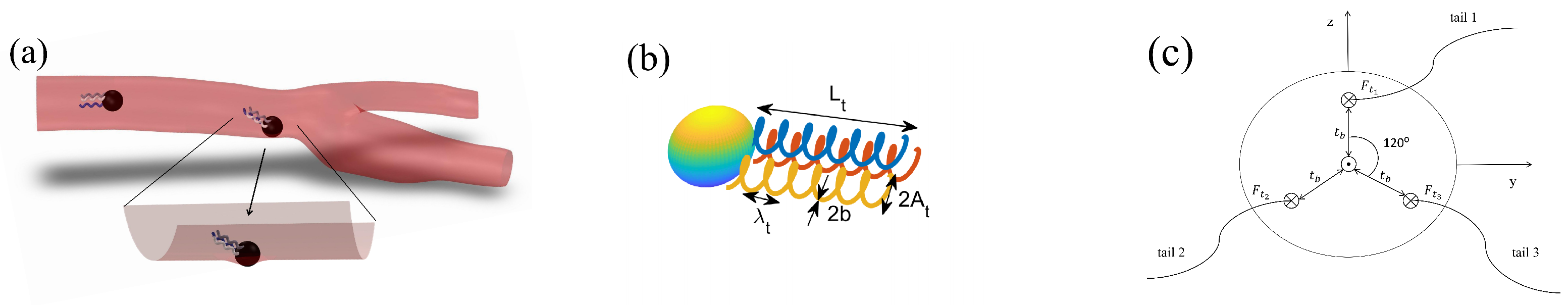
2. Model
3. Simulation Results
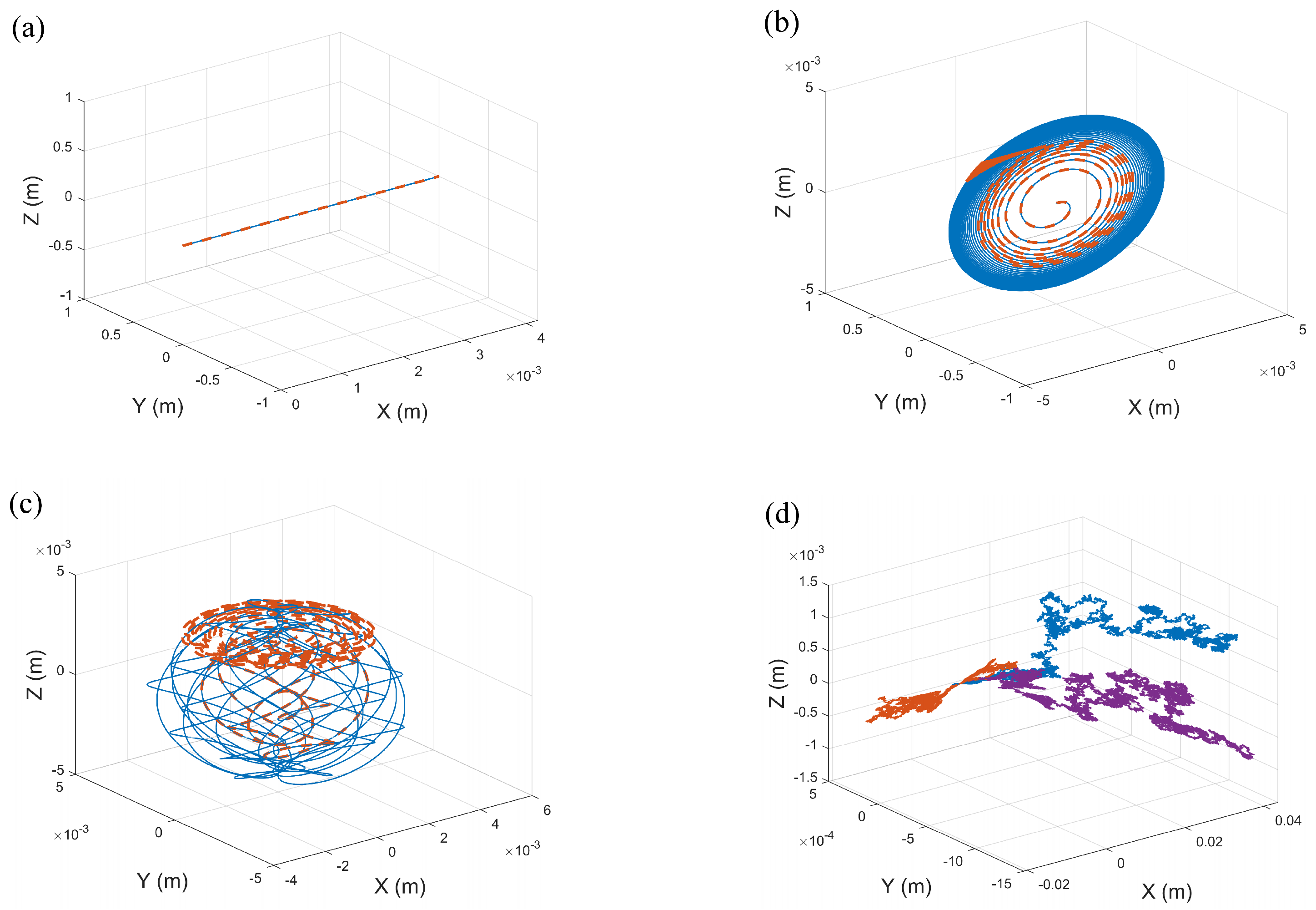
3.1. The Influence on the Trajectory
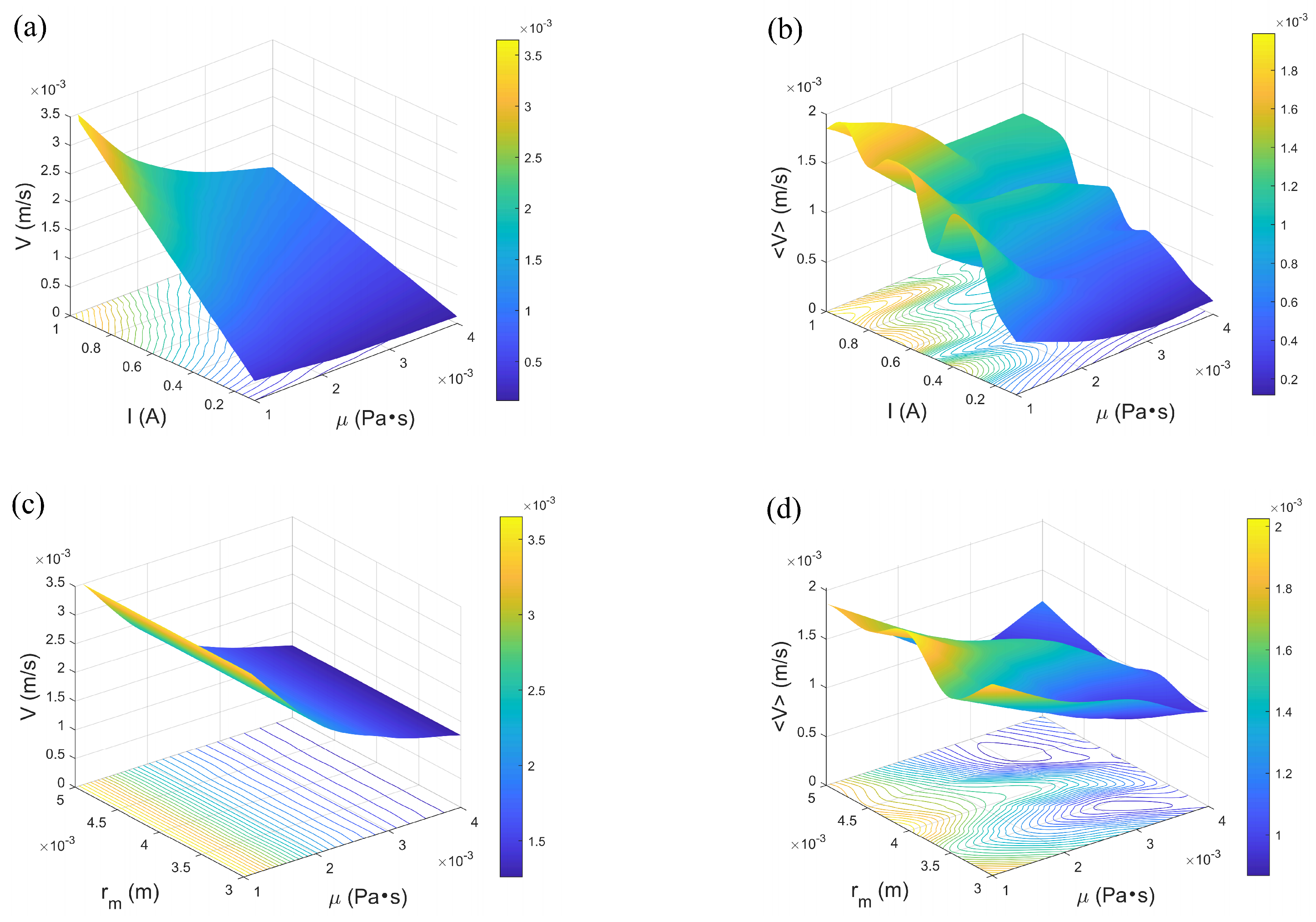
3.2. The Influence on the Velocity
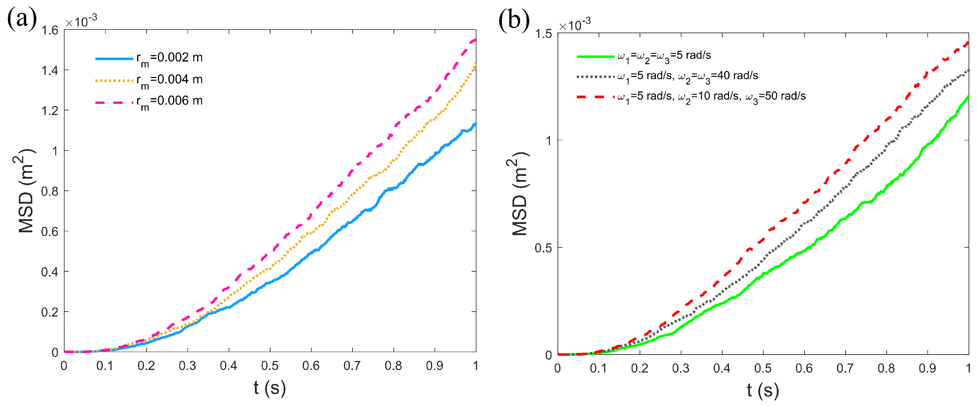
3.3. The Mean Squared Displacement
3.4. The Wobbling Rate
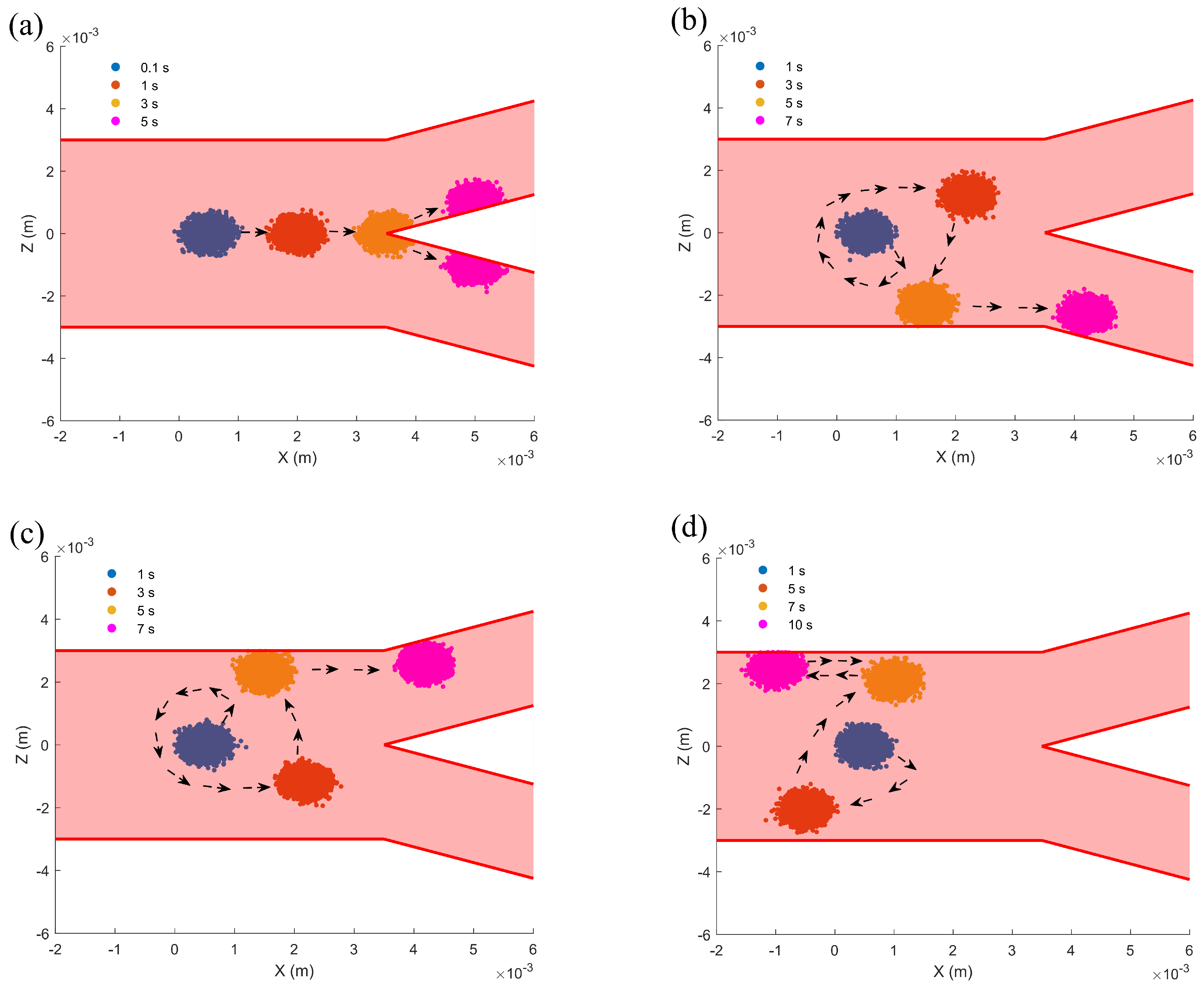
3.5. Motion Trajectory in Bifurcated Channels
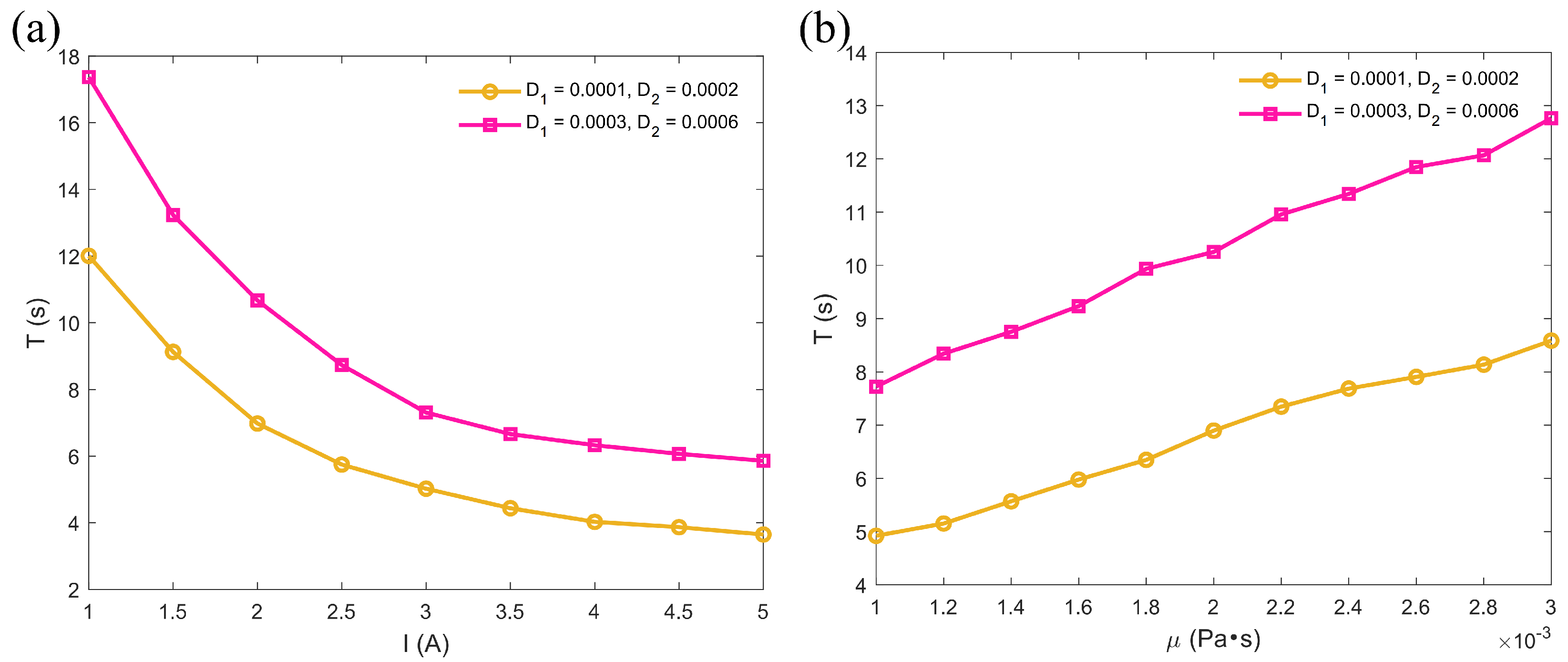
3.6. The Time to Reach the Bifurcation
4. Conclusions
Author Contributions
Funding
Data Availability Statement
Acknowledgments
Conflicts of Interest
References
- Lee, J.G.; Raj, R.R.; Day, N.B.; Shields IV, C.W. Microrobots for biomedicine: Unsolved challenges and opportunities for translation. ACS Nano 2023, 17, 14196–14204. [Google Scholar] [PubMed]
- Zheng, Z.; Wang, H.; Dong, L.; Shi, Q.; Li, J.; Sun, T.; Huang, Q.; Fukuda, T. Ionic shape-morphing microrobotic end-effectors for environmentally adaptive targeting, releasing, and sampling. Nat. Commun. 2021, 12, 411. [Google Scholar] [PubMed]
- Shui, L.; Ni, K.; Wang, Z. Aligned magnetic nanocomposites for modularized and recyclable soft microrobots. Acs Appl. Mater. Interfaces 2022, 14, 43802–43814. [Google Scholar] [PubMed]
- Nguyen, K.T.; Go, G.; Jin, Z.; Darmawan, B.A.; Yoo, A.; Kim, S.; Nan, M.; Lee, S.B.; Kang, B.; Kim, C.S.; et al. A magnetically guided self-rolled microrobot for targeted drug delivery, real-time X-Ray imaging, and microrobot retrieval. Adv. Healthc. Mater. 2021, 10, 2001681. [Google Scholar]
- Zhang, S.; Scott, E.Y.; Singh, J.; Chen, Y.; Zhang, Y.; Elsayed, M.; Chamberlain, M.D.; Shakiba, N.; Adams, K.; Yu, S.; et al. The optoelectronic microrobot: A versatile toolbox for micromanipulation. Proc. Natl. Acad. Sci. USA 2019, 116, 14823–14828. [Google Scholar]
- Cappelleri, D.J.; Piazza, G.; Kumar, V. A two dimensional vision-based force sensor for microrobotic applications. Sensors Actuators Phys. 2011, 171, 340–351. [Google Scholar]
- Yang, L.; Zhang, L. Motion control in magnetic microrobotics: From individual and multiple robots to swarms. Annu. Rev. Control. Robot. Auton. Syst. 2021, 4, 509–534. [Google Scholar]
- Yang, L.; Sun, M.; Zhang, M.; Zhang, L. Multimodal motion control of soft ferrofluid robot with environment and task adaptability. IEEE/Asme Trans. Mechatronics 2023, 28, 3099–3109. [Google Scholar]
- Xin, C.; Jin, D.; Hu, Y.; Yang, L.; Li, R.; Wang, L.; Ren, Z.; Wang, D.; Ji, S.; Hu, K.; et al. Environmentally adaptive shape-morphing microrobots for localized cancer cell treatment. ACS Nano 2021, 15, 18048–18059. [Google Scholar]
- Shi, X.; Li, Y.; Xu, Y.; Liu, Q. Complex dynamics of a magnetic microrobot driven by single deformation soft tail in random environment. Theor. Appl. Mech. Lett. 2024, 14, 100534. [Google Scholar]
- Williams, B.J.; Anand, S.V.; Rajagopalan, J.; Saif, M.T.A. A self-propelled biohybrid swimmer at low Reynolds number. Nat. Commun. 2014, 5, 3081. [Google Scholar] [PubMed]
- Khalil, I.S.; Tabak, A.F.; Hamed, Y.; Tawakol, M.; Klingner, A.; El Gohary, N.; Mizaikoff, B.; Sitti, M. Independent actuation of two-tailed microrobots. IEEE Robot. Autom. Lett. 2018, 3, 1703–1710. [Google Scholar]
- Khalil, I.S.; Klingner, A.; Hamed, Y.; Hassan, Y.S.; Misra, S. Controlled noncontact manipulation of nonmagnetic untethered microbeads orbiting two-tailed soft microrobot. IEEE Trans. Robot. 2020, 36, 1320–1332. [Google Scholar]
- Xing, J.; Ning, C.; Zhi, Y.; Howard, I. Analysis of bifurcation and chaotic behavior of the micro piezoelectric pipe-line robot drive system with stick-slip mechanism. Commun. Nonlinear Sci. Numer. Simul. 2024, 134, 107998. [Google Scholar]
- Wang, G.; Bickerdike, A.; Liu, Y.; Ferreira, A. Analytical solution of a microrobot-blood vessel interaction model. Nonlinear Dyn. 2025, 113, 2091–2109. [Google Scholar]
- Lu, K.; Zhou, C.; Li, Z.; Liu, Y.; Wang, F.; Xuan, L.; Wang, X. Multi-level magnetic microrobot delivery strategy within a hierarchical vascularized organ-on-a-chip. Lab Chip 2024, 24, 446–459. [Google Scholar]
- Yang, L.; Wang, Q.; Zhang, L. Model-free trajectory tracking control of two-particle magnetic microrobot. IEEE Trans. Nanotechnol. 2018, 17, 697–700. [Google Scholar]
- Liu, Z.; Qin, F.; Zhu, L.; Yang, R.; Luo, X. Effects of the intrinsic curvature of elastic filaments on the propulsion of a flagellated microrobot. Phys. Fluids 2020, 32, 041902. [Google Scholar]
- Temel, F.Z.; Yesilyurt, S. Simulation-based analysis of micro-robots swimming at the center and near the wall of circular mini-channels. Microfluid. Nanofluidics 2013, 14, 287–298. [Google Scholar]
- Aghakhani, A.; Yasa, O.; Wrede, P.; Sitti, M. Acoustically powered surface-slipping mobile microrobots. Proc. Natl. Acad. Sci. USA 2020, 117, 3469–3477. [Google Scholar]
- Fan, X.; Sun, M.; Sun, L.; Xie, H. Ferrofluid droplets as liquid microrobots with multiple deformabilities. Adv. Funct. Mater. 2020, 30, 2000138. [Google Scholar]
- Su, M.; Xu, T.; Lai, Z.; Huang, C.; Liu, J.; Wu, X. Double-modal locomotion and application of soft cruciform thin-film microrobot. IEEE Robot. Autom. Lett. 2020, 5, 806–812. [Google Scholar]
- Chattopadhyay, S.; Moldovan, R.; Yeung, C.; Wu, X. Swimming efficiency of bacterium Escherichia coli. Proc. Natl. Acad. Sci. USA 2006, 103, 13712–13717. [Google Scholar]
- Patil, G.; Ghosh, A. Analysing the motion of scallop-like swimmers in a noisy environment. Eur. Phys. J. Spec. Top. 2023, 232, 927–933. [Google Scholar] [PubMed]
- Ghosh, A.; Paria, D.; Rangarajan, G.; Ghosh, A. Velocity fluctuations in helical propulsion: How small can a propeller be. J. Phys. Chem. Lett. 2014, 5, 62–68. [Google Scholar]
- Ryan, P.; Diller, E. Magnetic actuation for full dexterity microrobotic control using rotating permanent magnets. IEEE Trans. Robot. 2017, 33, 1398–1409. [Google Scholar]
- Boudaoud, M.; Haddab, Y.; Le Gorrec, Y.; Lutz, P. Noise characterization in millimeter sized micromanipulation systems. Mechatronics 2011, 21, 1087–1097. [Google Scholar]
- Berman, S.A.; Mitchell, K.A. Swimmer dynamics in externally driven fluid flows: The role of noise. Phys. Rev. Fluids 2022, 7, 014501. [Google Scholar]
- Meng, K.; Jia, Y.; Yang, H.; Niu, F.; Wang, Y.; Sun, D. Motion planning and robust control for the endovascular navigation of a microrobot. IEEE Trans. Ind. Informatics 2019, 16, 4557–4566. [Google Scholar]
- Peyer, K.E.; Tottori, S.; Qiu, F.; Zhang, L.; Nelson, B.J. Magnetic helical micromachines. Chem. Eur. J. 2013, 19, 28–38. [Google Scholar]
- Arcese, L.; Fruchard, M.; Ferreira, A. Endovascular magnetically guided robots: Navigation modeling and optimization. IEEE Trans. Biomed. Eng. 2011, 59, 977–987. [Google Scholar] [PubMed]
- Fier, G.; Hansmann, D.; Buceta, R.C. Langevin equations for the run-and-tumble of swimming bacteria. Soft Matter 2018, 14, 3945–3954. [Google Scholar] [PubMed]
- Acemoglu, A.; Yesilyurt, S. Effects of geometric parameters on swimming of micro organisms with single helical flagellum in circular channels. Biophys. J. 2014, 106, 1537–1547. [Google Scholar] [PubMed]


| Parameter Name | Symbol | Value |
|---|---|---|
| Radius of the magnetic sphere | r | |
| Length of the tail | ||
| Amplitude of the tail | ||
| Wavelength of the tail | ||
| Maximum wall deformation | ||
| Permanent deformation | ||
| Offset distance | ||
| Mean radius of the coil | R | |
| Cross-sectional radius of the tail | b | |
| Coil turn | n | |
| Poisson’s ratio of the microrobot | ||
| Poisson’s ratio of the blood vessel wall | ||
| Young’s modulus of the microrobot | ||
| Young’s modulus of the blood vessel wall | ||
| Density of the sphere | ||
| Density of the tail | ||
| Permeability of free space | ||
| Magnetization | M |
Disclaimer/Publisher’s Note: The statements, opinions and data contained in all publications are solely those of the individual author(s) and contributor(s) and not of MDPI and/or the editor(s). MDPI and/or the editor(s) disclaim responsibility for any injury to people or property resulting from any ideas, methods, instructions or products referred to in the content. |
© 2025 by the authors. Licensee MDPI, Basel, Switzerland. This article is an open access article distributed under the terms and conditions of the Creative Commons Attribution (CC BY) license (https://creativecommons.org/licenses/by/4.0/).
Share and Cite
Shi, X.; Li, Y.; Suleiman, K. Stochastic Dynamic Analysis of a Three-Tailed Helical Microrobot in Confined Spaces. Micromachines 2025, 16, 373. https://doi.org/10.3390/mi16040373
Shi X, Li Y, Suleiman K. Stochastic Dynamic Analysis of a Three-Tailed Helical Microrobot in Confined Spaces. Micromachines. 2025; 16(4):373. https://doi.org/10.3390/mi16040373
Chicago/Turabian StyleShi, Xinpeng, Yongge Li, and Kheder Suleiman. 2025. "Stochastic Dynamic Analysis of a Three-Tailed Helical Microrobot in Confined Spaces" Micromachines 16, no. 4: 373. https://doi.org/10.3390/mi16040373
APA StyleShi, X., Li, Y., & Suleiman, K. (2025). Stochastic Dynamic Analysis of a Three-Tailed Helical Microrobot in Confined Spaces. Micromachines, 16(4), 373. https://doi.org/10.3390/mi16040373