4.1. Prominent Local Maxima for Object Localization
To verify the hypothesis that the proposed minimal “redundant count map” tends to generate a prominent local maximum at each target center, we extract the pixel value of each predicted target and its proportion in a square kernel in the predicted location map. Experimental results of prominent local maxima for each dataset are summarized in
Table 2. The kernel size
r was supposed to cover 99.7% of instances following a normalized Gaussian distribution, i.e.,
. Therefore, the Gaussian center in
Table 2 represents the central response of a normalized Gaussian distribution with a standard deviation of
. It is found that although the mean local maximum and its mean proportion over the kernel in the predicted location maps decrease as the target/kernel size increases, they are still higher than the Gaussian center by a large margin (greater than three times), especially for Honeybee, Fish, MBM, and ST Part B datasets.
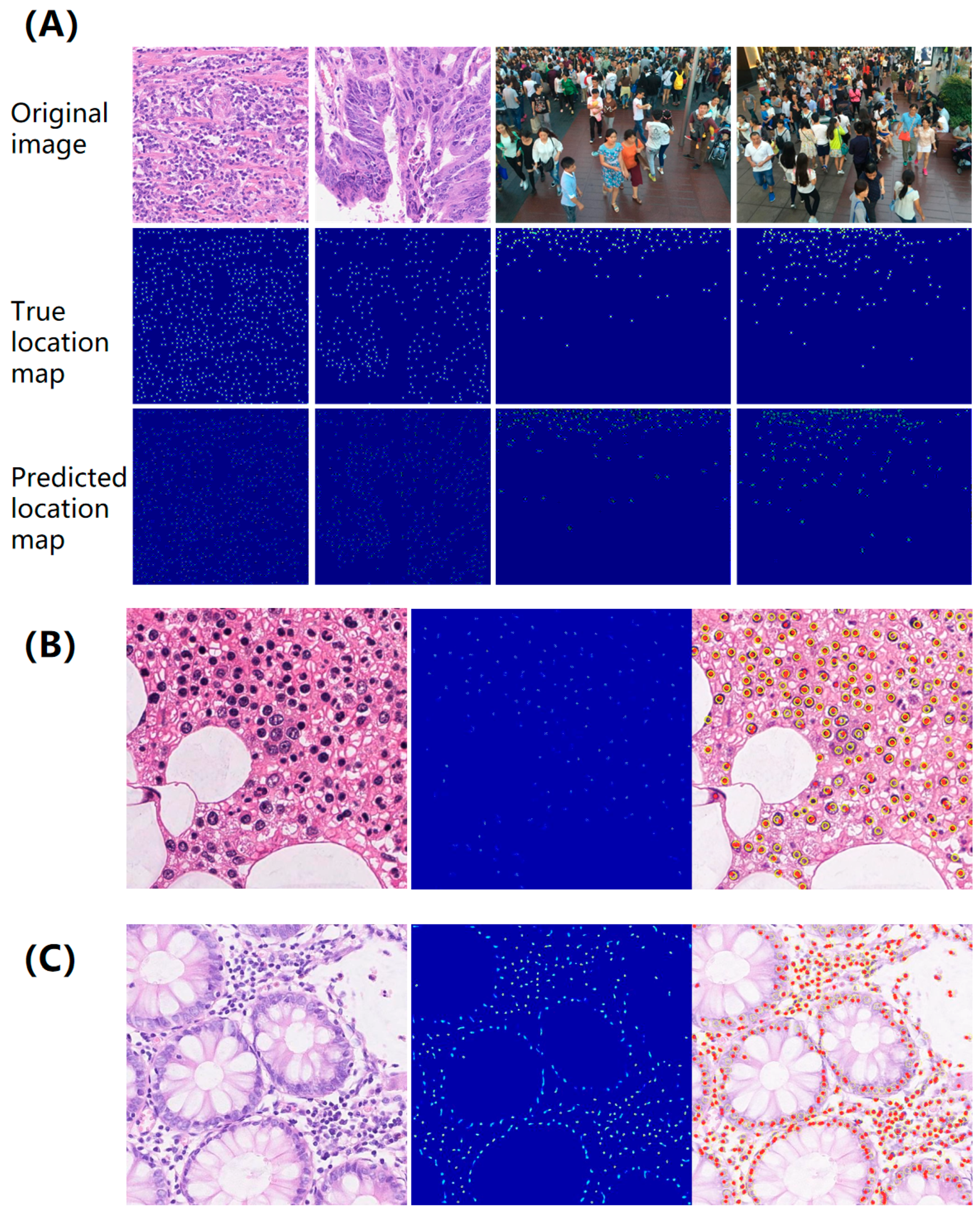
The results of the true and the predicted location map are presented in
Figure 4, which illustrates typical examples of location maps in instance-dense regions. It is observed that each target is visually independent even in dense crowds, indicating the effectiveness of the proposed map in handling incomplete annotations. In addition, a key advantage of this method is its tendency to yield prominent local maxima at the centers of targets, serving as reliable markers for localizing small objects (see
Supplementary Figure S2). Additionally, the uniqueness of the proposed solution to the minimization problem is separately validated through a theoretical derivation provided in
Supplementary Note S5. It ensures that our model converges to a single, plausible estimate of the underlying object locations. This property, enhanced by our well-conditioned transformation, makes the learning process inherently robust to noise and ambiguities in the training annotations. In conclusion, the proposed minimal “redundant count map” is evaluated for localized instances with incomplete annotations and a tendency toward prominent local maxima at the object center.
4.2. Performance Comparison Between Baseline and the Proposed Method
We further quantify the localization performance of the proposed approach and compare it with baseline methods. Experimental results on each test dataset are shown in
Table 3,
Table 4,
Table 5,
Table 6 and
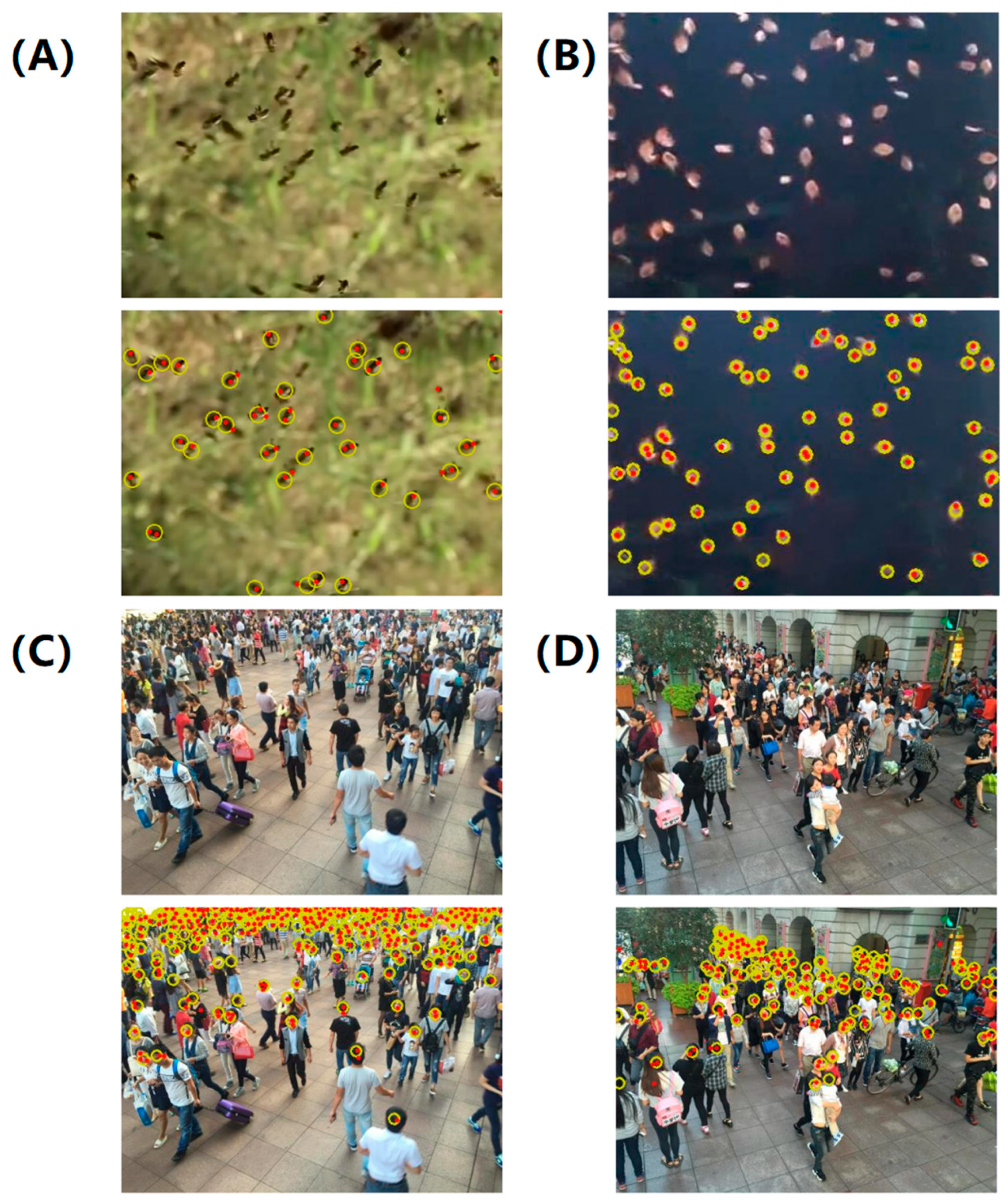
Table 7 with a varying number of point annotations, in which LFE represents our proposed approach, and the following digits represent the number of point annotations employed in the training process. For example, LFE-3 indicates that only three annotations were provided in each image for training LFE. The percentage of labels in the last column also shows the proportion of partially annotated examples. The bold black font indicates the best performance, and the blue font highlights the performance of the proposed LFE supervised by approximately 10% of all annotation points. The representative visualization of localization results supervised by less than 10% of point annotations is also shown in
Figure 5.
CA cells dataset. Table 3 provides a comparison of the proposed approach’s localization performance against other sophisticated methods, including SSAE [
31], SR-CNN [
21], SC-CNN [
1], SFCN-OPI [
16], SSL-LIR, and WSL-LIR [
17], on the CA cell test dataset. The results indicate that our LFE method utilizing 100 and 50 labeled examples achieves comparable performance to fully supervised SC-CNN and SR-CNN approaches, despite being supervised by only 33.7% and 16.8% of the annotated points, respectively. Furthermore, when compared to our previous weakly supervised WSL-LIR [
17], the LFE-50 can reduce annotation costs by more than 50%, while maintaining an almost identical F1 score. It is also concluded that the PU learning strategy with unsupervised loss modeling can successfully learn to localize small instances from a few point annotation examples.
Table 3.
The localization performance on the CA cells dataset.
Table 3.
The localization performance on the CA cells dataset.
| Method | Precision | Recall | F1 Score ↑ | Labels |
|---|
| SSAE | 0.617 | 0.644 | 0.630 | 0% |
| SR-CNN | 0.783 | 0.804 | 0.793 | 100% |
| SC-CNN | 0.781 | 0.823 | 0.802 | 100% |
| SFCN-OPI | 0.819 | 0.874 | 0.834 | 100% |
| SSL-LIR | 0.854 | 0.850 | 0.852 | 100% |
| WSL-LIR | 0.810 | 0.777 | 0.793 | 43.8% |
| LFE-100 | 0.78 ± 0.02 | 0.83 ± 0.02 | 0.80 ± 0.01 | 33.7% |
| LFE-50 | 0.76 ± 0.02 | 0.82 ± 0.01 | 0.79 ± 0.01 | 16.8% |
| LFE-25 | 0.75 ± 0.02 | 0.81 ± 0.02 | 0.78 ± 0.01 | 8.4% |
| LFE-10 | 0.74 ± 0.02 | 0.75 ± 0.04 | 0.74 ± 0.02 | 3.4% |
Interestingly, when the label reduction is increased by more than 91.6%, the F1 score of the LFE-25 is only 0.023 lower than that of the LFE-100, indicating that our approach is not overly sensitive to label reduction. Even with a further reduction in labeled examples, the LFE-10 (adopting only 3.4% labels) still outperforms the unsupervised SSAE approach by a considerable margin. A distinctive advantage of LFE over unsupervised and fully supervised methodology is its ability to exploit data scarcity. In scenarios where a minute portion (<10%) of the data is labeled, LFE can optimize the existing information by focusing on the most enlightening examples. This strategy can potentially lead to more precise forecasting and enhanced generalization capabilities.
MBM cells dataset. Table 4 exhibits the performance quantification of our approach at different levels of label reduction on histopathological bone marrow images. Exploiting less than 39.7% of annotated points, the LFE-50 network achieves comparable localization performance with the fully supervised SSL-LIR approach [
17]. In addition, when less than 8% of labeled examples are utilized for training, the LFE-10 can still precisely localize more than 83% of the targets in the test dataset, suggesting its effectiveness. The LFE framework offers several potential benefits over fully supervised approaches (detailed in
Supplementary Note S6), while a key benefit is that it allows for a more efficient use of labeled data.
Table 4.
The localization performance on the MBM cells dataset.
Table 4.
The localization performance on the MBM cells dataset.
| Method | Precision | Recall | F1 Score ↑ | Labels % |
|---|
| SSL-LIR | 0.885 | 0.873 | 0.879 | 100% |
| LFE-50 | 0.83 ± 0.02 | 0.90 ± 0.02 | 0.87 ± 0.01 | 39.7% |
| LFE-25 | 0.81 ± 0.02 | 0.88 ± 0.01 | 0.84 ± 0.01 | 19.8% |
| LFE-10 | 0.76 ± 0.01 | 0.83 ± 0.04 | 0.79 ± 0.01 | 7.9% |
| LFE-5 | 0.75 ± 0.03 | 0.76 ± 0.03 | 0.75 ± 0.02 | 4.0% |
Honeybee and Fish datasets. Compared to the SIDIP method [
10], the LFE-15 model achieves the same localization performance on the Honeybee test dataset, as shown in
Table 5, while requiring only 53.6% of labeled points. Because the number of honeybees in each image is relatively small, 90% label reduction means fewer than three targets in an image have been annotated. In this situation, our LFE-3 algorithm still successfully detected about 83% of the small honeybees in the test dataset, while 72% of the location predictions suggest true positives, proving the feasibility of small object localization with 90% annotation reduction.
Table 5.
The localization performance on the Honeybee dataset.
Table 5.
The localization performance on the Honeybee dataset.
| Method | Precision | Recall | F1 Score ↑ | Labels |
|---|
| SIDIP | 0.921 | 0.787 | 0.849 | 100% |
| LFE-15 | 0.79 ± 0.04 | 0.91 ± 0.03 | 0.85 ± 0.03 | 53.6% |
| LFE-10 | 0.78 ± 0.04 | 0.91 ± 0.03 | 0.84 ± 0.03 | 35.7% |
| LFE-5 | 0.68 ± 0.06 | 0.86 ± 0.04 | 0.76 ± 0.03 | 17.9% |
| LFE-3 | 0.72 ± 0.11 | 0.83 ± 0.04 | 0.76 ± 0.05 | 10.7% |
Comparative localization performance on the Fish dataset was also demonstrated in
Table 6. It was observed that even though less than 20% of labeled targets were provided for the training stage, our LFE-10 approach still outperforms the fully supervised SIDIP method. In addition, the localization performance of the LFE-5 with 91.1% label reduction is very close to that of SIDIP using 100% annotations. To further demonstrate the effectiveness of the proposed LFE-10 algorithm, we conducted a series of experiments on both datasets. The results are shown in
Figure 5A,B, showing that nearly all of the small objects are captured and localized. The LFE-10 algorithm achieves an average localization error of 2 pixels, which is better than the fully supervised SIDIP method. The LFE-10 algorithm also achieved a higher precision and recall rate of 96% and 94% compared to the SIDIP method.
Table 6.
The localization performance on the Fish dataset.
Table 6.
The localization performance on the Fish dataset.
| Method | Precision | Recall | F1 Score ↑ | Labels |
|---|
| SIDIP | 0.951 | 0.921 | 0.936 | 100% |
| LFE-25 | 0.97 ± 0.01 | 0.95 ± 0.01 | 0.96 ± 0.01 | 44.6% |
| LFE-15 | 0.95 ± 0.02 | 0.95 ± 0.01 | 0.95 ± 0.01 | 26.8% |
| LFE-10 | 0.96 ± 0.01 | 0.94 ± 0.02 | 0.95 ± 0.01 | 17.9% |
| LFE-5 | 0.94 ± 0.03 | 0.90 ± 0.05 | 0.92 ± 0.04 | 8.9% |
ST Part B. A detailed study of the ST Part B dataset of human crowds shows that the proposed LFE method outperforms other state-of-the-art methods in the MLE metric. The performance comparison on the ST Part B dataset is exhibited in
Table 7, where LS-CNN and CSR-A-thr results are directly from the literature [
41]. The proposed LFE supervised by 82.3% of point annotations outperforms the fully supervised LSC-CNN method. Encouragingly, even though only 10% of the point annotations (12 examples) are randomly selected to supervise our training procedure, the average localization error is still lower than that of CSR-A-thr by a large margin. A representative visualization of the localization results was shown in
Supplementary Figure S3, suggesting that our method would not deteriorate significantly with the decreasing number of annotation examples. The ability of the proposed method to handle complex data structures and large datasets makes it a superior choice for localization tasks of small objects.
Table 7.
The localization performance on the ST Part B dataset.
Table 7.
The localization performance on the ST Part B dataset.
| Method | MLE ↓ | Labels |
|---|
| CSR-A-thr | 12.28 | 100% |
| LSC-CNN | 9.0 | 100% |
| LFE-100 | 8.70 ± 0.14 | 81.3% |
| LFE-50 | 9.63 ± 0.21 | 40.6% |
| LFE-25 | 10.10 ± 0.24 | 20.3% |
| LFE-12 | 10.79 ± 0.43 | 9.8% |
4.3. Ablation Study on Pseudo-Labeling
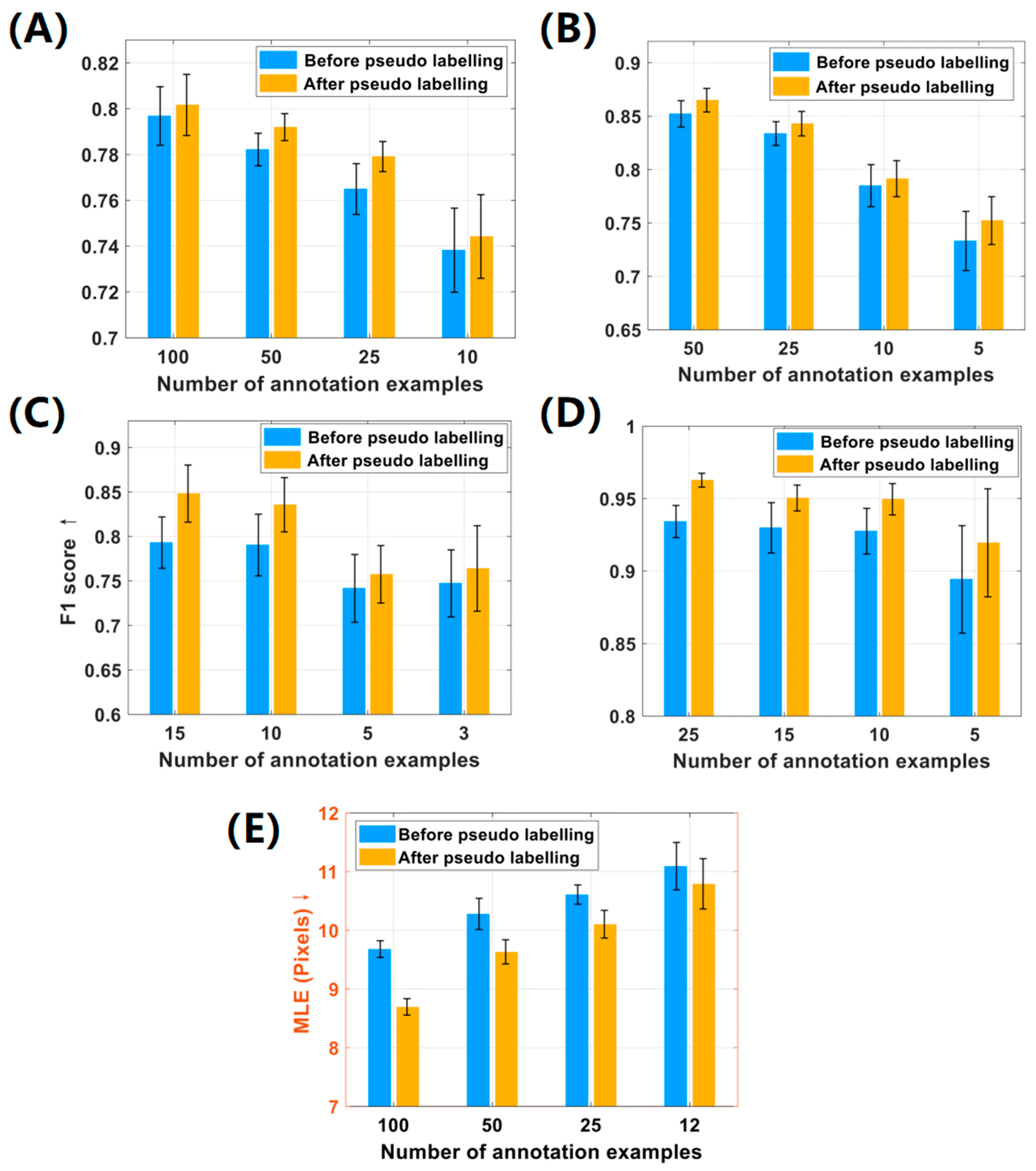
To demonstrate the effectiveness of the pseudo-labeling strategy in the LFE method, we recorded and analyzed the localization performance before and after the pseudo-labeling process. The experimental results are depicted in
Figure 6. It is notable that the implementation of pseudo-labeling boosted the overall F1 score of localization by 0.5%~5% in the first four datasets. Specifically, in the Honeybee and Fish datasets, the average performance after pseudo-labeling was notably improved by 3.32% and 2.41%, respectively. In the CA and MBM cell datasets, significant improvements in F1 scores were also noted in different numbers of point annotations.
Similarly, the pseudo-labeling process in the ST Part B dataset significantly reduced the mean localization error MLE by 5.9%. Objectively speaking, the efficiency of the LFE method can deteriorate with the reduction of labeled examples due to the decline in supervised information. This is because algorithms rely on the abundance of data to generalize and make accurate predictions. Without sufficient examples, most algorithms may not be able to fully capture the variations and complexity in the data. However,
Figure 6 indicates that the LFE method performs remarkably well on the Fish dataset, even with a label reduction of more than 90%. This is attributed to the fact that the small objects in this dataset share similar morphological features, which are less susceptible to the perspective changes. Furthermore, it is evident from
Figure 6 that the standard deviation (black error bar) of the F1 score increases with the reduction of labels, because fewer labeled examples are less likely to cover all visual features of targets compared to a majority of annotations. In summary, our method demonstrated consistent performance across all datasets, showing notable improvement in localization performance after pseudo-labeling. In addition, our method is robust for label reduction, as it can effectively handle datasets with more than 90% unlabeled examples.
