
Numerical Simulation of the Photobleaching Process in Laser-Induced Fluorescence Photobleaching Anemometer


Abstract
:1. Introduction
2. LIFPA Photobleaching Model
3. Experimental Setup
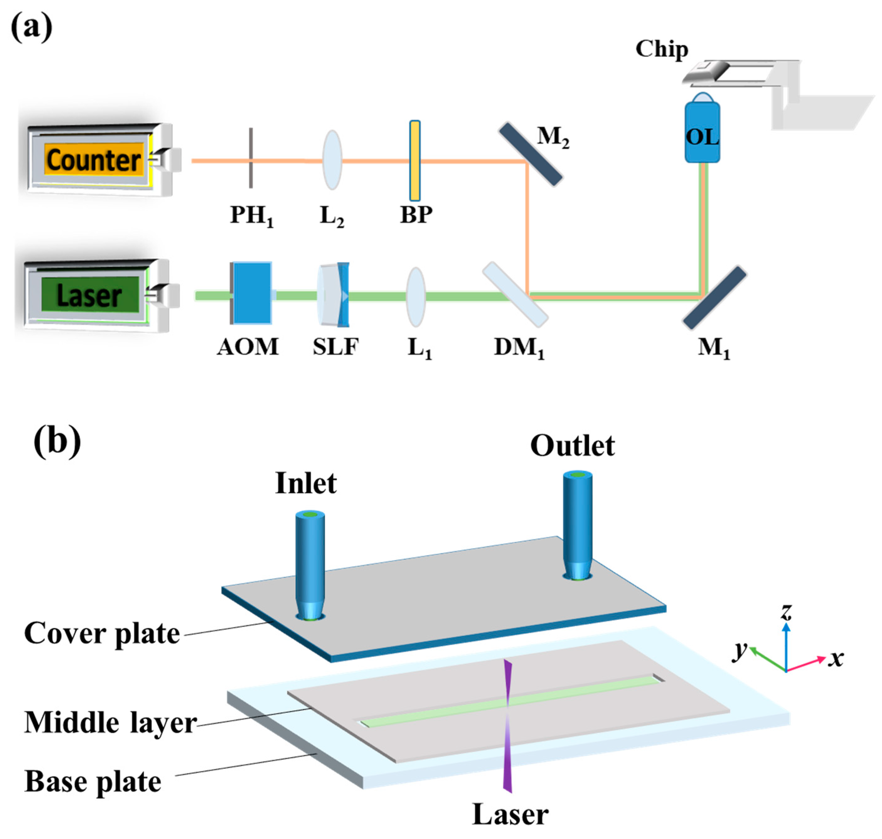
3.1. LIFPA System
3.2. Microchannel and Solution Preparation
4. Numerical Simulation and Experiment
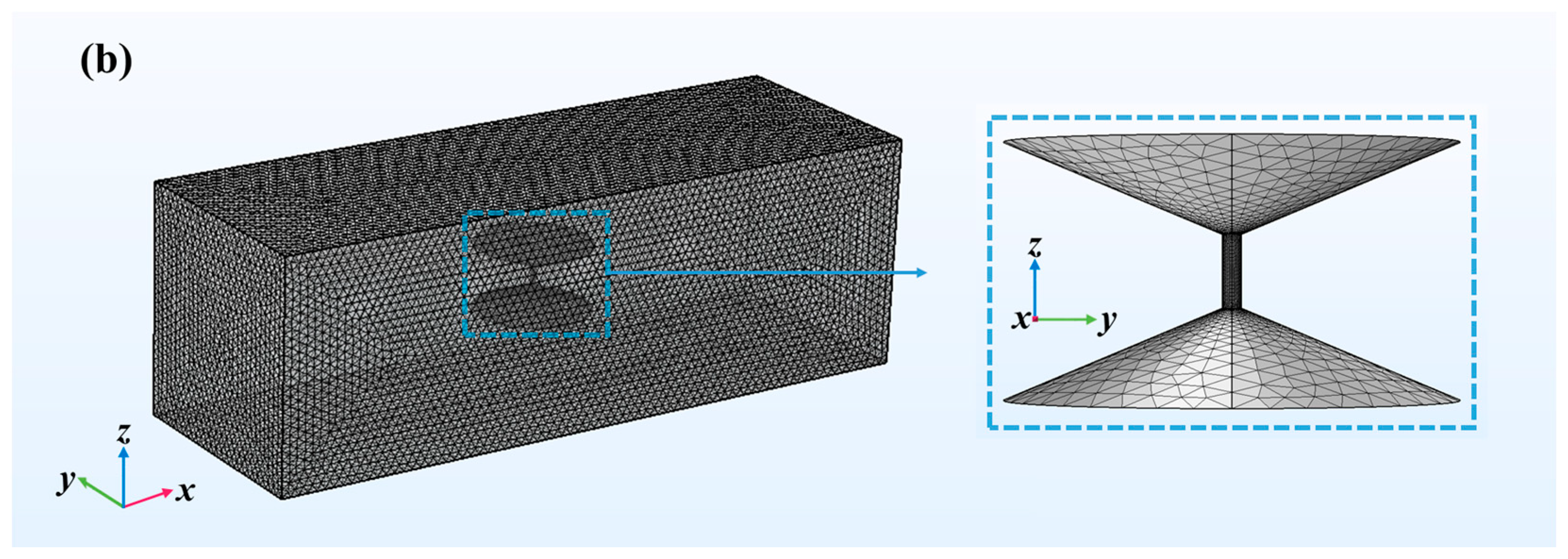
4.1. Numerical Simulation by COMSOL
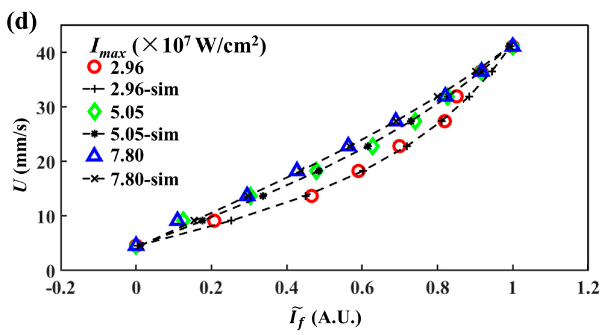
4.2. Direct Comparison between Experiments and Numerical Simulations
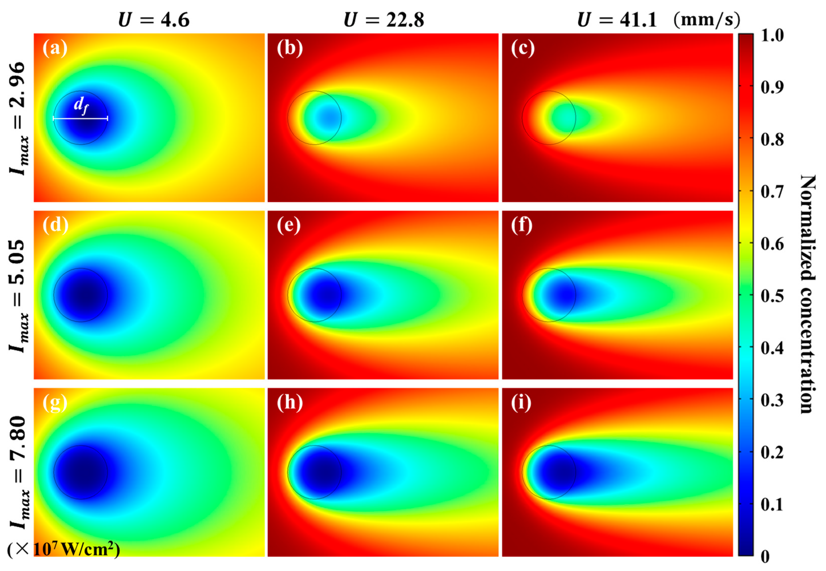
4.3. Effective Concentration Distribution
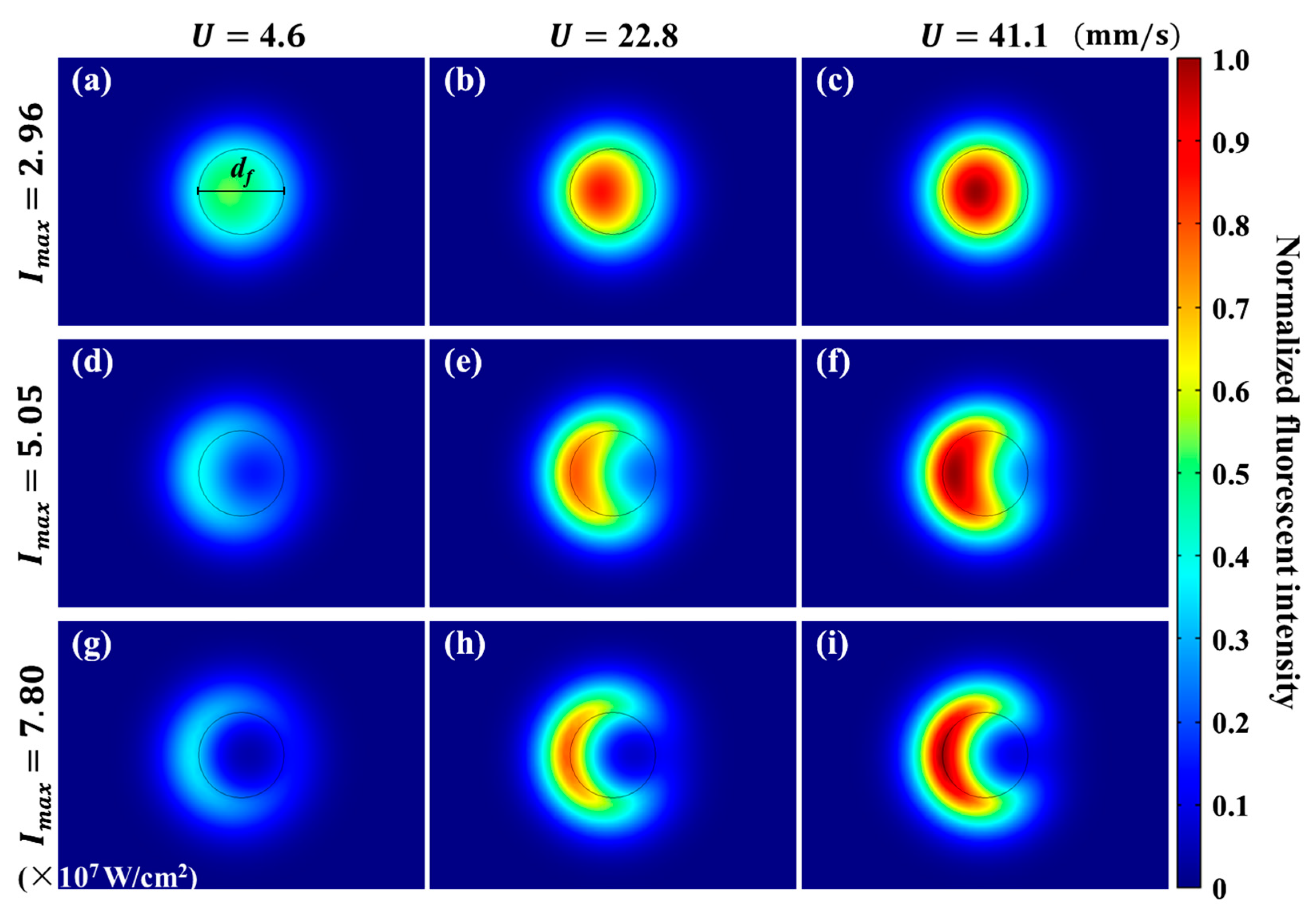
4.4. Fluorescence Intensity Distribution
5. Velocity Measurement of Breaking Optical Diffraction Limit
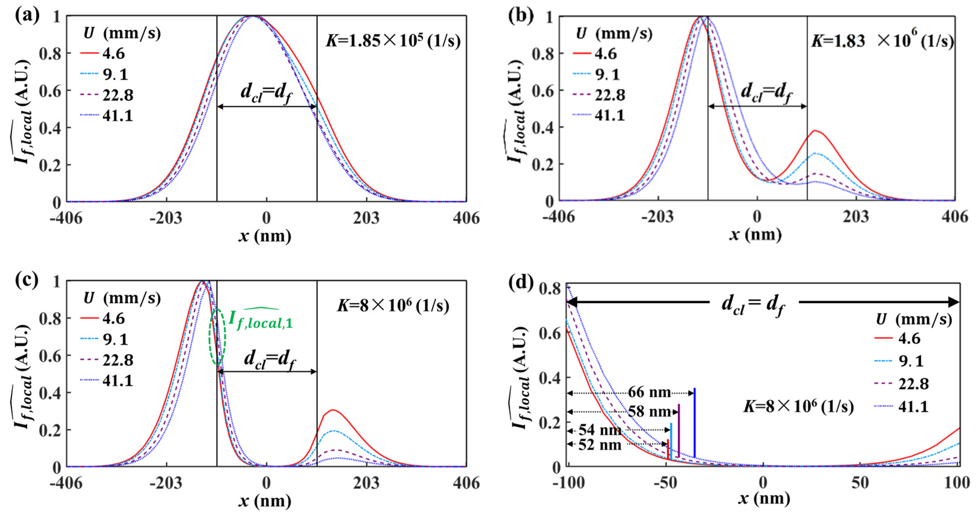
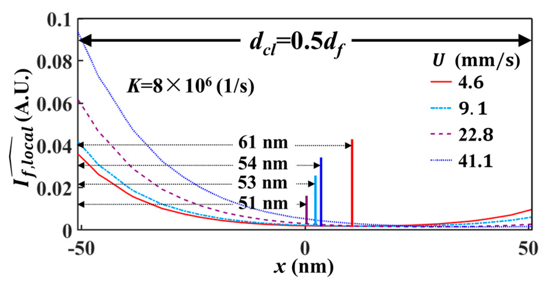
5.1. Spatial Resolution of Effective Velocity Measurement with LIFPA
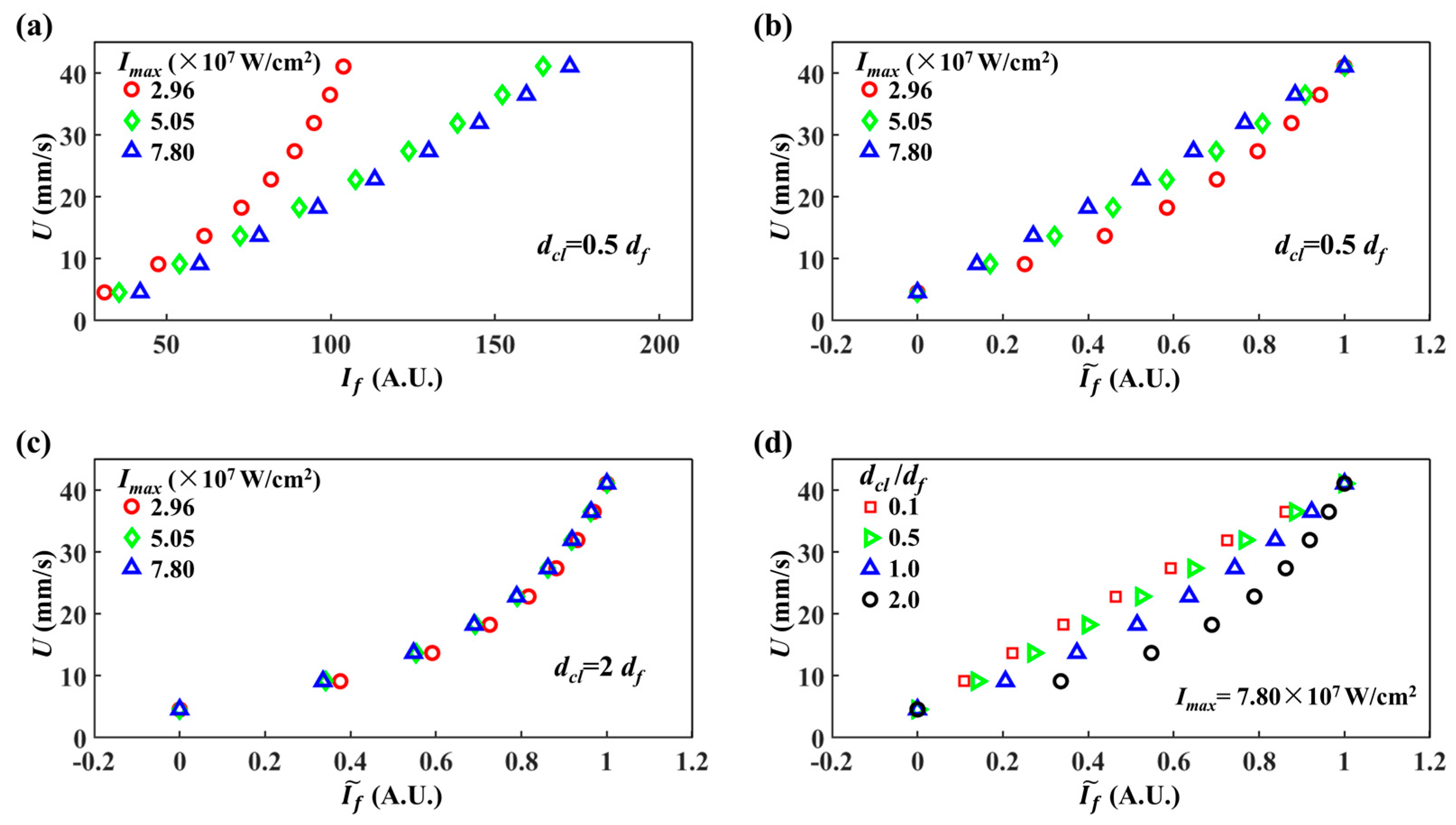
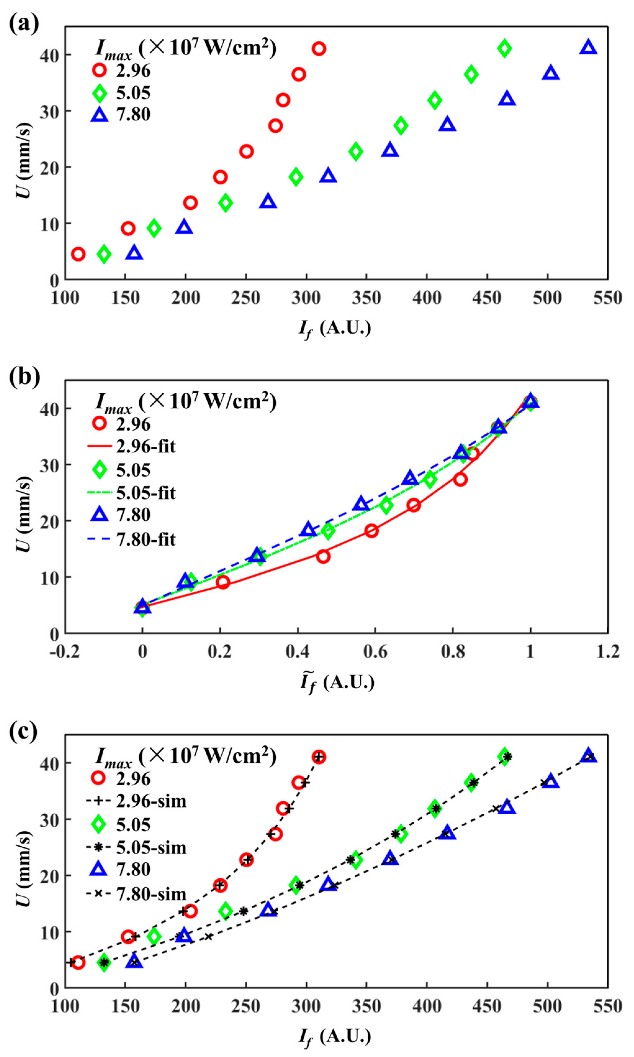
5.2. Influence of Integration Region on Velocity Measurement
6. Conclusions
Author Contributions
Funding
Acknowledgments
Conflicts of Interest
References
- Wang, G.R. Laser induced fluorescence photobleaching anemometer for microfluidic devices. Lab Chip 2005, 5, 450–456. [Google Scholar] [CrossRef] [Green Version]
- Wang, Y.C.; Zhao, W.X.; Hu, Z.Y.; Zhang, C.; Feng, X.Q.; Zhao, W.; Wang, G.R.; Wang, K.G. Parametric study of the emission spectra and photobleaching time constants of a fluorescent dye in laser induced fluorescence photobleaching anemometer (LIFPA) applications. Exp. Fluids 2019, 60, 106. [Google Scholar] [CrossRef]
- Hoebe, R.A.; van Der Voort, H.T.M.; Stap, J.; van Noorden, C.J.F.; Manders, E.M.M. Quantitative determination of the reduction of phototoxicity and photobleaching by controlled light exposure microscopy. J. Microsc. 2008, 231, 9–20. [Google Scholar] [CrossRef]
- Kuang, C.F.; Yang, F.; Zhao, W.; Wang, G.R. Study of the Rise Time in Electroosmotic Flow within a Microcapillary. Anal. Chem. 2009, 81, 6590–6595. [Google Scholar] [CrossRef]
- Zhao, W.; Yang, F.; Khan, J.; Reifsnider, K.; Wang, G.R. Corrections on LIFPA velocity measurements in microchannel with moderate velocity fluctuations. Exp. Fluids 2015, 56, 39. [Google Scholar] [CrossRef]
- Kuang, C.F.; Wang, G.R. A novel far-field nanoscopic velocimetry for nanofluidics. Lab Chip 2010, 10, 240–245. [Google Scholar] [CrossRef] [Green Version]
- Kuang, C.F.; Qiao, R.; Wang, G.R. Ultrafast measurement of transient electroosmotic flow in microfluidics. Microfluid. Nanofluidics 2011, 11, 353–358. [Google Scholar] [CrossRef]
- Zhao, W.; Liu, X.; Yang, F.; Wang, K.G.; Bai, J.T.; Qiao, R.; Wang, G.R. Study of Oscillating Electroosmotic Flows with High Temporal and Spatial Resolution. Anal. Chem. 2018, 90, 1652–1659. [Google Scholar] [CrossRef]
- Hu, Z.Y.; Zhao, T.Y.; Wang, H.X.; Zhao, W.; Wang, K.G.; Bai, J.T.; Wang, G.R. Asymmetric temporal variation of oscillating AC electroosmosis with a steady pressure-driven flow. Exp. Fluids 2020, 61, 233. [Google Scholar] [CrossRef]
- Hu, Z.Y.; Zhao, T.Y.; Zhao, W.; Yang, F.; Wang, H.X.; Wang, K.G.; Bai, J.T.; Wang, G.R. Transition from periodic to chaotic AC electroosmotic flows near electric double layer. AIChE J. 2021, 67, 17148. [Google Scholar] [CrossRef]
- Wang, G.R.; Yang, F.; Zhao, W. There can be turbulence in microfluidics at low Reynolds number. Lab Chip 2014, 14, 1452–1458. [Google Scholar] [CrossRef] [Green Version]
- Wang, G.R.; Yang, F.; Zhao, W. Microelectrokinetic turbulence in microfluidics at low Reynolds number. Phys. Rev. E 2016, 93, 013106. [Google Scholar] [CrossRef] [PubMed] [Green Version]
- Zhao, W.; Yang, F.; Wang, K.G.; Bai, J.T.; Wang, G.R. Rapid mixing by turbulent-like electrokinetic microflow. Chem. Eng. Sci. 2017, 165, 113–121. [Google Scholar] [CrossRef]
- Zhao, W.; Wang, G.R. Scaling of velocity and scalar structure functions in ac electrokinetic turbulence. Phys. Rev. E 2017, 95, 023111. [Google Scholar] [CrossRef] [PubMed] [Green Version]
- Wang, G.R.; Yang, F.; Zhao, W.; Chen, C.P. On micro-electrokinetic scalar turbulence in microfluidics at a low Reynolds number. Lab Chip 2016, 16, 1030–1038. [Google Scholar] [CrossRef]
- Zhao, W.; Yang, F.; Khan, J.; Reifsnider, K.; Wang, G.R. Measurement of velocity fluctuations in microfluidics with simultaneously ultrahigh spatial and temporal resolution. Exp. Fluids 2016, 57, 11. [Google Scholar] [CrossRef]
- Brizitskii, R.V.; Saritskaya, Z.Y. Boundary value and extremal problems for the nonlinear convection-diffusion-reaction equation. J. Alloy. Compd. 2015, 463, 559–563. [Google Scholar]
- Lazarov, R.D.; Tomov, S.Z. Adaptive Finite Volume Element Method for Convection-Diffusion-Reaction Problems in 3-D; Nova Science Publishers, Inc.: Hauppauge, NY, USA, 2000. [Google Scholar]
- Phongthanapanich, S.; Dechaumphai, P. A characteristic-based finite volume element method for convection-diffusion-reaction equation. Trans. Can. Soc. Mech. Eng. 2008, 32, 549–559. [Google Scholar] [CrossRef]
- Taneja, S.; Rutenberg, A.D. Photobleaching of randomly rotating fluorescently decorated particles. J. Chem. Phys. 2017, 147, 104105. [Google Scholar] [CrossRef]
- Gavrilyuk, S.; Polyutov, S.; Jha, P.C.; Rinkevicius, Z.; Ågren, H.; Gel’Mukhanov, F. Many-Photon Dynamics of Photobleaching. J. Phys. Chem. A 2007, 111, 11961–11975. [Google Scholar] [CrossRef]
- Hintschich, S.I.; Rothe, C.; King, S.M.; Clark, S.; Monkman, A.P. The Complex Excited-state Behavior of a Polyspirobifluorene Derivative: The Role of Spiroconjugation and Mixed Charge Transfer Character on Excited-state Stabilization and Radiative Lifetime. J. Phys. Chem. B 2008, 112, 16300–16306. [Google Scholar] [CrossRef] [PubMed]
- Ehrlich, K.; Kufcsák, A.; Krstajić, N.; Henderson, R.K.; Thomson, R.R.; Tanner, M.G. Fibre optic time-resolved spectroscopy using CMOS-SPAD arrays. In Proceedings of the Optical Fibers and Sensors for Medical Diagnostics and Treatment Applications XVII, San Francisco, CA, USA, 28–29 January 2017; International Society for Optics and Photonics: Bellingham, WA, USA, 2017. [Google Scholar]
- Lee, Y.U.; Li, S.L.; Bopp, S.E.; Zhao, J.X.; Nie, Z.Y.; Posner, C.; Yang, S.; Zhang, X.; Zhang, J.; Liu, Z.W. Unprecedented Fluorophore Photostability Enabled by Low-Loss Organic Hyperbolic Materials. Adv. Mater. 2021, 33, 2006496. [Google Scholar] [CrossRef] [PubMed]
- Wang, G.R.; Fiedler, H.E. On High Spatial Resolution Scalar Measurement With LIF. Exp. Fluids 2000, 29, 265–274. [Google Scholar] [CrossRef]
- Lai, M.J.; Pan, R.H.; Zhao, K. Initial Boundary Value Problem for Two-Dimensional Viscous Boussinesq Equations. Arch. Ration. Mech. Anal. 2011, 199, 739–760. [Google Scholar] [CrossRef]
- Verschaeve, J.C.G. Analysis of the lattice Boltzmann Bhatnagar-Gross-Krook no-slip boundary condition: Ways to improve accuracy and stability. Phys. Rev. E 2009, 80, 036703. [Google Scholar] [CrossRef]
- Smistrup, K.; Bu, M.; Wolff, A.; Bruus, H.; Hansen, M.F. Theoretical analysis of a new, efficient microfluidic magnetic bead separator based on magnetic structures on multiple length scales. Microfluid. Nanofluidics. 2008, 4, 565–573. [Google Scholar] [CrossRef]
- Mortensen, N.A.; Okkels, F.; Bruus, H. Reexamination of Hagen-Poiseuille flow: Shape dependence of the hydraulic resistance in microchannels. Phys. Rev. E 2005, 71, 057301. [Google Scholar] [CrossRef] [Green Version]


|
Flow Rate in experiments (μL/min) | 5.0 | 10.0 | 15.0 | 20.0 | 25.0 | 30.0 | 35.0 | 40.0 | 45.0 |
|
Flow rate in simulation (nL/min) | 13.1 | 26.1 | 39.2 | 52.2 | 65.3 | 78.3 | 91.4 | 104.5 | 117.5 |
|
for both experiments and simulations (mm/s) | 4.6 | 9.1 | 13.7 | 18.2 | 22.8 | 27.4 | 31.9 | 36.5 | 41.1 |
| (mW) | 6.90 | 1.80 | 18.20 |
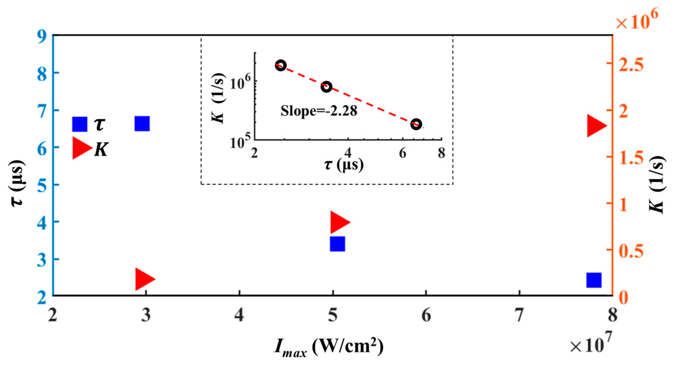
| (W/cm2) | 2.96 × 10⁷ | 5.05 × 10⁷ | 7.80 × 10⁷ |
| (μs) | 6.63 | 3.41 | 2.43 |
| (1/s) | 1.85 × 10⁵ | 7.95 × 10⁵ | 1.83 × 10⁶ |
Publisher’s Note: MDPI stays neutral with regard to jurisdictional claims in published maps and institutional affiliations. |
© 2021 by the authors. Licensee MDPI, Basel, Switzerland. This article is an open access article distributed under the terms and conditions of the Creative Commons Attribution (CC BY) license (https://creativecommons.org/licenses/by/4.0/).
Share and Cite
Chen, Y.; Meng, S.; Wang, K.; Bai, J.; Zhao, W. Numerical Simulation of the Photobleaching Process in Laser-Induced Fluorescence Photobleaching Anemometer. Micromachines 2021, 12, 1592. https://doi.org/10.3390/mi12121592
Chen Y, Meng S, Wang K, Bai J, Zhao W. Numerical Simulation of the Photobleaching Process in Laser-Induced Fluorescence Photobleaching Anemometer. Micromachines. 2021; 12(12):1592. https://doi.org/10.3390/mi12121592
Chicago/Turabian StyleChen, Yu, Shuangshuang Meng, Kaige Wang, Jintao Bai, and Wei Zhao. 2021. "Numerical Simulation of the Photobleaching Process in Laser-Induced Fluorescence Photobleaching Anemometer" Micromachines 12, no. 12: 1592. https://doi.org/10.3390/mi12121592
APA StyleChen, Y., Meng, S., Wang, K., Bai, J., & Zhao, W. (2021). Numerical Simulation of the Photobleaching Process in Laser-Induced Fluorescence Photobleaching Anemometer. Micromachines, 12(12), 1592. https://doi.org/10.3390/mi12121592