Modeling Algal Toxin Dynamics and Integrated Web Framework for Lakes


Abstract

1. Introduction
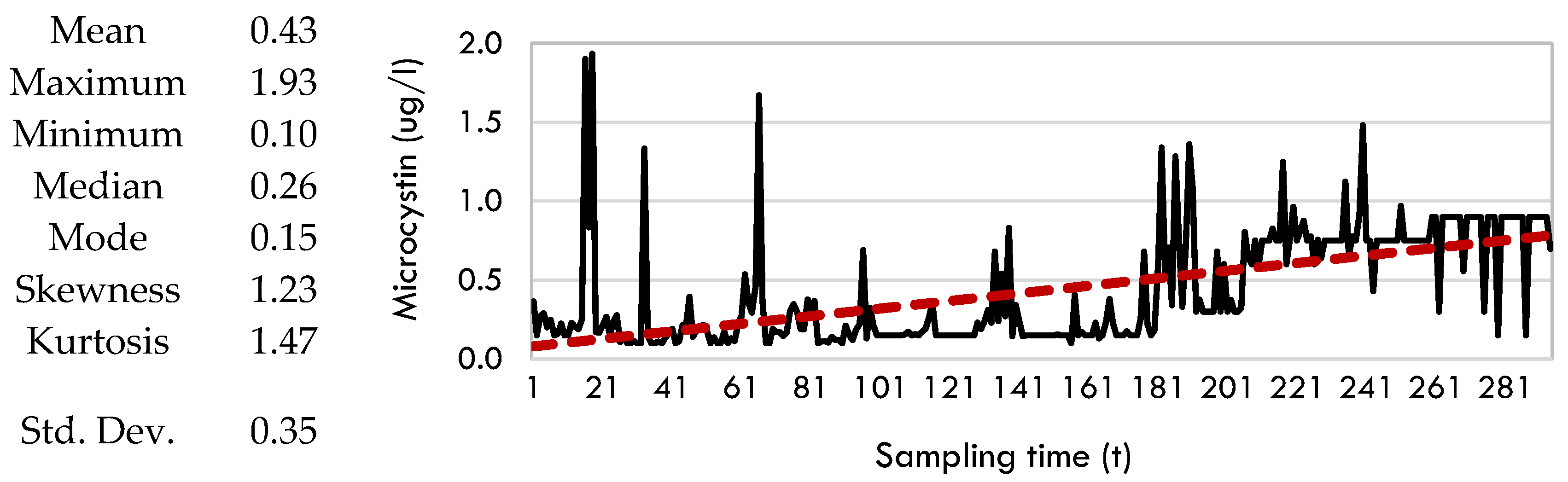
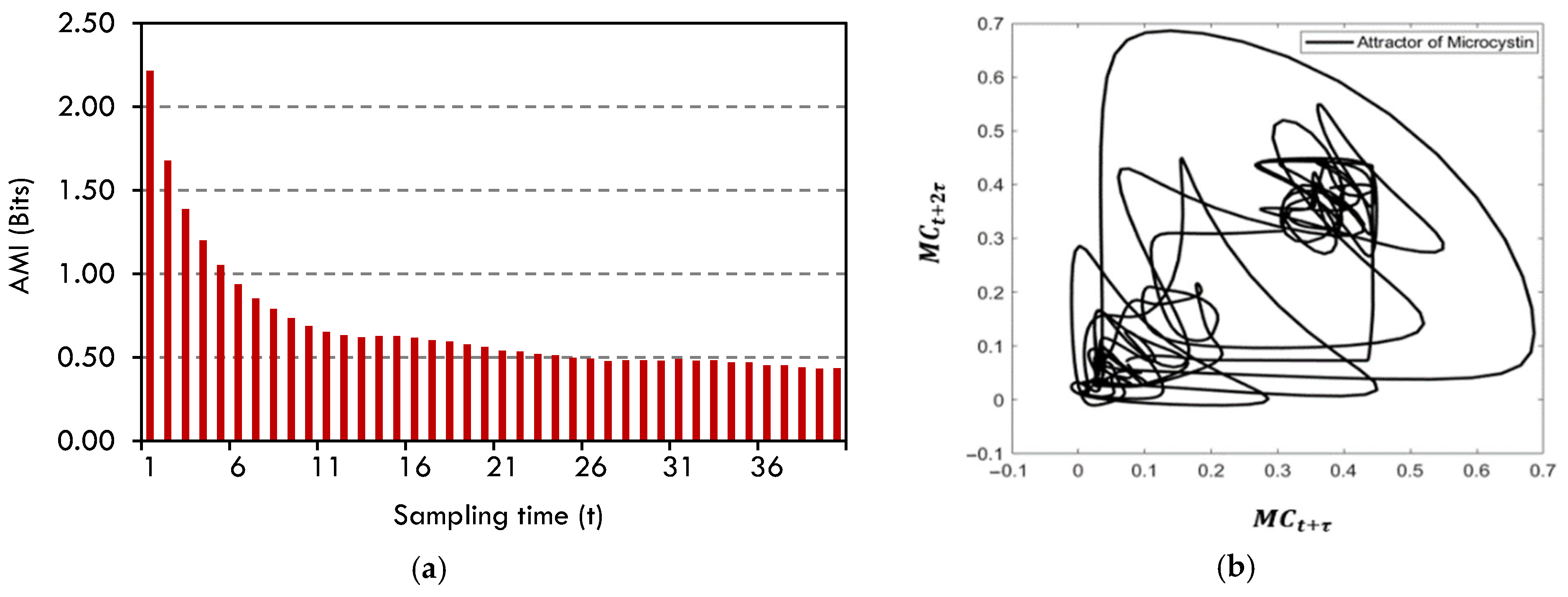
2. Results and Discussions
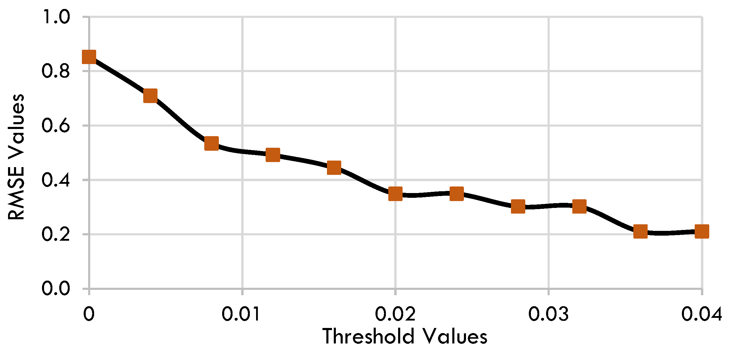
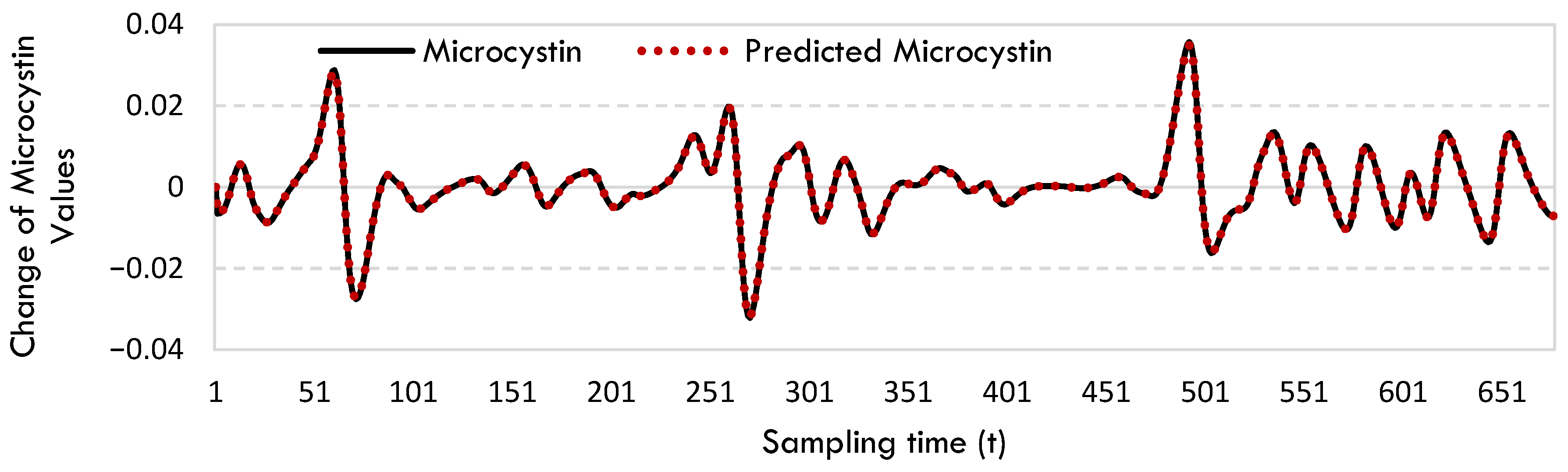
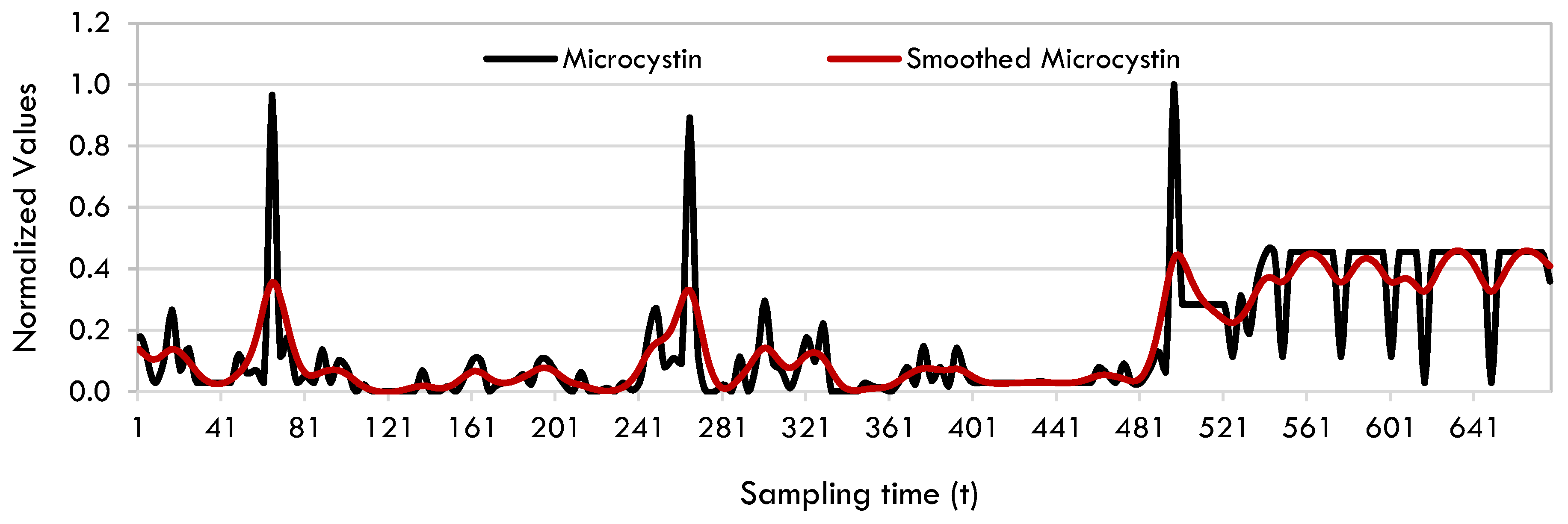
2.1. SINDy Model
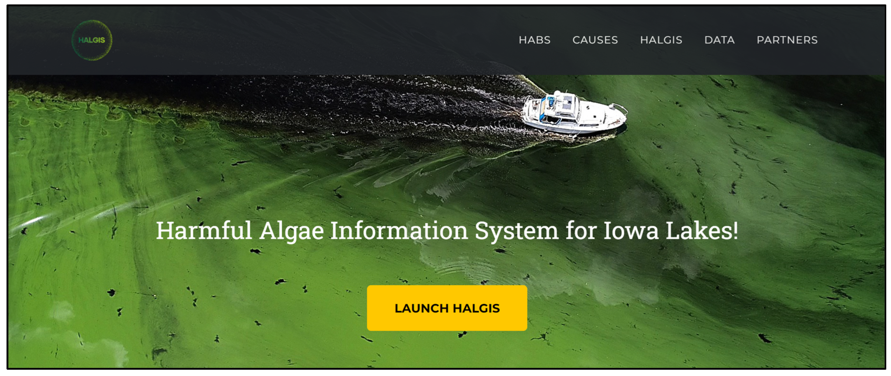
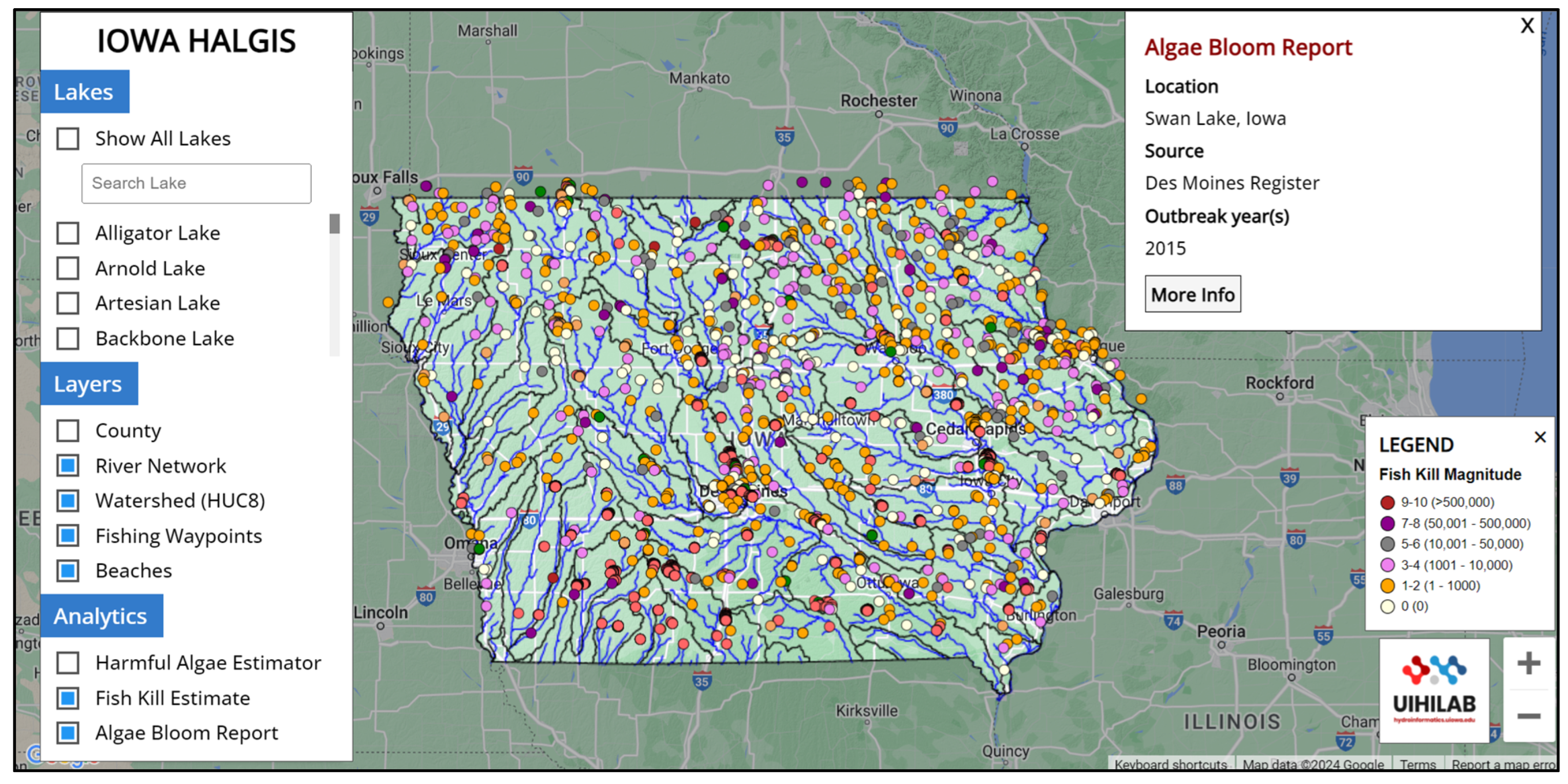
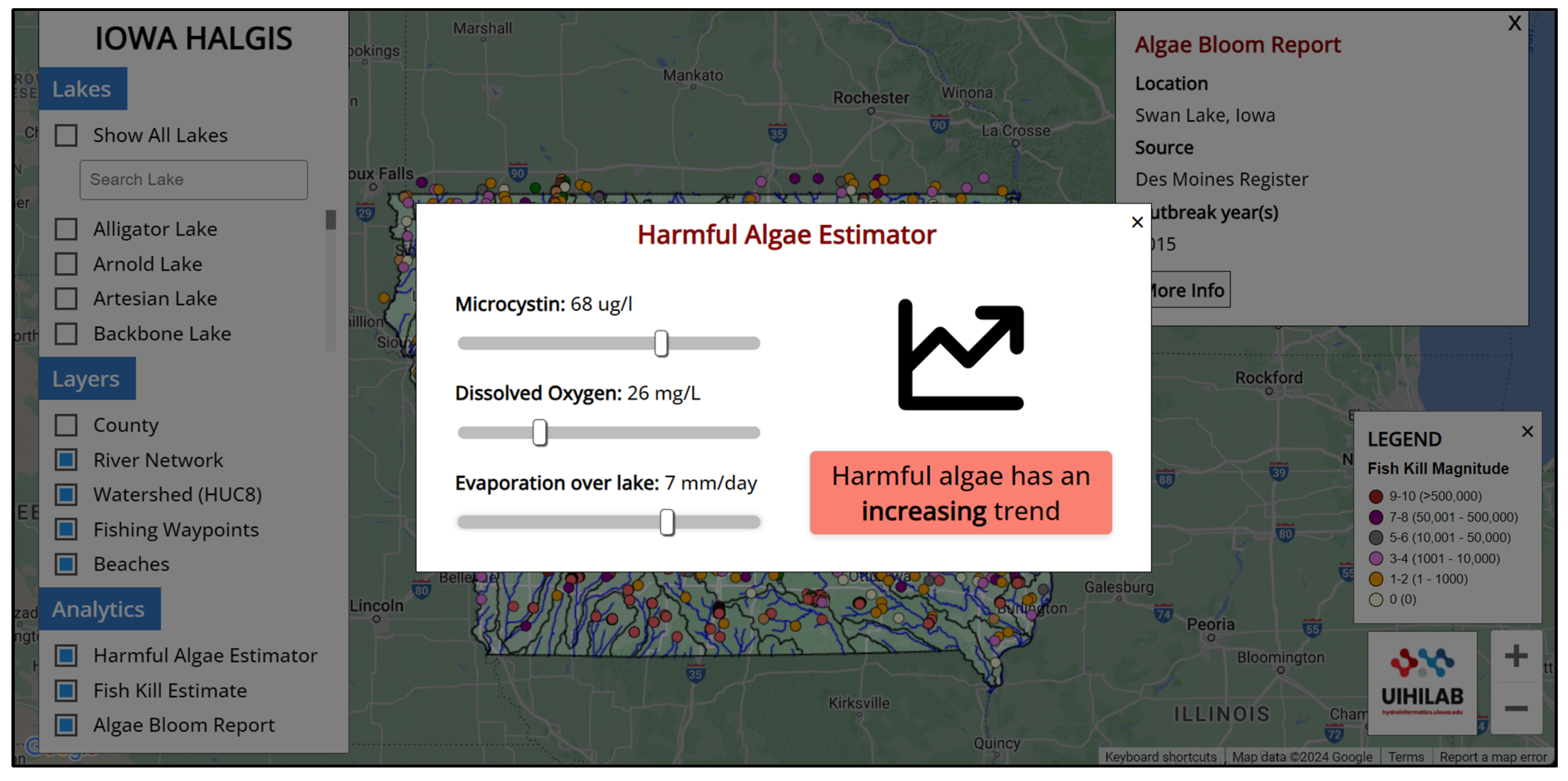
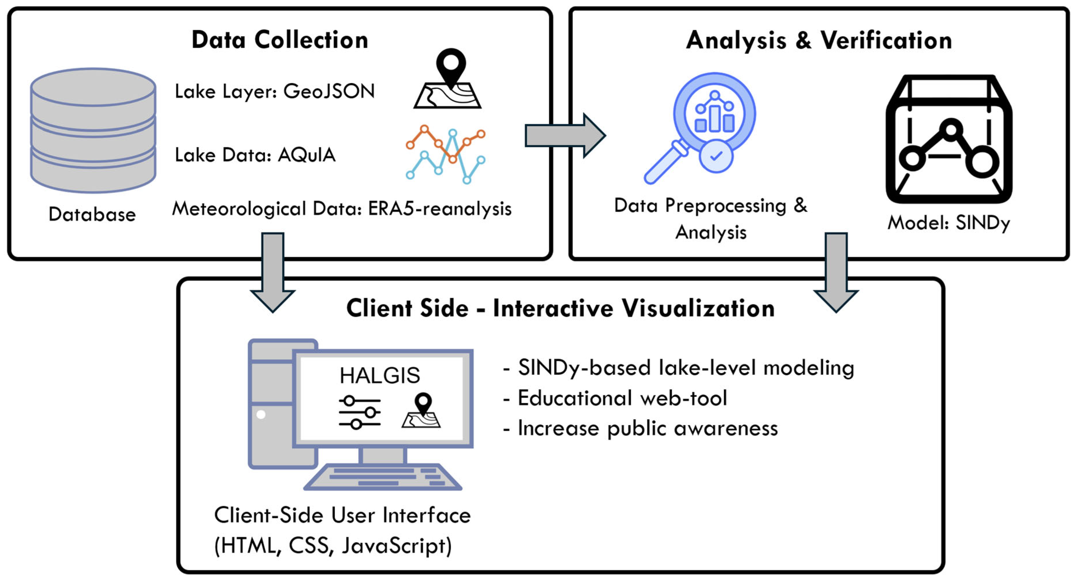
2.2. HALGIS Web Framework
3. Conclusions
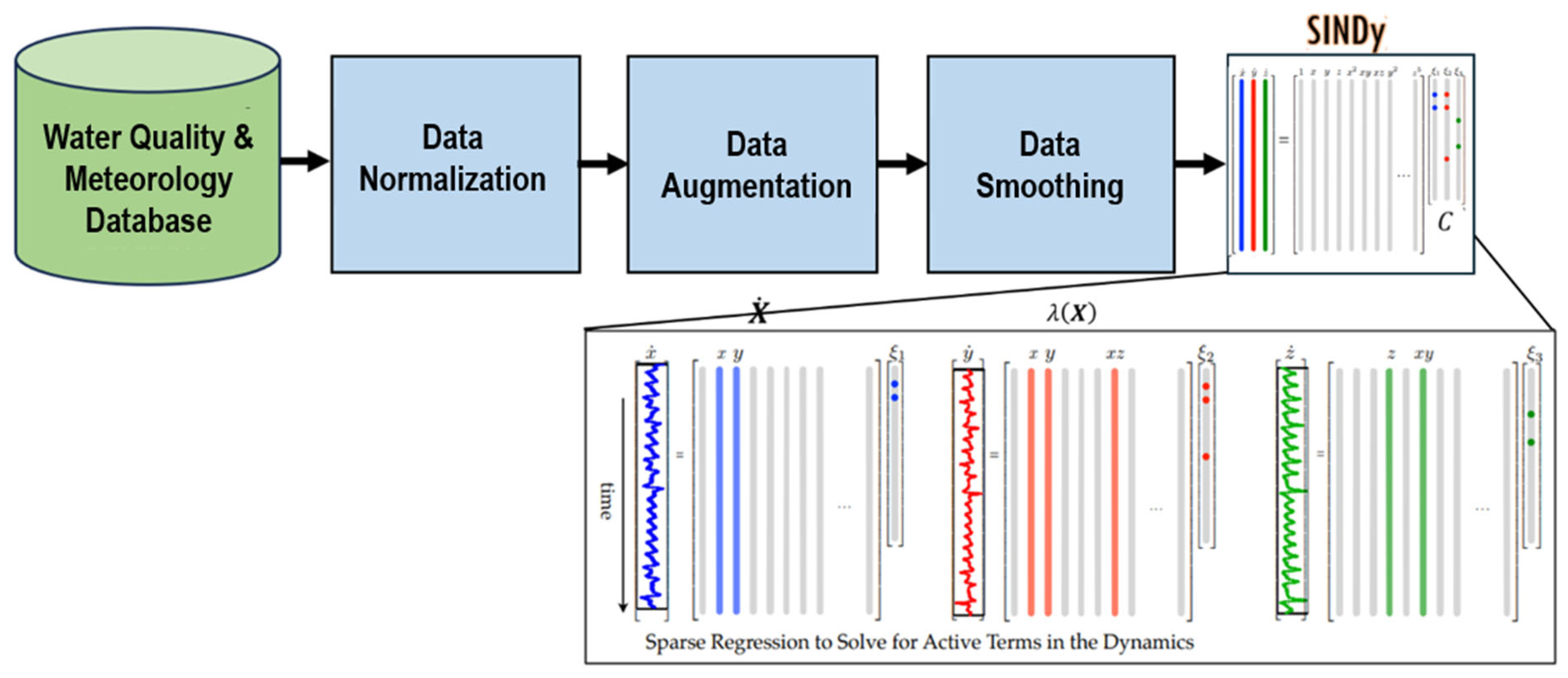
4. Materials and Methods
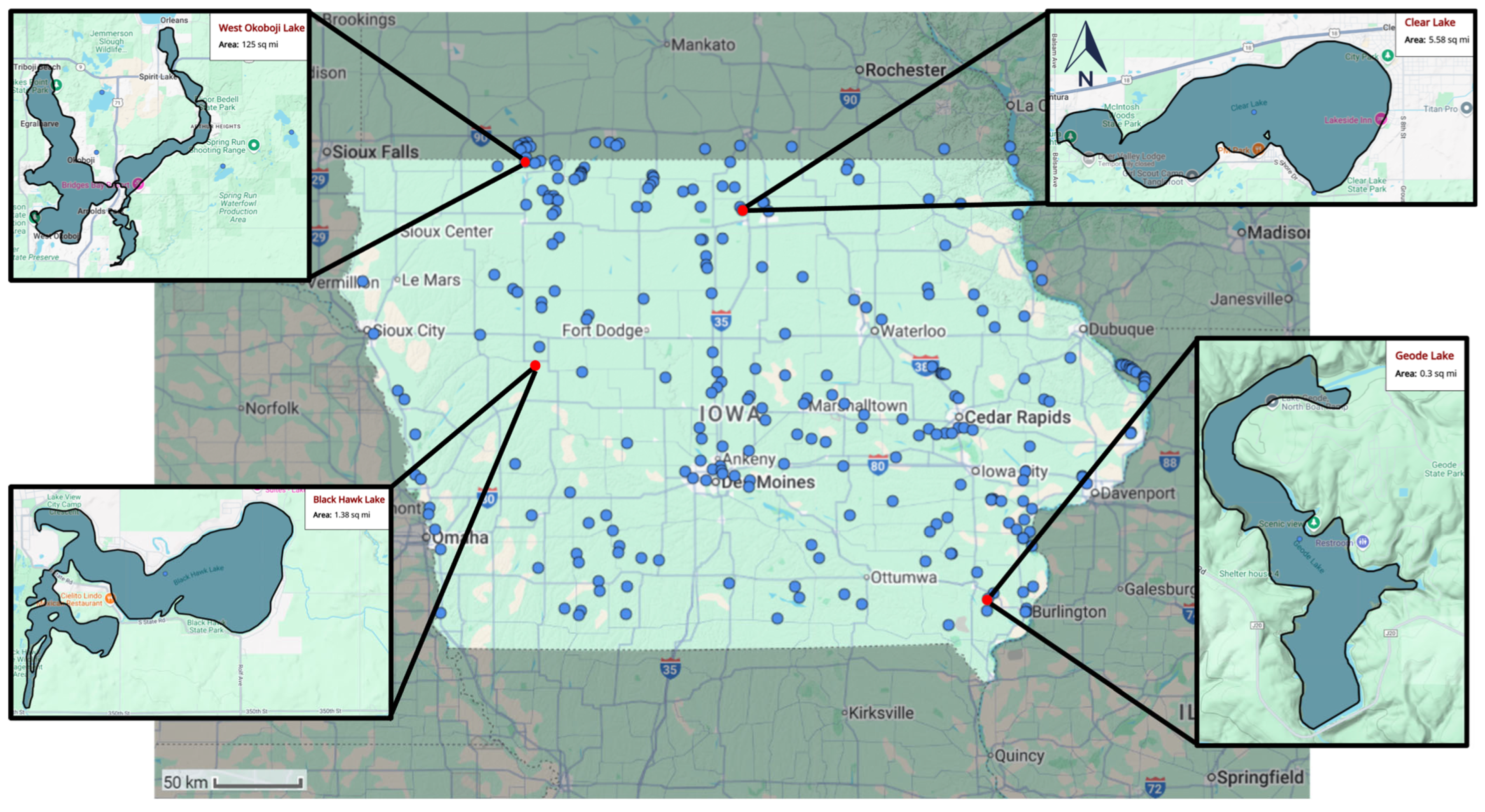
4.1. Study Area
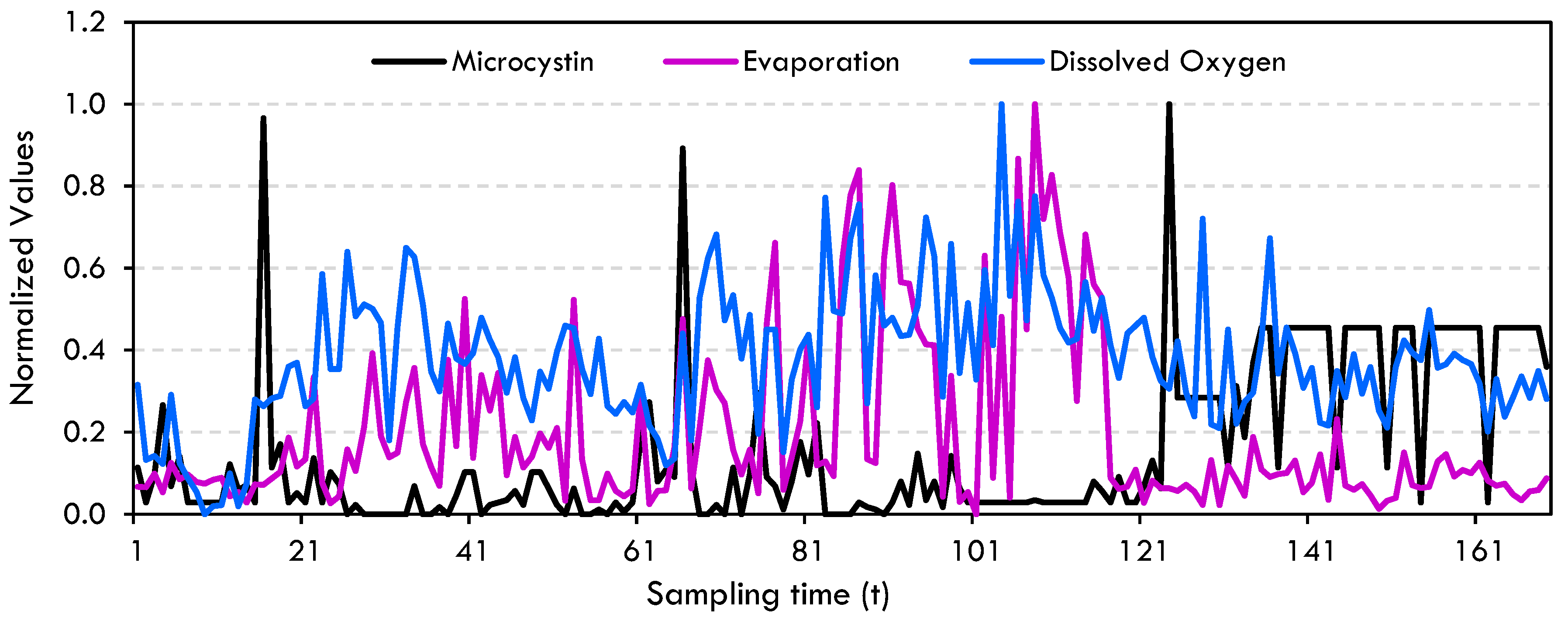
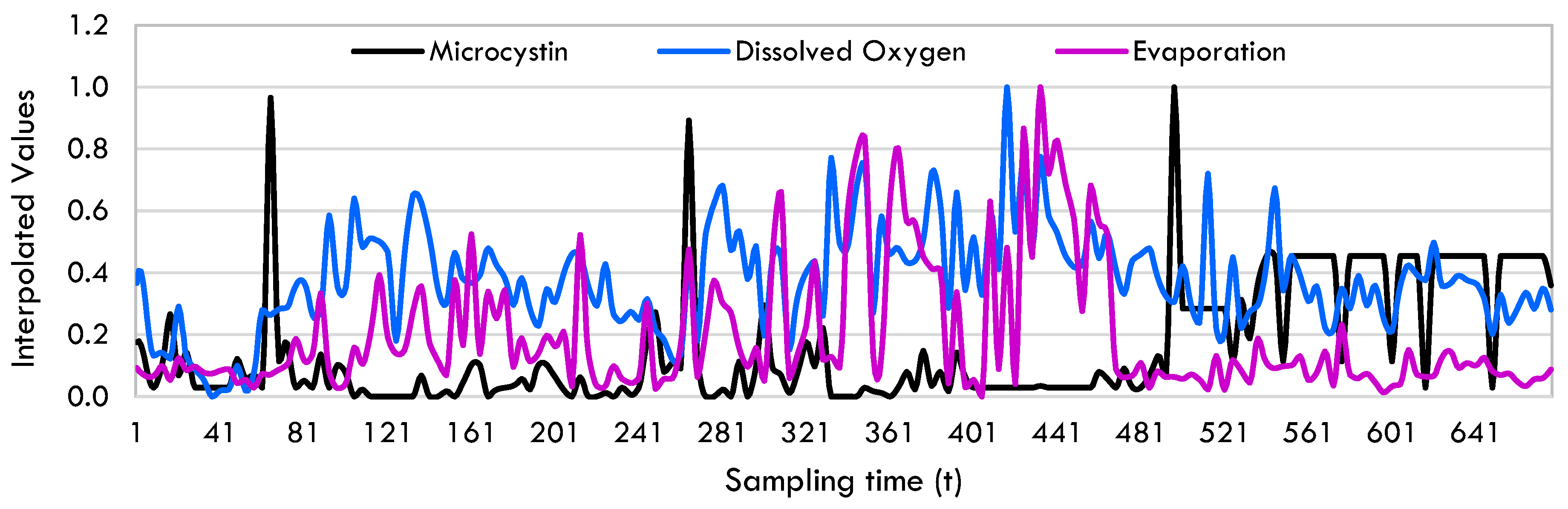
4.2. Case Study
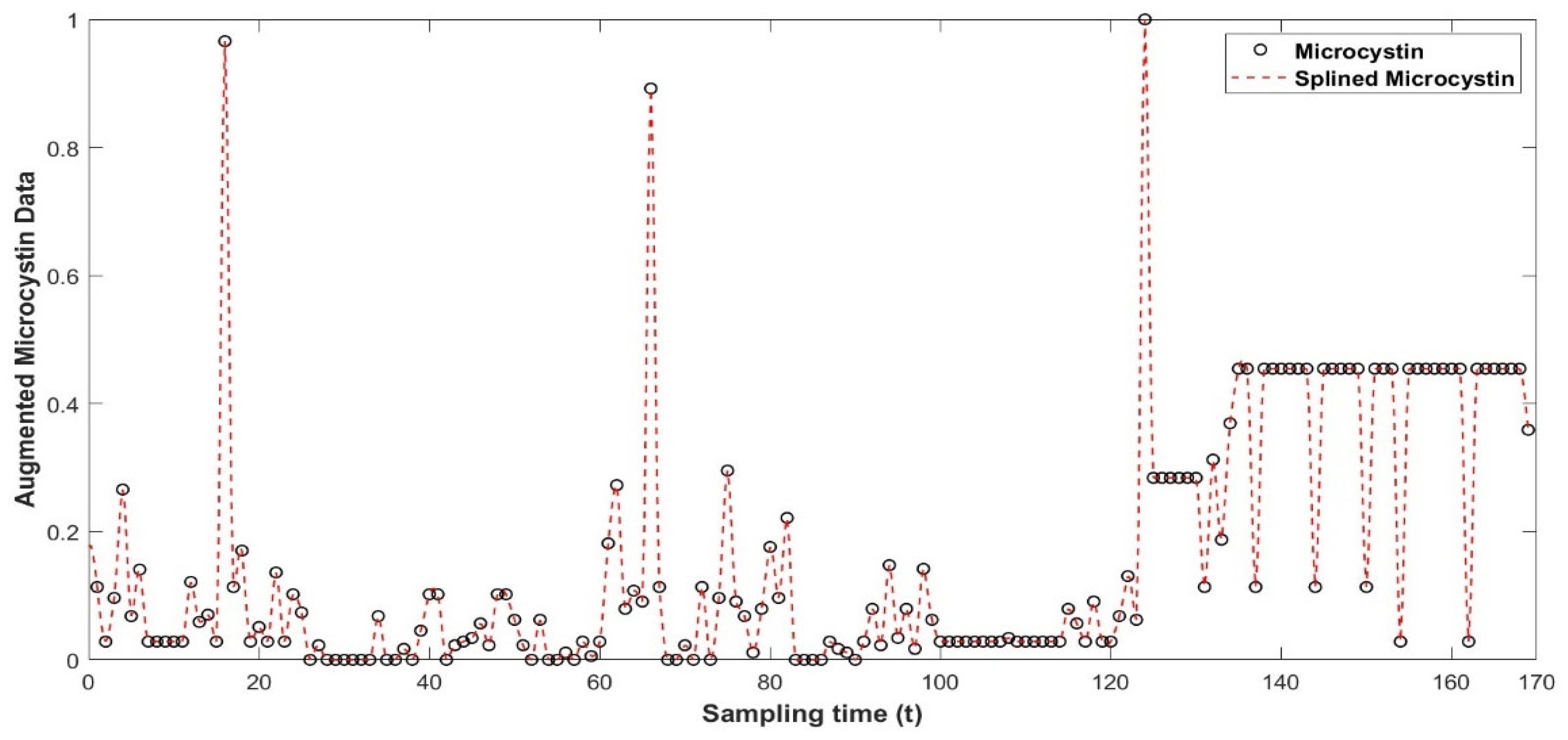
Data Preprocessing
4.3. Sparse Identification of Nonlinear Dynamics (SINDy)
4.4. HALGIS Web Framework
Author Contributions
Funding
Institutional Review Board Statement
Informed Consent Statement
Data Availability Statement
Acknowledgments
Conflicts of Interest
References
- Schindler, D.W. Recent advances in the understanding and management of eutrophication. Limnol. Oceanogr. 2006, 51, 356–363. [Google Scholar] [CrossRef]
- Paerl, H.W.; Gardner, W.S.; Havens, K.E.; Joyner, A.R.; McCarthy, M.J.; Newell, S.E.; Qin, B.; Scott, J.T. Mitigating cyanobacterial harmful algal blooms in aquatic ecosystems impacted by climate change and anthropogenic nutrients. Harmful Algae 2016, 54, 213–222. [Google Scholar] [CrossRef] [PubMed]
- Rolim, S.B.A.; Veettil, B.K.; Vieiro, A.P.; Kessler, A.B.; Gonzatti, C. Remote sensing for mapping algal blooms in freshwater lakes: A review. Environ. Sci. Pollut. Res. 2023, 30, 19602–19616. [Google Scholar] [CrossRef]
- Gobler, C.J. Climate change and harmful algal blooms: Insights and perspective. Harmful Algae 2020, 91, 101731. [Google Scholar] [CrossRef] [PubMed]
- Graham, J.L.; Dubrovsky, N.M.; Eberts, S.M. Cyanobacterial Harmful Algal Blooms and US Geological Survey Science Capabilities; US Department of the Interior: Washington, DC, USA; US Geological Survey: Reston, VA, USA, 2016. [Google Scholar] [CrossRef]
- Coffey, R.; Paul, M.J.; Stamp, J.; Hamilton, A.; Johnson, T. A review of water quality responses to air temperature and precipitation changes 2: Nutrients, algal blooms, sediment, pathogens. J. Am. Water Resour. Assoc. 2019, 55, 844–868. [Google Scholar] [CrossRef]
- Li, Q.; Li, Q.; Wu, J.; He, K.; Xia, Y.; Liu, J.; Wang, F.; Cheng, Y. Wellhead Stability During Development Process of Hydrate Reservoir in the Northern South China Sea: Sensitivity Analysis. Processes 2025, 13, 1630. [Google Scholar] [CrossRef]
- CDC. Harmful Algal Bloom (HAB) Associated Illness. 2021. Available online: https://www.cdc.gov/habs/general.html (accessed on 23 February 2023).
- Bakanoğulları, F.; Şaylan, L.; Yeşilköy, S. Effects of phenological stages, growth and meteorological factor on the albedo of different crop cultivars. Ital. J. Agrometeorol. 2022, 1, 23–40. [Google Scholar] [CrossRef]
- Yeşilköy, S.; Demir, I. Crop yield prediction based on reanalysis and crop phenology data in the agroclimatic zones. Theor. Appl. Climatol. 2024, 155, 7035–7048. [Google Scholar] [CrossRef]
- Ralston, D.K.; Moore, S.K. Modeling harmful algal blooms in a changing climate. Harmful Algae 2020, 91, 101729. [Google Scholar] [CrossRef]
- Paerl, H.W.; Huisman, J. Blooms like it hot. Science 2008, 320, 57–58. [Google Scholar] [CrossRef]
- Paerl, H.W.; Paul, V.J. Climate change: Links to global expansion of harmful cyanobacteria. Water Res. 2012, 46, 1349–1363. [Google Scholar] [CrossRef] [PubMed]
- Lad, A.; Breidenbach, J.D.; Su, R.C.; Murray, J.; Kuang, R.; Mascarenhas, A.; Najjar, J.; Patel, S.; Hegde, P.; Youssef, M.; et al. As we drink and breathe: Adverse health effects of microcystins and other harmful algal bloom toxins in the liver, gut, lungs and beyond. Life 2022, 12, 418. [Google Scholar] [CrossRef] [PubMed]
- Li, B.; Zhang, X.; Wu, G.; Qin, B.; Tefsen, B.; Wells, M. Toxins from harmful algal blooms: How copper and iron render chalkophore a predictor of microcystin production. Water Res. 2023, 244, 120490. [Google Scholar] [CrossRef] [PubMed]
- Brookfield, A.E.; Hansen, A.T.; Sullivan, P.L.; Czuba, J.A.; Kirk, M.F.; Li, L.; Newcomer, M.E.; Wilkinson, G. Predicting algal blooms: Are we overlooking groundwater? Sci. Total Environ. 2021, 769, 144442. [Google Scholar] [CrossRef]
- Ruiz-Villarreal, M.; García-García, L.M.; Cobas, M.; Díaz, P.A.; Reguera, B. Modelling the hydrodynamic conditions associated with Dinophysis blooms in Galicia (NW Spain). Harmful Algae 2016, 53, 40–52. [Google Scholar] [CrossRef]
- Díaz, P.A.; Ruiz-Villarreal, M.; Pazos, Y.; Moita, T.; Reguera, B. Climate variability and Dinophysis acuta blooms in an upwelling system. Harmful Algae 2016, 53, 145–159. [Google Scholar] [CrossRef]
- Moe, S.J.; Haande, S.; Couture, R.M. Climate change, cyanobacteria blooms and ecological status of lakes: A Bayesian network approach. Ecol. Model. 2016, 337, 330–347. [Google Scholar] [CrossRef]
- Baydaroğlu, Ö.; Koçak, K. Spatiotemporal analysis of wind speed via the Bayesian maximum entropy approach. Environ. Earth Sci. 2019, 78, 17. [Google Scholar] [CrossRef]
- Baydaroğlu, Ö. Harmful algal bloom prediction using empirical dynamic modeling. Sci. Total Environ. 2025, 959, 178185. [Google Scholar] [CrossRef]
- Ye, H.; Beamish, R.J.; Glaser, S.M.; Grant, S.C.; Hsieh, C.H.; Richards, L.J.; Schnute, J.T.; Sugihara, G. Equation-free mechanistic ecosystem forecasting using empirical dynamic modeling. Proc. Natl. Acad. Sci. USA 2015, 112, E1569–E1576. [Google Scholar] [CrossRef]
- Anderson, C.R.; Moore, S.K.; Tomlinson, M.C.; Silke, J.; Cusack, C.K. Living with harmful algal blooms in a changing world: Strategies for modeling and mitigating their effects in coastal marine ecosystems. In Coastal and Marine Hazards, Risks, and Disasters; Elsevier: Amsterdam, The Netherlands, 2015; pp. 495–561. [Google Scholar] [CrossRef]
- Hallegraeff, G.M. Ocean climate change, phytoplankton community responses, and harmful algal blooms: A formidable predictive challenge 1. J. Phycol. 2010, 46, 220–235. [Google Scholar] [CrossRef]
- Treuer, G.; Kirchhoff, C.; Lemos, M.C.; McGrath, F. Challenges of managing harmful algal blooms in US drinking water systems. Nat. Sustain. 2021, 4, 958–964. [Google Scholar] [CrossRef]
- Zhang, Y.; Shi, K.; Liu, J.; Deng, J.; Qin, B.; Zhu, G.; Zhou, Y. Meteorological and hydrological conditions driving the formation and disappearance of black blooms, an ecological disaster phenomena of eutrophication and algal blooms. Sci. Total Environ. 2016, 569, 1517–1529. [Google Scholar] [CrossRef]
- Maniyar, C.B.; Kumar, A.; Mishra, D.R. Continuous and synoptic assessment of Indian inland waters for harmful algae blooms. Harmful Algae 2022, 111, 102160. [Google Scholar] [CrossRef]
- Townhill, B.L.; Tinker, J.; Jones, M.; Pitois, S.; Creach, V.; Simpson, S.D.; Dye, S.; Bear, E.; Pinnegar, J.K. Harmful algal blooms and climate change: Exploring future distribution changes. ICES J. Mar. Sci. 2018, 76, 353. [Google Scholar] [CrossRef]
- Trainer, V.L.; Moore, S.K.; Hallegraeff, G.; Kudela, R.M.; Clement, A.; Mardones, J.I.; Cochlan, W.P. Pelagic harmful algal blooms and climate change: Lessons from nature’s experiments with extremes. Harmful Algae 2020, 91, 101591. [Google Scholar] [CrossRef]
- Gobler, C.J.; Doherty, O.M.; Hattenrath-Lehmann, T.K.; Griffith, A.W.; Kang, Y.; Litaker, R.W. Ocean warming since 1982 has expanded the niche of toxic algal blooms in the North Atlantic and North Pacific oceans. Proc. Natl. Acad. Sci. USA 2017, 114, 4975–4980. [Google Scholar] [CrossRef]
- Hou, X.; Feng, L.; Dai, Y.; Hu, C.; Gibson, L.; Tang, J.; Lee, Z.; Wang, Y.; Cai, X.; Liu, J.; et al. Global mapping reveals increase in lacustrine algal blooms over the past decade. Nat. Geosci. 2022, 15, 130–134. [Google Scholar] [CrossRef]
- Ho, J.C.; Michalak, A.M. Exploring temperature and precipitation impacts on harmful algal blooms across continental US lakes. Limnol. Oceanogr. 2020, 65, 992–1009. [Google Scholar] [CrossRef]
- Zhou, Y.; Yan, W.; Wei, W. Effect of sea surface temperature and precipitation on annual frequency of harmful algal blooms in the East China Sea over the past decades. Environ. Pollut. 2021, 270, 116224. [Google Scholar] [CrossRef]
- Deng, J.; Chen, F.; Liu, X.; Peng, J.; Hu, W. Horizontal migration of algal patches associated with cyanobacterial blooms in an eutrophic shallow lake. Ecol. Eng. 2016, 87, 185–193. [Google Scholar] [CrossRef]
- Hamilton, D.S.; Perron, M.M.; Bond, T.C.; Bowie, A.R.; Buchholz, R.R.; Guieu, C.; Ito, A.; Maenhaut, W.; Myriokefalitakis, S.; Olgun, N.; et al. Earth, wind, fire, and pollution: Aerosol nutrient sources and impacts on ocean biogeochemistry. Annu. Rev. Mar. Sci. 2022, 14, 303–330. [Google Scholar] [CrossRef] [PubMed]
- Liu, S.T.; Zhang, L. Surface Chaotic Theory and the Growth of Harmful Algal Bloom. In Surface Chaos and Its Applications; Springer Nature: Singapore, 2022; pp. 299–320. [Google Scholar] [CrossRef]
- Huo, S.; He, Z.; Ma, C.; Zhang, H.; Xi, B.; Xia, X.; Xu, Y.; Wu, F. Stricter nutrient criteria are required to mitigate the impact of climate change on harmful cyanobacterial blooms. J. Hydrol. 2019, 569, 698–704. [Google Scholar] [CrossRef]
- Michalak, A.M.; Anderson, E.J.; Beletsky, D.; Boland, S.; Bosch, N.S.; Bridgeman, T.B.; Chaffin, J.D.; Cho, K.; Confesor, R.; Daloğlu, I.; et al. Record-setting algal bloom in Lake Erie caused by agricultural and meteorological trends consistent with expected future conditions. Proc. Natl. Acad. Sci. USA 2013, 110, 6448–6452. [Google Scholar] [CrossRef]
- Islam, S.S.; Yeşilköy, S.; Baydaroğlu, Ö.; Yıldırım, E.; Demir, I. State-level multidimensional agricultural drought susceptibility and risk assessment for agriculturally prominent areas. Int. J. River Basin Manag. 2024, 23, 337–354. [Google Scholar] [CrossRef]
- Wilkinson, G.M.; Walter, J.A.; Albright, E.A.; King, R.F.; Moody, E.K.; Ortiz, D.A. An evaluation of statistical models of microcystin detection in lakes applied forward under varying climate conditions. Harmful Algae 2024, 137, 102679. [Google Scholar] [CrossRef]
- Greene, S.B.D.; LeFevre, G.H.; Markfort, C.D. Improving the spatial and temporal monitoring of cyanotoxins in Iowa lakes using a multiscale and multi-modal monitoring approach. Sci. Total Environ. 2021, 760, 143327. [Google Scholar] [CrossRef]
- Lee, J.; Choi, J.; Fatka, M.; Swanner, E.; Ikuma, K.; Liang, X.; Leung, T.; Howe, A. Improved detection of mcyA genes and their phylogenetic origins in harmful algal blooms. Water Res. 2020, 176, 115730. [Google Scholar] [CrossRef]
- Villanueva, P.; Yang, J.; Radmer, L.; Liang, X.; Leung, T.; Ikuma, K.; Swanner, E.D.; Howe, A.; Lee, J. One-Week-Ahead Prediction of Cyanobacterial Harmful Algal Blooms in Iowa Lakes. Environ. Sci. Technol. 2023, 57, 20636–20646. [Google Scholar] [CrossRef]
- Kim, J.; Jones, J.R.; Seo, D. Factors affecting harmful algal bloom occurrence in a river with regulated hydrology. J. Hydrol. Reg. Stud. 2021, 33, 100769. [Google Scholar] [CrossRef]
- Wang, C.; Wang, Z.; Wang, P.; Zhang, S. Multiple effects of environmental factors on algal growth and nutrient thresholds for harmful algal blooms: Application of response surface methodology. Environ. Model. Assess. 2016, 21, 247–259. [Google Scholar] [CrossRef]
- Yu, X.; Yuan, S.; Zhang, T. The effects of toxin-producing phytoplankton and environmental fluctuations on the planktonic blooms. Nonlinear Dyn. 2018, 91, 1653–1668. [Google Scholar] [CrossRef]
- Hallegraeff, G.M.; Anderson, D.M.; Belin, C.; Bottein, M.Y.D.; Bresnan, E.; Chinain, M.; Enevoldsen, H.; Iwataki, M.; Karlson, B.; McKenzie, C.H.; et al. Perceived global increase in algal blooms is attributable to intensified monitoring and emerging bloom impacts. Commun. Earth Environ. 2021, 2, 117. [Google Scholar] [CrossRef]
- Lee, J.; Jeon, W.; Chang, M.; Han, M.S. Evaluation of rapid cell division in non-uniform cell cycles. J. Basic Microbiol. 2015, 55, 1159–1167. [Google Scholar] [CrossRef]
- Guo, J.; Dong, Y.; Lee, J.H. A real time data driven algal bloom risk forecast system for mariculture management. Mar. Pollut. Bull. 2020, 161, 111731. [Google Scholar] [CrossRef]
- Wang, X.; Bouzembrak, Y.; Marvin, H.J.; Clarke, D.; Butler, F. Bayesian Networks modeling of diarrhetic shellfish poisoning in Mytilus edulis harvested in Bantry Bay, Ireland. Harmful Algae 2022, 112, 102171. [Google Scholar] [CrossRef]
- Janssen, A.B.; Janse, J.H.; Beusen, A.H.; Chang, M.; Harrison, J.A.; Huttunen, I.; Kong, X.; Rost, J.; Teurlincx, S.; Troost, T.A.; et al. How to model algal blooms in any lake on earth. Curr. Opin. Environ. Sustain. 2019, 36, 1–10. [Google Scholar] [CrossRef]
- Brunton, S.L.; Proctor, J.L.; Kutz, J.N. Discovering governing equations from data by sparse identification of nonlinear dynamical systems. Proc. Natl. Acad. Sci. USA 2016, 113, 3932–3937. [Google Scholar] [CrossRef]
- Zhang, D.; Savage, T.R.; Cho, B.A. Combining model structure identification and hybrid modelling for photo-production process predictive simulation and optimisation. Biotechnol. Bioeng. 2020, 117, 3356–3367. [Google Scholar] [CrossRef]
- Corbetta, M. Application of sparse identification of nonlinear dynamics for physics-informed learning. In Proceedings of the 2020 IEEE Aerospace Conference, Big Sky, MT, USA, 7–14 March 2020; IEEE: Piscataway, NJ, USA, 2020; pp. 1–8. [Google Scholar] [CrossRef]
- Joedicke, D.; Parra, D.; Kronberger, G.; Winkler, S.M. Identifying differential equations for the prediction of blood glucose using sparse identification of nonlinear systems. In Proceedings of the International Conference on Computer Aided Systems Theory, Las Palmas de Gran Canaria, Spain, 20–25 February 2022; Springer Nature: Cham, Switzerland, 2022; pp. 181–188. [Google Scholar] [CrossRef]
- Rubio-Herrero, J.; Marrero, C.O.; Fan, W.T.L. Modeling atmospheric data and identifying dynamics Temporal data-driven modeling of air pollutants. J. Clean. Prod. 2022, 333, 129863. [Google Scholar] [CrossRef]
- Kaiser, E.; Kutz, J.N.; Brunton, S.L. Sparse identification of nonlinear dynamics for model predictive control in the low-data limit. Proc. R. Soc. A 2018, 474, 20180335. [Google Scholar] [CrossRef] [PubMed]
- Yeşilköy, S.; Baydaroglu, O.; Singh, N.; Sermet, Y.; Demir, I. A contemporary systematic review of Cyberinfrastructure Systems and Applications for Flood and Drought Data Analytics and Communication. Environ. Res. Commun. 2024, 6, 102003. [Google Scholar] [CrossRef]
- Albano, R.; Sole, A.; Adamowski, J. READY: A web-based geographical information system for enhanced flood resilience through raising awareness in citizens. Nat. Hazards Earth Syst. Sci. 2015, 15, 1645–1658. [Google Scholar] [CrossRef]
- Iyengar, S.; Massey, D.S. Scientific communication in a post-truth society. Proc. Natl. Acad. Sci. USA 2019, 116, 7656–7661. [Google Scholar] [CrossRef]
- Shr, Y.H.; Zhang, W. Do Iowa Residents and Farmers Care about Improving Water Quality and Reducing Harmful Algal Blooms?: Results from Two Household Surveys. Center for Agricultural and Rural Development. 2021. Available online: https://www.card.iastate.edu/products/publications/pdf/21pb32.pdf (accessed on 2 July 2025).
- Champion, K.; Zheng, P.; Aravkin, A.Y.; Brunton, S.L.; Kutz, J.N. A unified sparse optimization framework to learn parsimonious physics-informed models from data. IEEE Access 2020, 8, 169259–169271. [Google Scholar] [CrossRef]
- Champion, K.P.; Brunton, S.L.; Kutz, J.N. Discovery of nonlinear multiscale systems: Sampling strategies and embeddings. SIAM J. Appl. Dyn. Syst. 2019, 18, 312–333. [Google Scholar] [CrossRef]
- França, T.; Braga, A.M.B.; Ayala, H.V.H. Feature engineering to cope with noisy data in sparse identification. Expert Syst. Appl. 2022, 188, 115995. [Google Scholar] [CrossRef]
- Lisci, S.; Gitani, E.; Mulas, M.; Tronci, S. Modeling a Biological Reactor using Sparse Identification Method. Chem. Eng. Trans. 2021, 86, 901–906. [Google Scholar] [CrossRef]
- Moazeni, F.; Khazaei, J. Data-enabled identification of nonlinear dynamics of water systems using sparse regression technique. IFAC-PapersOnLine 2023, 56, 2389–2394. [Google Scholar] [CrossRef]
- Takens, F. Detecting strange attractors in turbulence. In Dynamical Systems and Turbulence, Warwick 1980: Proceedings of a Symposium Held at the University of Warwick 1979/80; Springer: Berlin/Heidelberg, Germany, 2006; pp. 366–381. [Google Scholar]
- Fraser, A.M.; Swinney, H.L. Independent coordinates for strange attractors from mutual information. Phys. Rev. A 1986, 33, 1134. [Google Scholar] [CrossRef]
- Grassberger, P.; Schreiber, T.; Schaffrath, C. Nonlinear time sequence analysis. Int. J. Bifurc. Chaos 1991, 1, 521–547. [Google Scholar] [CrossRef]
- Kantz, H. A robust method to estimate the maximal Lyapunov exponent of a time series. Phys. Lett. A 1994, 185, 77–87. [Google Scholar] [CrossRef]
- de Silva, B.M.; Champion, K.; Quade, M.; Loiseau, J.C.; Kutz, J.N.; Brunton, S.L. Pysindy: A python package for the sparse identification of nonlinear dynamics from data. arXiv 2020. [Google Scholar] [CrossRef]
- Kaptanoglu, A.A.; de Silva, B.M.; Fasel, U.; Kaheman, K.; Goldschmidt, A.J.; Callaham, J.L.; Delahunt, C.B.; Nicolaou, Z.G.; Champion, K.; Loiseau, J.-C.; et al. PySINDy: A comprehensive Python package for robust sparse system identification. arXiv 2021. [Google Scholar] [CrossRef]
- Abdullah, F.; Alhajeri, M.S.; Christofides, P.D. Modeling and control of nonlinear processes using sparse identification: Using dropout to handle noisy data. Ind. Eng. Chem. Res. 2022, 61, 17976–17992. [Google Scholar] [CrossRef]
- Fukami, K.; Murata, T.; Zhang, K.; Fukagata, K. Sparse identification of nonlinear dynamics with low-dimensionalized flow representations. J. Fluid Mech. 2021, 926, A10. [Google Scholar] [CrossRef]
- Akima, H. A new method of interpolation and smooth curve fitting based on local procedures. J. ACM 1970, 17, 589–602. [Google Scholar] [CrossRef]
- Mohamad, N.B.; Lai, A.C.; Lim, B.H. A case study in the tropical region to evaluate univariate imputation methods for solar irradiance data with different weather types. Sustain. Energy Technol. Assess. 2022, 50, 101764. [Google Scholar] [CrossRef]
- Baydaroğlu, Ö.; Demir, I. Temporal and spatial satellite data augmentation for deep learning-based rainfall nowcasting. J. Hydroinform. 2024, 26, 589–607. [Google Scholar] [CrossRef]
- Baydaroğlu, Ö.; Muste, M.; Cikmaz, A.B.; Kim, K.; Meselhe, E.; Demir, I. Testing protocols for smoothing datasets of hydraulic variables acquired during unsteady flows. Hydrol. Sci. J. 2024, 69, 1813–1830. [Google Scholar] [CrossRef]
- Cortiella, A.; Park, K.C.; Doostan, A. A priori denoising strategies for sparse identification of nonlinear dynamical systems: A comparative study. J. Comput. Inf. Sci. Eng. 2023, 23, 011004. [Google Scholar] [CrossRef]
- Henderson, R. A new method of graduation. Trans. Actuar. Soc. Am. 1924, 25, 29–40. [Google Scholar]
- Henderson, R. Further remarks on graduation. Trans. Actuar. Soc. Am. 1925, 26, 52–57. [Google Scholar]
- Whittaker, E.T. On a new method of graduation. Proc. Edinb. Math. Soc. 1922, 41, 63–75. [Google Scholar] [CrossRef]
- Whittaker, E.T. VIII.—On the Theory of Graduation. Proc. R. Soc. Edinb. 1925, 44, 77–83. [Google Scholar] [CrossRef]
- Yuan, Z. Applications of Sparse Identification of Nonlinear Dynamical Systems. Ph.D. Dissertation, California State Polytechnic University, Pomona, CA, USA, 2023. [Google Scholar]
- Kadah, N.; Özbek, N.S. Model Investigation of Nonlinear Dynamical Systems by Sparse Identification. Avrupa Bilim Teknol. Derg. 2020, 254–263. [Google Scholar] [CrossRef]


| Lake | r | RMSE | MAPE |
|---|---|---|---|
| West Okoboji | 0.99 | 0.0001 | 1.61 |
| McIntosh Woods | 0.69 | 0.0046 | 11.3 |
| Blackhawk | 0.99 | 0.0001 | 1.72 |
| Geode | 0.99 | 0.0047 | 1.95 |
| Site ID | Site Name |
|---|---|
| 21300001 | Gull Point Beach |
| 21300002 | Pikes Point Beach |
| 21300003 | Triboji Beach |
| 22300009 | West Okoboji Lake |
| 14000189 | Emerson Bay 1 |
| 14000190 | Emerson Bay 2 |
| 14000191 | Emerson Bay 3 |
| 14000193 | Emmerson T-4 |
| 14000410 | West Lake Okoboji-Smiths Bay |
| 14000411 | West Lake Okoboji-Millers Bay |
| 14000412 | West Lake Okoboji-Main Basin North |
| 15300001 | Unnamed tributary to Emerson Bay at beach |
Disclaimer/Publisher’s Note: The statements, opinions and data contained in all publications are solely those of the individual author(s) and contributor(s) and not of MDPI and/or the editor(s). MDPI and/or the editor(s) disclaim responsibility for any injury to people or property resulting from any ideas, methods, instructions or products referred to in the content. |
© 2025 by the authors. Licensee MDPI, Basel, Switzerland. This article is an open access article distributed under the terms and conditions of the Creative Commons Attribution (CC BY) license (https://creativecommons.org/licenses/by/4.0/).
Share and Cite
Baydaroğlu, Ö.; Yeşilköy, S.; Dave, A.; Linderman, M.; Demir, I. Modeling Algal Toxin Dynamics and Integrated Web Framework for Lakes. Toxins 2025, 17, 338. https://doi.org/10.3390/toxins17070338
Baydaroğlu Ö, Yeşilköy S, Dave A, Linderman M, Demir I. Modeling Algal Toxin Dynamics and Integrated Web Framework for Lakes. Toxins. 2025; 17(7):338. https://doi.org/10.3390/toxins17070338
Chicago/Turabian StyleBaydaroğlu, Özlem, Serhan Yeşilköy, Anchit Dave, Marc Linderman, and Ibrahim Demir. 2025. "Modeling Algal Toxin Dynamics and Integrated Web Framework for Lakes" Toxins 17, no. 7: 338. https://doi.org/10.3390/toxins17070338
APA StyleBaydaroğlu, Ö., Yeşilköy, S., Dave, A., Linderman, M., & Demir, I. (2025). Modeling Algal Toxin Dynamics and Integrated Web Framework for Lakes. Toxins, 17(7), 338. https://doi.org/10.3390/toxins17070338