A Feasibility Study of Sea Ice Motion and Deformation Measurements Using Multi-Sensor High-Resolution Optical Satellite Images


Abstract
1. Introduction
2. Materials
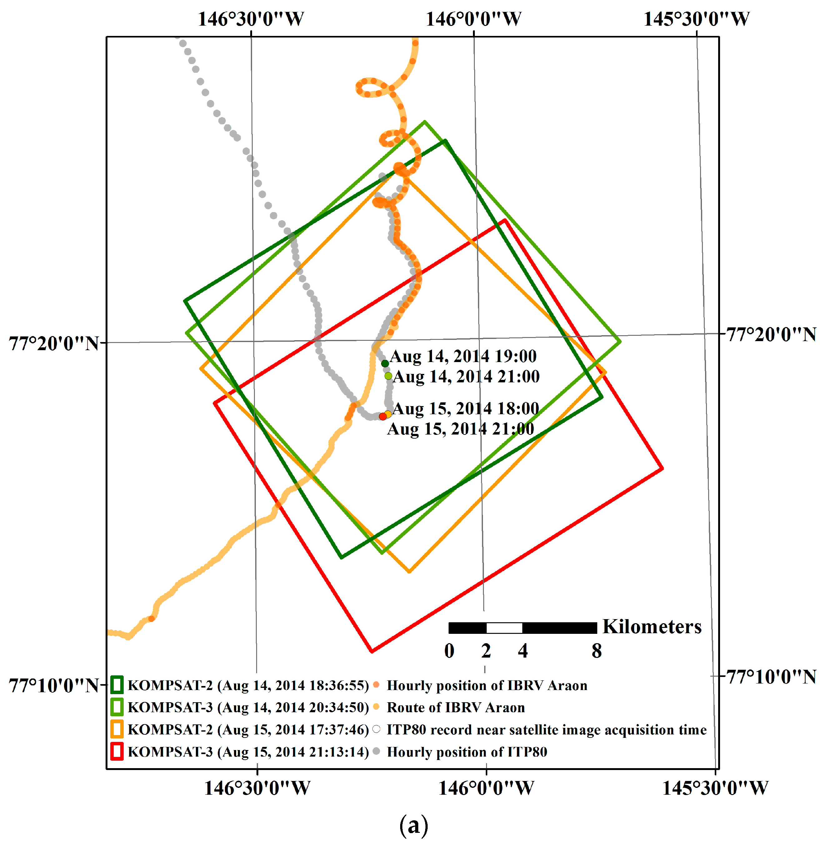
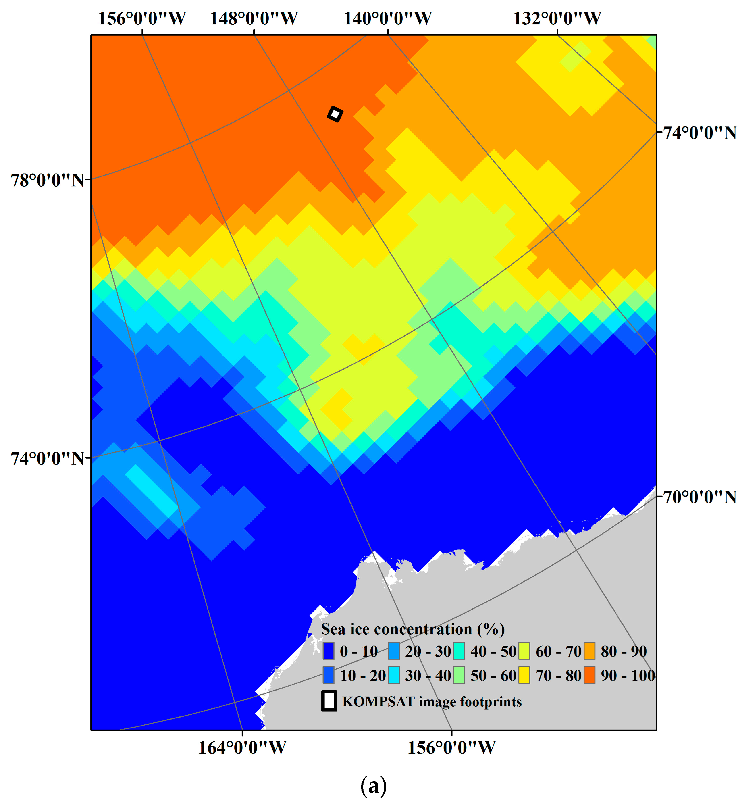
2.1. Description of Study Area
2.2. Acquisition of Dataset
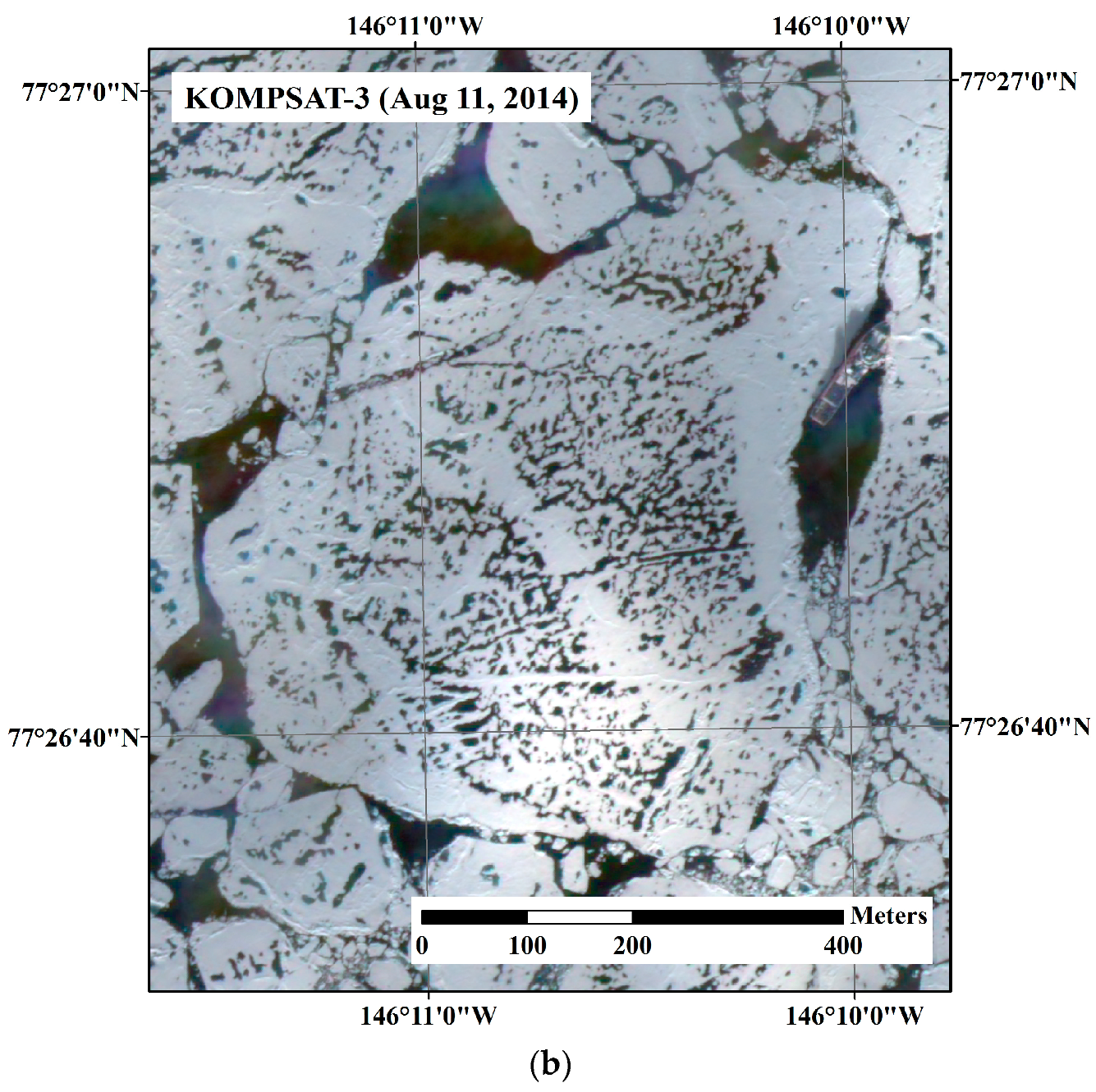
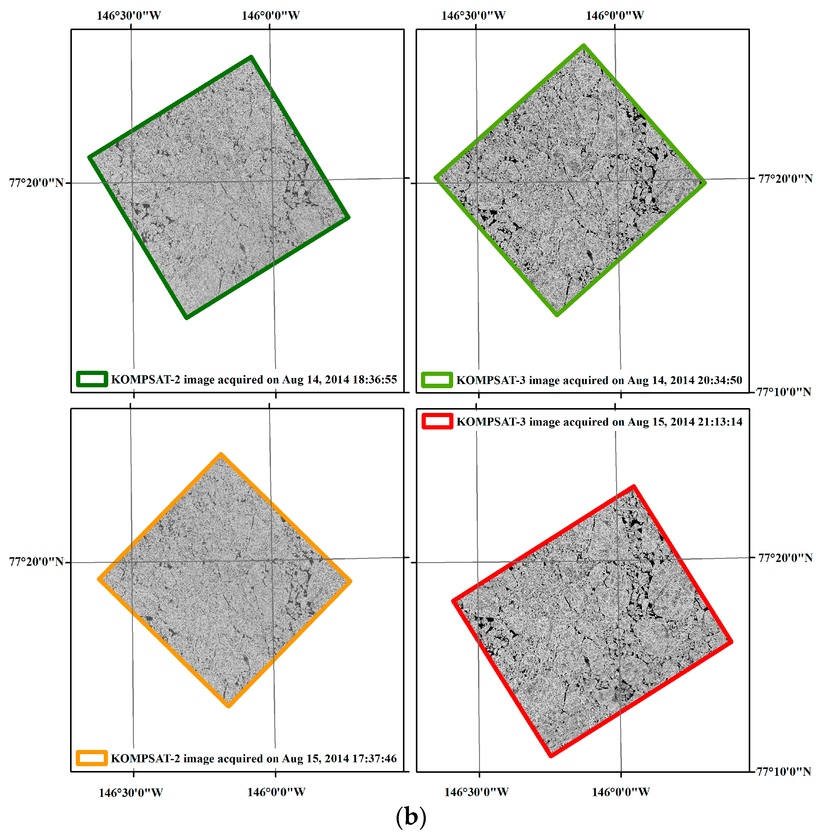
2.2.1. High-Resolution Satellite Image
2.2.2. Ice-Tethered Profiler 80 (ITP80) Buoy Location Record
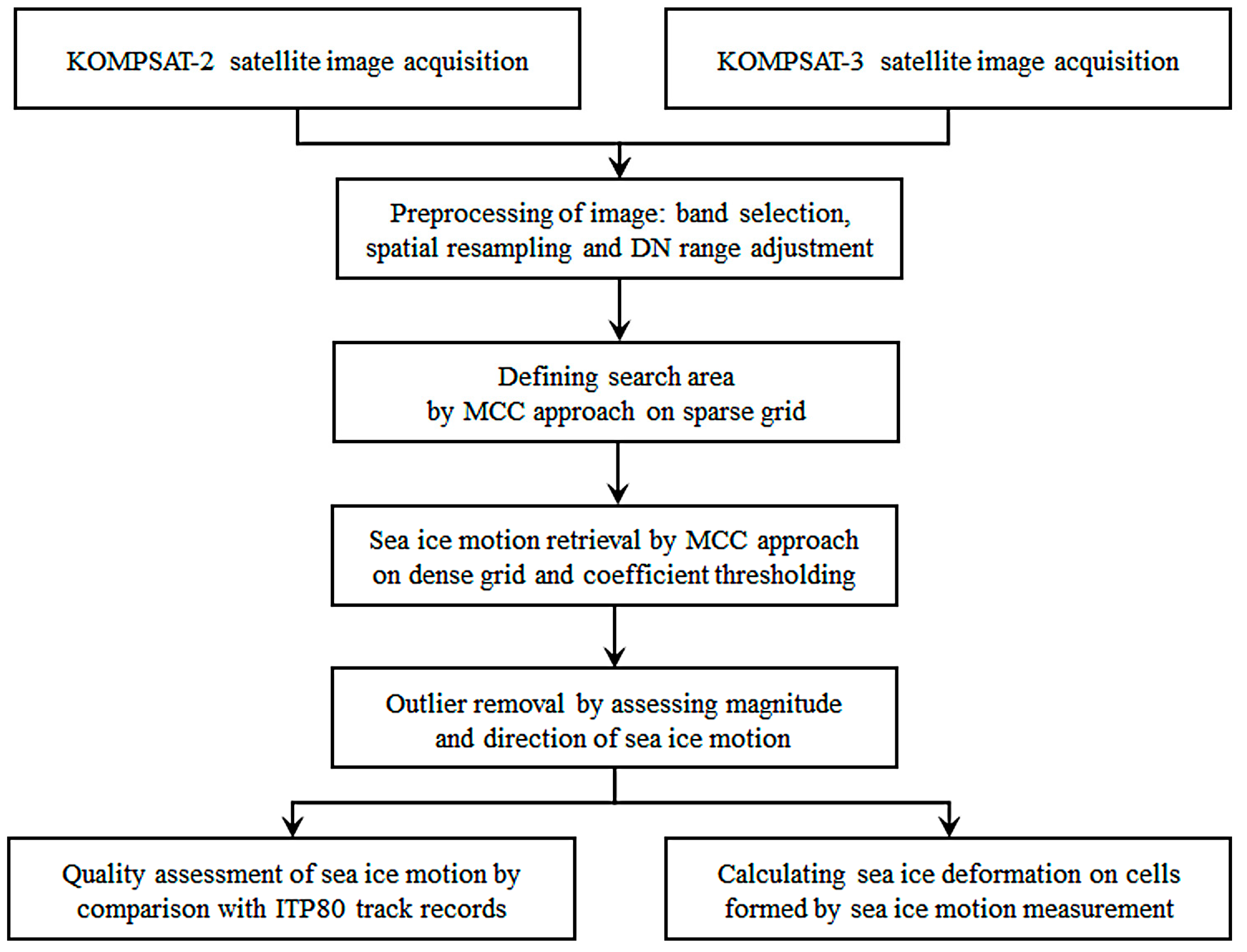
3. Methods
3.1. Measuring Sea Ice Motion and Deformation
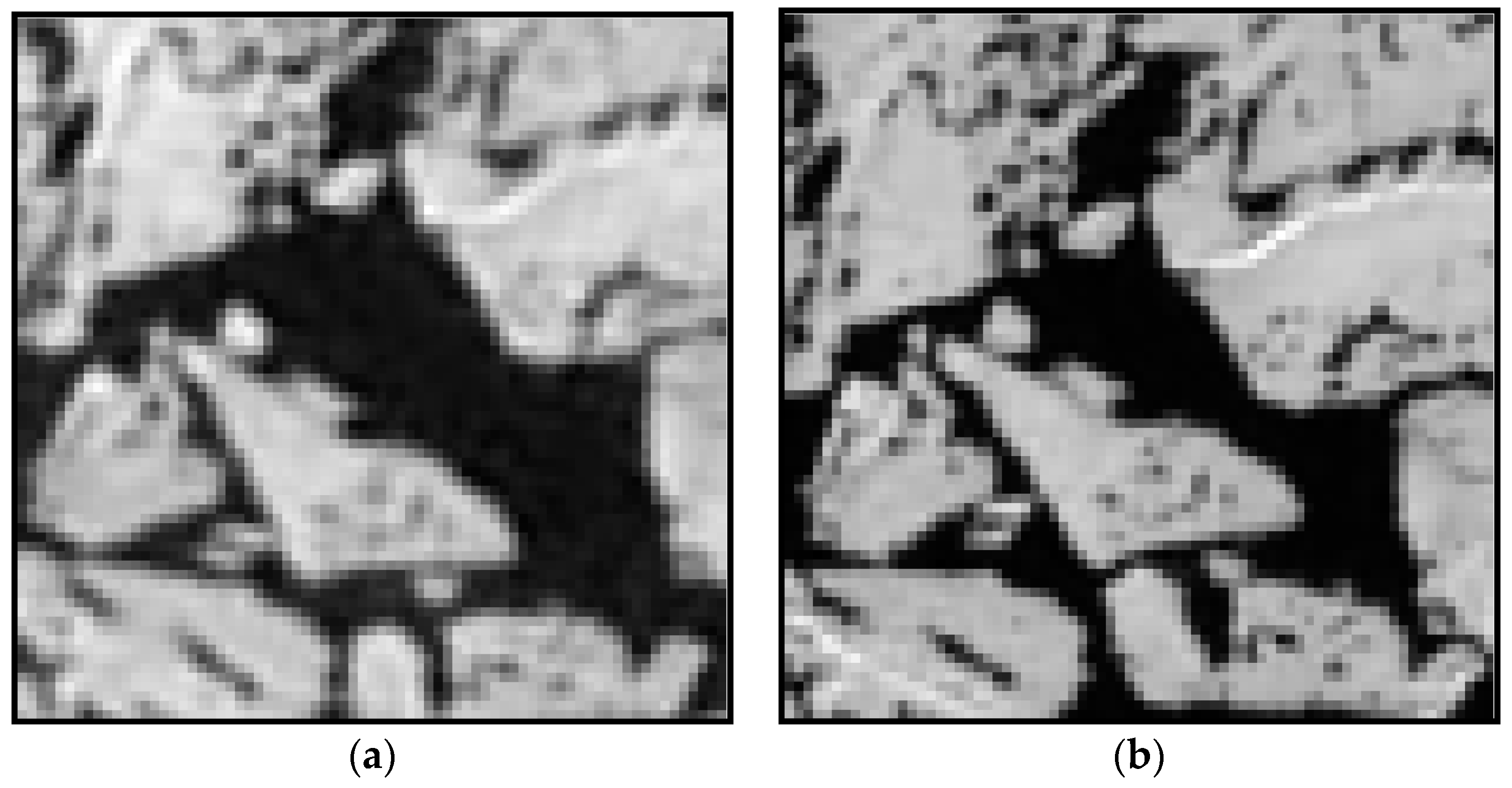
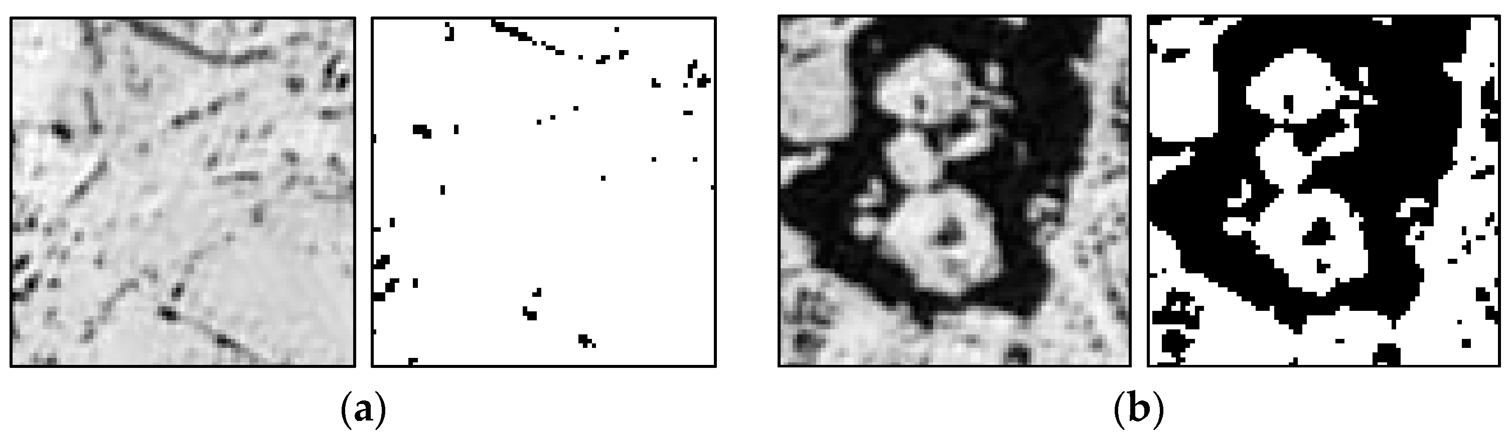
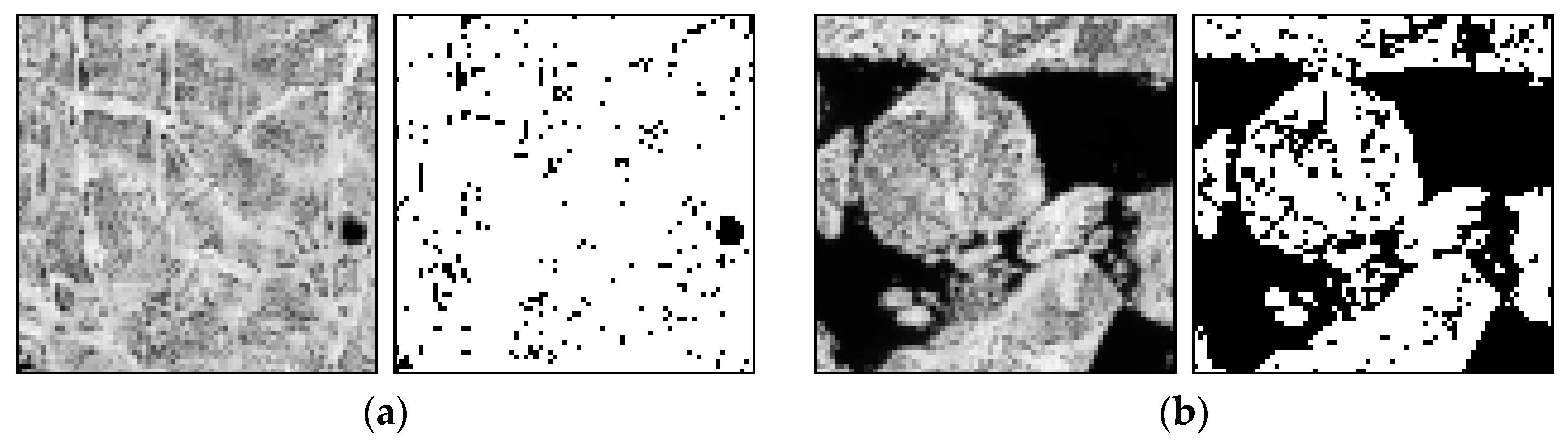
3.1.1. Preprocessing of Satellite Image
3.1.2. Maximum Cross-Correlation Approach for Measuring Sea Ice Motion
3.1.3. Validating Satellite Image-Derived Sea Ice Motion
3.1.4. Measuring Sea Ice Deformation
4. Results
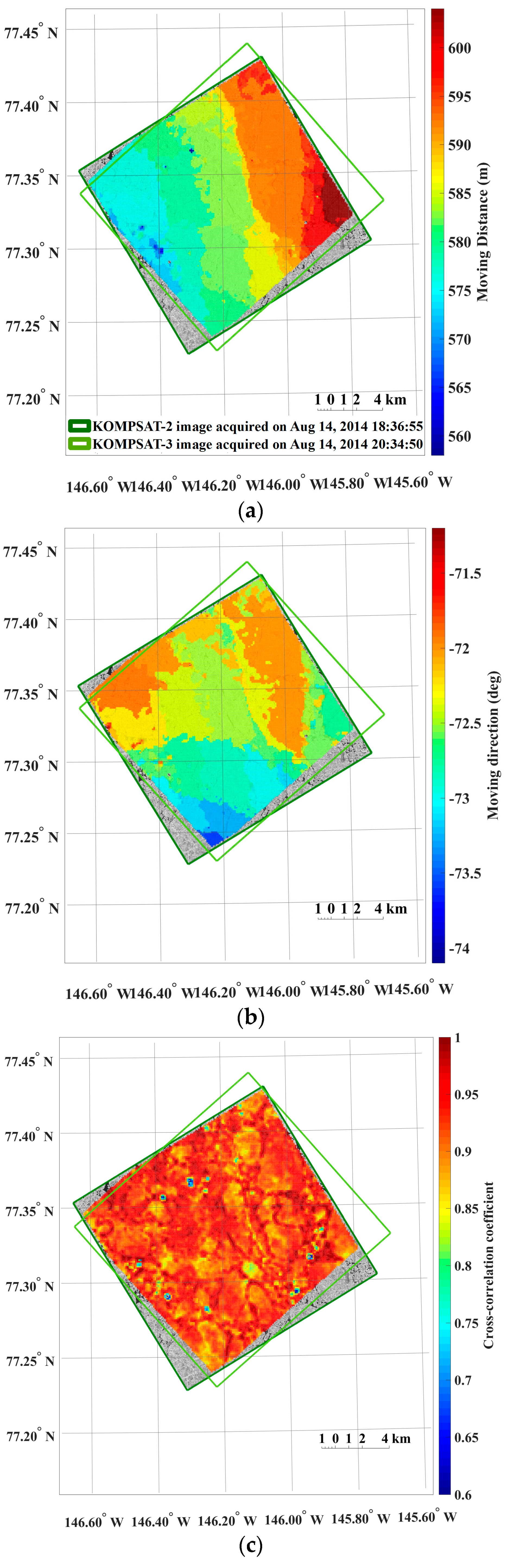
4.1. Sea Ice Motions from Maximum Cross-Correlation Approach
4.2. Quality Assessment of the Sea Ice Motion Measurement
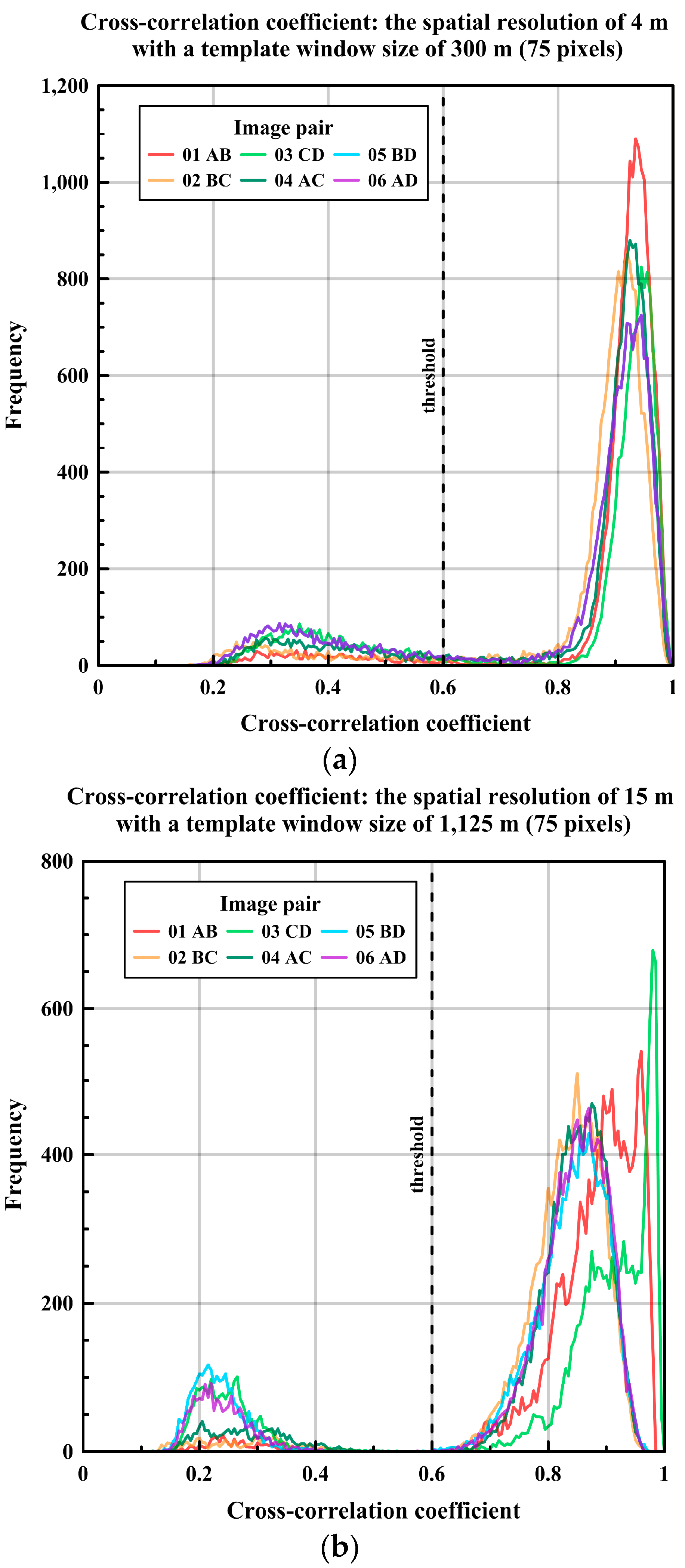
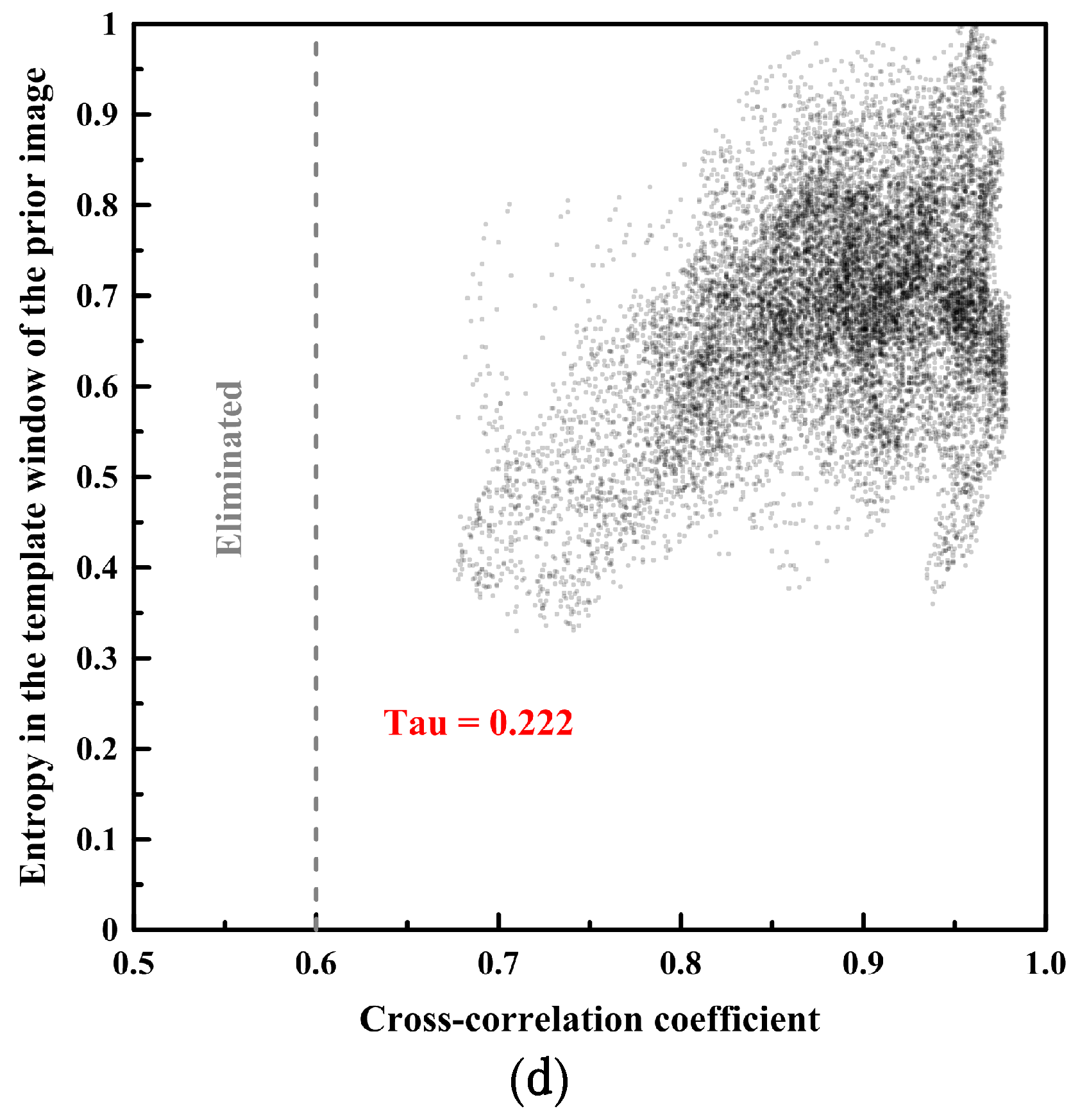
4.3. Relationships Between Cross-Correlation Coefficient and Sea Ice Image Properties
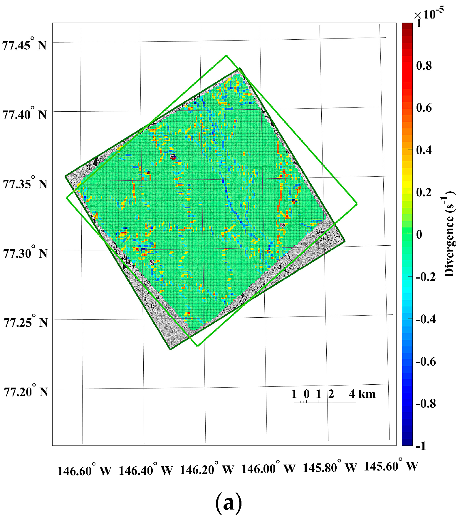
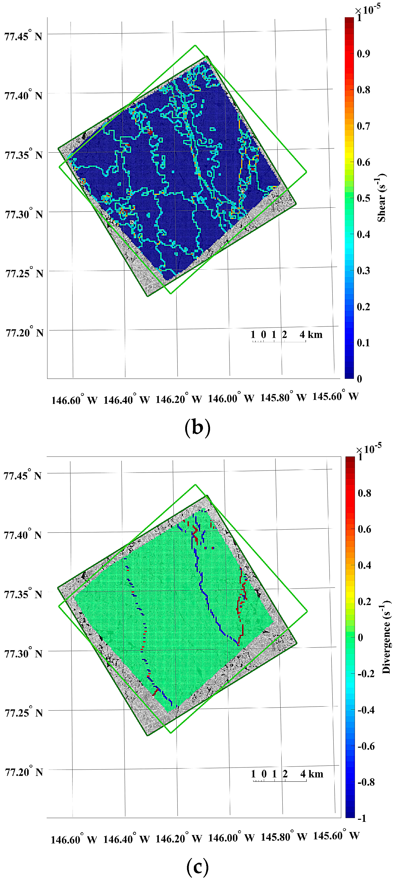
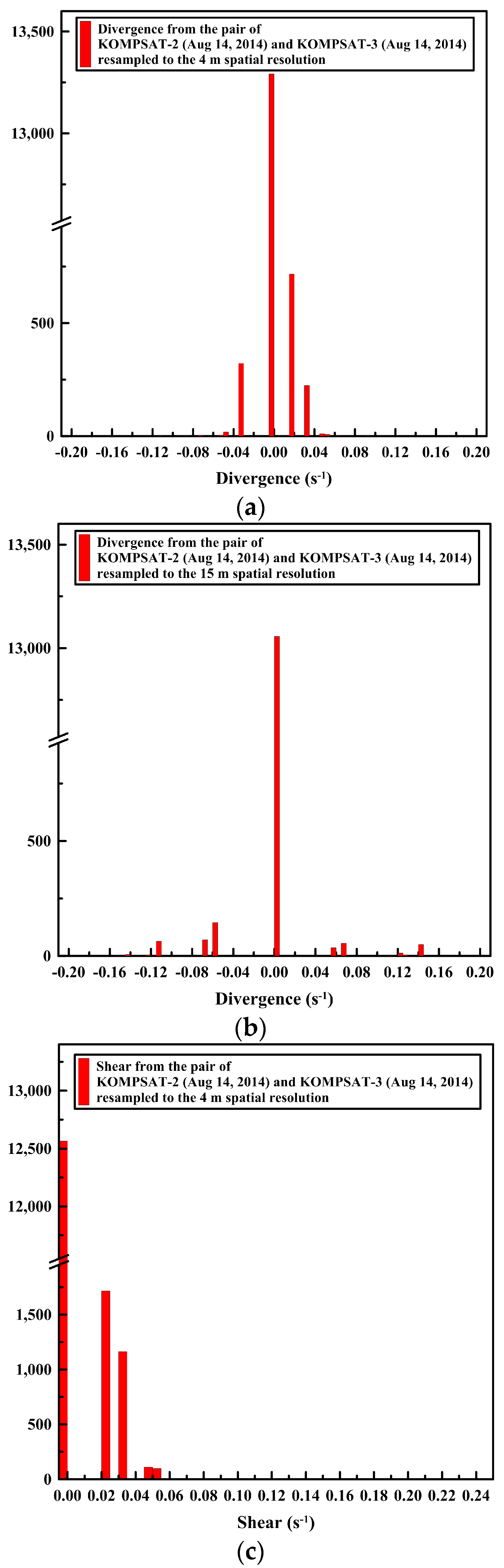
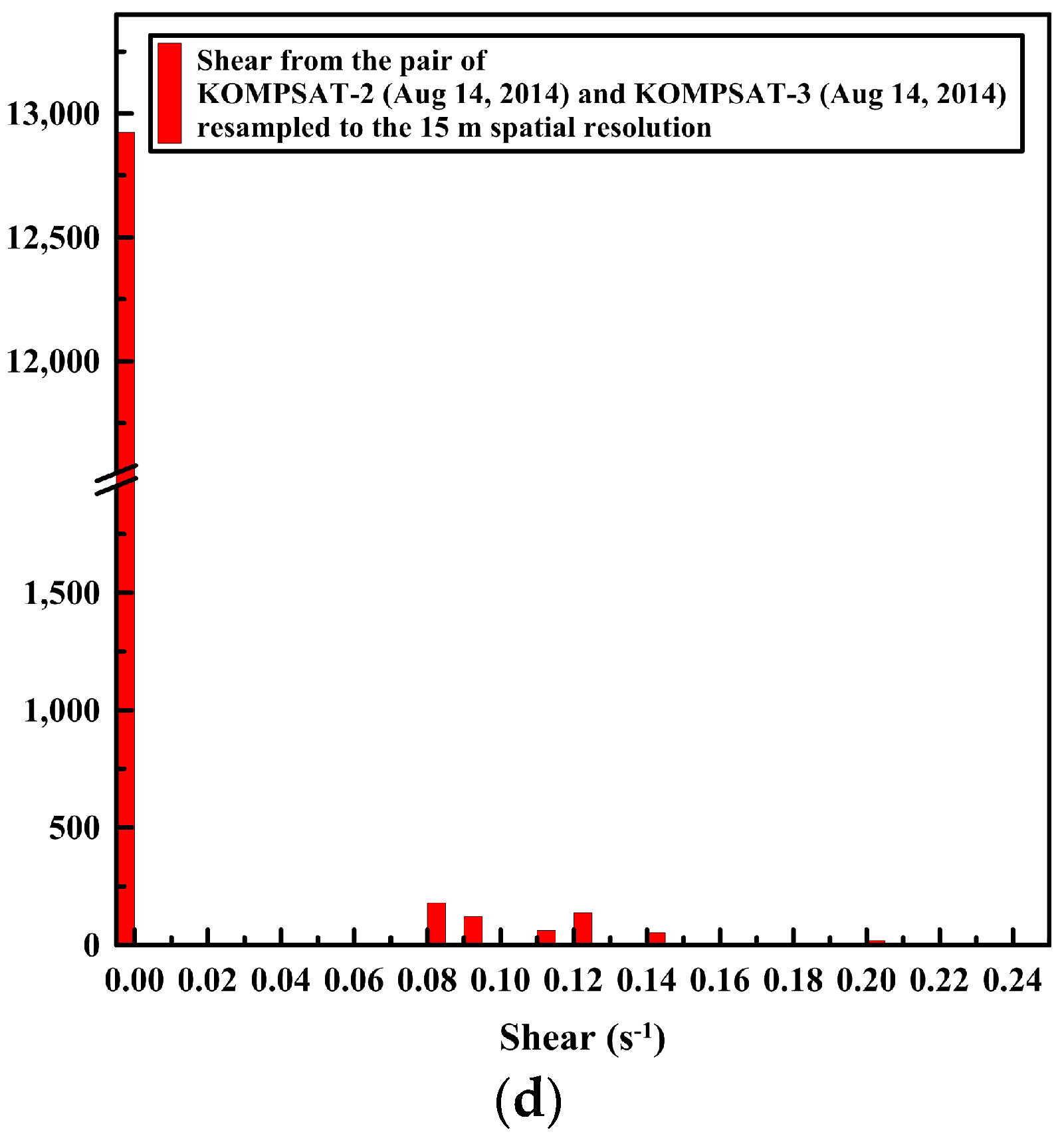
4.4. Sea Ice Deformation
5. Discussion
6. Conclusions
Acknowledgments
Author Contributions
Conflicts of Interest
References
- Heil, P.; Fowler, C.; Maslanik, J.; Emery, W.; Allison, I. A comparison of East Antarctic sea-ice motion derived using drifting buoys and remote sensing. Ann. Glaciol. 2001, 33, 139–144. [Google Scholar] [CrossRef]
- Emery, W.; Fowler, C.W.; Maslanik, J. Satellite-derived maps of Arctic and Antarctic sea ice motion: 1988 to 1994. Geophys. Res. Lett. 1997, 24, 897–900. [Google Scholar] [CrossRef]
- Martin, T.; Augstein, E. Large-scale drift of arctic sea ice retrieved from passive microwave satellite data. J. Geophys. Res. Oceans 2000, 105, 8775–8788. [Google Scholar] [CrossRef]
- Lavergne, T.; Eastwood, S.; Teffah, Z.; Schyberg, H.; Breivik, L.A. Sea ice motion from low-resolution satellite sensors: An alternative method and its validation in the arctic. J. Geophys. Res. Oceans 2010, 115. [Google Scholar] [CrossRef]
- Holland, P.R.; Kwok, R. Wind-driven trends in Antarctic sea-ice drift. Nat. Geosci. 2012, 5, 872–875. [Google Scholar] [CrossRef]
- Kimura, N.; Nishimura, A.; Tanaka, Y.; Yamaguchi, H. Influence of winter sea-ice motion on summer ice cover in the arctic. Polar Res. 2013, 32. [Google Scholar] [CrossRef]
- Yu, J.; Liu, A.; Yang, Y.; Zhao, Y. Analysis of sea ice motion and deformation using AMSR-E data from 2005 to 2007. Int. J. Remote Sens. 2013, 34, 4127–4141. [Google Scholar] [CrossRef]
- Emery, W.J.; Fowler, C.W.; Hawkins, J.; Preller, R.H. Fram strait satellite image-derived ice motions. J. Geophys. Res. Oceans 1991, 96, 4751–4768. [Google Scholar] [CrossRef]
- Vincent, R.; Marsden, R.; McDonald, A. Short time-span ice tracking using sequential AVHRR imagery. Atmos.-Ocean 2001, 39, 279–288. [Google Scholar] [CrossRef]
- Kwok, R. The RADARSAT geophysical processor system. In Analysis of SAR Data of the Polar Oceans; Springer: New York, NY, USA, 1998; pp. 235–257. [Google Scholar]
- Flocco, D.; Laxon, S.; Feltham, D.; Haas, C. Validation and interpretation of a new sea ice GlobIce dataset using buoys and the CICE sea ice model. In Proceedings of the EGU General Assembly, Vienna, Austria, 22–27 April 2012; p. 3174. [Google Scholar]
- Giles, A.; Massom, R.; Heil, P.; Hyland, G. Semi-automated feature-tracking of East Antarctic sea ice from Envisat ASAR imagery. Remote Sens. Environ. 2011, 115, 2267–2276. [Google Scholar] [CrossRef]
- Komarov, A.S.; Barber, D.G. Sea ice motion tracking from sequential dual-polarization RADARSAT-2 images. IEEE Trans. Geosci. Remote Sens. 2014, 52, 121–136. [Google Scholar] [CrossRef]
- Hollands, T.; Haid, V.; Dierking, W.; Timmermann, R.; Ebner, L. Sea ice motion and open water area at the Ronne Polynia, Antarctica: Synthetic aperture radar observations versus model results. J. Geophys. Res. Oceans 2013, 118, 1940–1954. [Google Scholar] [CrossRef]
- Ninnis, R.; Emery, W.; Collins, M. Automated extraction of pack ice motion from advanced very high resolution radiometer imagery. J. Geophys. Res. Oceans 1986, 91, 10725–10734. [Google Scholar] [CrossRef]
- Kwok, R.; Cunningham, G. Deformation of the arctic ocean ice cover after the 2007 record minimum in summer ice extent. Cold Reg. Sci. Technol. 2012, 76, 17–23. [Google Scholar] [CrossRef]
- Lindsay, R.; Stern, H. The RADARSAT geophysical processor system: Quality of sea ice trajectory and deformation estimates. J. Atmos. Oceanic Technol. 2003, 20, 1333–1347. [Google Scholar] [CrossRef]
- Kwok, R.; Cunningham, G.F.; Hibler, W.D. Sub-daily sea ice motion and deformation from RADARSAT observations. Geophys. Res. Lett. 2003, 30. [Google Scholar] [CrossRef]
- Hutchings, J.; Hibler, W. Small-scale sea ice deformation in the Beauport sea seasonal ice zone. J. Geophys. Res. Oceans 2008, 113. [Google Scholar] [CrossRef]
- Liu, C.-C.; Chang, Y.-C.; Huang, S.; Yan, S.-Y.; Wu, F.; Wu, A.-M.; Kato, S.; Yamaguchi, Y. Monitoring the dynamics of ice shelf margins in polar regions with high-spatial-and high-temporal-resolution space-borne optical imagery. Cold Reg. Sci. Technol. 2009, 55, 14–22. [Google Scholar] [CrossRef]
- Hagen, R.A.; Peters, M.F.; Liang, R.T.; Ball, D.G.; Brozena, J.M. Measuring arctic sea ice motion in real time with photogrammetry. IEEE Geosci. Remote Sens. Lett. 2014, 11, 1956–1960. [Google Scholar] [CrossRef]
- Kwok, R. Declassified high-resolution visible imagery for Arctic sea ice investigations: An overview. Remote Sens. Environ. 2014, 142, 44–56. [Google Scholar] [CrossRef]
- Kwok, R.; Curlander, J.C.; McConnell, R.; Pang, S.S. An ice-motion tracking system at the Alaska SAR facility. IEEE J. Ocean. Eng. 1990, 15, 44–54. [Google Scholar] [CrossRef]
- Hollands, T.; Linow, S.; Dierking, W. Reliability measures for sea ice motion retrieval from synthetic aperture radar images. IEEE J. Sel. Top. Appl. Earth Obs. Remote Sens. 2015, 8, 67–75. [Google Scholar] [CrossRef]
- Hodgson, M.E.; Kar, B. Modeling the potential swath coverage of nadir and off-nadir pointable remote sensing satellite-sensor systems. Cartogr. Geogr. Inf. Sci. 2008, 35, 147–156. [Google Scholar] [CrossRef]
- Seo, D.C.; Yang, J.Y.; Lee, D.H.; Song, J.H.; Lim, H. KOMPSAT-2 direct sensor modeling and geometric calibration/validation. In Proceedings of the International Society for Photogrammetry and Remote Sensing Congress, Beijing, China, 3–11 July 2008. [Google Scholar]
- Choi, J.; Jung, H.-S.; Yun, S.-H. An efficient mosaic algorithm considering seasonal variation: Application to KOMPSAT-2 satellite images. Sensors 2015, 15, 5649–5665. [Google Scholar] [CrossRef] [PubMed]
- Yeom, J.-M.; Hwang, J.; Jin, C.-G.; Lee, D.-H.; Han, K.-S. Radiometric characteristics of kompsat-3 multispectral images using the spectra of well-known surface tarps. IEEE Trans. Geosci. Remote Sens. 2016, 54, 5914–5924. [Google Scholar] [CrossRef]
- Cavalieri, D.; Parkinson, C.; Gloersen, P.; Zwally, H.J. Sea Ice Concentrations from Nimbus-7 SMMR and DMSP SSM/I-SSMIS Passive Microwave Data; Version 1; NASA DAAC at the National Snow and Ice Data Center: Boulder, CO, USA, 1996; Available online: http://dx.doi.org/10.5067/8GQ8LZQVL0VL (accessed on 28 March 2017).
- Overview: Ice-Tethered Profiler. Available online: http://www.whoi.edu/website/itp/ (accessed on 8 October 2016).
- Toole, J.; Krishfield, R.; Proshutinsky, A.; Ashjian, C.; Doherty, K.; Frye, D.; Hammar, T.; Kemp, J.; Peters, D.; Timmermans, M.L. Ice-tethered profilers sample the upper arctic ocean. Eos Trans. Am. Geophys. Union 2006, 87, 434–438. [Google Scholar] [CrossRef]
- Krishfield, R.; Toole, J.; Proshutinsky, A.; Timmermans, M.-L. Automated ice-tethered profilers for seawater observations under pack ice in all seasons. J. Atmos. Ocean. Technol. 2008, 25, 2091–2105. [Google Scholar] [CrossRef]
- Rösel, A.; Kaleschke, L. Comparison of different retrieval techniques for melt ponds on Arctic sea ice from Landsat and MODIS satellite data. Ann. Glaciol. 2011, 52, 185–191. [Google Scholar] [CrossRef]
- Zhang, Q.; Skjetne, R. Image techniques for identifying sea-ice parameters. Model. Identif. Control 2014, 35, 293–301. [Google Scholar] [CrossRef]
- Otsu, N. A threshold selection method from gray-level histograms. IEEE Trans. Syst. Man Cybern. 1979, 9, 62–66. [Google Scholar] [CrossRef]
- Gonzalez, R.C.; Woods, R.E.; Eddins, S.L. Digital Image Processing Using MATLAB; Prentice Hall: Upper Saddle River, NJ, USA, 2003; pp. 287–288. [Google Scholar]
- Kwok, R.; Schweiger, A.; Rothrock, D.; Pang, S.; Kottmeier, C. Sea ice motion from satellite passive microwave imagery assessed with ERS SAR and buoy motions. J. Geophys. Res. Oceans 1998, 103, 8191–8214. [Google Scholar] [CrossRef]
- Kwok, R. Ross sea ice motion, area flux, and deformation. J. Clim. 2005, 18, 3759–3776. [Google Scholar] [CrossRef]
- Schwegmann, S.; Haas, C.; Fowler, C.; Gerdes, R. A comparison of satellite-derived sea-ice motion with drifting-buoy data in the Weddell Sea, Antarctica. Ann. Glaciol. 2011, 52, 103–110. [Google Scholar] [CrossRef]
- Hwang, B. Inter-comparison of satellite sea ice motion with drifting buoy data. Int. J. Remote Sens. 2013, 34, 8741–8763. [Google Scholar] [CrossRef]
- Sumata, H.; Kwok, R.; Gerdes, R.; Kauker, F.; Karcher, M. Uncertainty of Arctic summer ice drift assessed by high-resolution SAR data. J. Geophys. Res. Oceans 2015, 120, 5285–5301. [Google Scholar] [CrossRef]
- Notarstefano, G.; Poulain, P.-M.; Mauri, E. Estimation of surface currents in the Adriatic sea from sequential infrared satellite images. J. Atmos. Ocean. Technol. 2008, 25, 271–285. [Google Scholar] [CrossRef]
- Stern, H.L.; Moritz, R.E. Sea ice kinematics and surface properties from RADARSAT synthetic aperture radar during the SHEBA drift. J. Geophys. Res. Oceans 2002, 107. [Google Scholar] [CrossRef]
- Yau, C. R Tutorial with Bayesian Statistics Using OpenBUGS. 2012. Available online: http://www.r-tutor.com/content/r-tutorial-ebook (accessed on 16 March 2017).
- Kwok, R. Satellite remote sensing of sea-ice thickness and kinematics: A review. J. Glaciol. 2010, 56, 1129–1140. [Google Scholar] [CrossRef]
- Tschudi, M.; Fowler, C.; Maslanik, J.; Stroeve, J. Tracking the movement and changing surface characteristics of Arctic sea ice. IEEE J. Sel. Top. Appl. Earth Obs. Remote Sens. 2010, 3, 536–540. [Google Scholar] [CrossRef]
- Centurioni, L. Observations of large-amplitude nonlinear internal waves from a drifting array: Instruments and methods. J. Atmos. Ocean. Technol. 2010, 27, 1711–1731. [Google Scholar] [CrossRef]
- SIIS (SI Imaging Services). Location Accuracy of KOMPSAT Products: DEC. 2014. Available online: http://www.si-imaging.com/lfile/Geolocation (accessed on 3 August 2016).
- Kwok, R.; Sulsky, D. Arctic Ocean sea ice thickness and kinematics: Satellite retrievals and modeling. Oceanography 2010, 23, 134–143. [Google Scholar] [CrossRef]


| KOMPSAT-2 | KOMPSAT-3 | |
|---|---|---|
| Date of launch | 28 July 2006 | 17 May 2012 |
| Main payload | MSC (Multispectral Camera) | AEISS (Advanced Earth Imaging Sensor System) |
| Orbit height | 685 km | 685 km |
| Spatial resolution | 1.0 m Pan and 4.0 m MS | 0.7 m Pan and 2.8 m MS |
| Spectral bands | 500–900 nm PAN | 450–900 nm PAN |
| 450–520 nm MS1 (blue) | 450–520 nm MS1 (blue) | |
| 520–600 nm MS2 (green) | 520–600 nm MS2 (green) | |
| 630–690 nm MS3 (red) | 630–690 nm MS3 (red) | |
| 760–900 nm MS4 (NIR) | 760–900 nm MS4 (NIR) | |
| Mean local time on ascending node | 10:50 h | 13:30 h |
| Data quantization | 10 bit | 14 bit |
| Swath width | 15 km | 16 km |
| ID | Satellite Image | Acquisition Date and Time (UTC) |
|---|---|---|
| A | KOMPSAT-2 MSC | 14 August 2014 18:36:55 |
| B | KOMPSAT-3 AEISS | 14 August 2014 20:34:50 |
| C | KOMPSAT-2 MSC | 15 August 2014 17:37:46 |
| D | KOMPSAT-3 AEISS | 15 August 2014 21:13:14 |
| ITP80 | Specifications |
|---|---|
| Deployed date | 12 August 2014 |
| Deployed location | 77°24.2′N, 146°10.3′W |
| Localization method | GPS positioning |
| Location measurement | Hourly |
| Data processing level | Level 3 |
| Image Pair | Time Interval (hh:mm:ss) | |
|---|---|---|
| 1 | KOMPSAT-2 (14 August 2014)–KOMPSAT-3 (14 August 2014) | 01:57:55 |
| 2 | KOMPSAT-3 (14 August 2014)–KOMPSAT-2 (15 August 2014) | 21:02:56 |
| 3 | KOMPSAT-2 (15 August 2014)–KOMPSAT-3 (15 August 2014) | 03:35:28 |
| 4 | KOMPSAT-2 (14 August 2014)–KOMPSAT-2 (15 August 2014) | 23:00:51 |
| 5 | KOMPSAT-3 (14 August 2014)–KOMPSAT-3 (15 August 2014) | 24:38:24 |
| 6 | KOMPSAT-2 (14 August 2014)–KOMPSAT-3 (15 August 2014) | 26:36:19 |
| Dataset | Parameter | RMSE | Bias |
|---|---|---|---|
| Spatial resolution of 4 m | Displacement | 57.7 m | –11.4 m |
| Velocity | 19.0 m·h−1 | –4.6 m·h−1 | |
| Direction | 4.0° | –1.5° | |
| Spatial resolution of 15 m | Displacement | 60.7 m | –13.5 m |
| Velocity | 18.7 m·h−1 | –4.3 m·h−1 | |
| Direction | 3.8° | –2.0° |
| Image Pair | Correlation Coefficient (Tau) | |||
|---|---|---|---|---|
| Spatial Resolution of 4 m | Spatial Resolution of 15 m | |||
| Cross-Correlation Coefficient vs. Sea Ice Coverage | Cross-Correlation Coefficient vs. Entropy | Cross-Correlation Coefficient vs. Sea Ice Coverage | Cross-Correlation Coefficient vs. Entropy | |
| 1 | −0.341 | 0.338 | −0.221 | 0.222 |
| 2 | −0.200 | 0.195 | −0.166 | 0.166 |
| 3 | −0.287 | 0.277 | −0.026 | 0.026 |
| 4 | −0.233 | 0.230 | −0.193 | 0.193 |
| 5 | −0.121 | 0.116 | −0.236 | 0.237 |
| 6 | −0.235 | 0.231 | −0.258 | 0.258 |
© 2017 by the authors. Licensee MDPI, Basel, Switzerland. This article is an open access article distributed under the terms and conditions of the Creative Commons Attribution (CC BY) license (http://creativecommons.org/licenses/by/4.0/).
Share and Cite
Hyun, C.-U.; Kim, H.-c. A Feasibility Study of Sea Ice Motion and Deformation Measurements Using Multi-Sensor High-Resolution Optical Satellite Images. Remote Sens. 2017, 9, 930. https://doi.org/10.3390/rs9090930
Hyun C-U, Kim H-c. A Feasibility Study of Sea Ice Motion and Deformation Measurements Using Multi-Sensor High-Resolution Optical Satellite Images. Remote Sensing. 2017; 9(9):930. https://doi.org/10.3390/rs9090930
Chicago/Turabian StyleHyun, Chang-Uk, and Hyun-cheol Kim. 2017. "A Feasibility Study of Sea Ice Motion and Deformation Measurements Using Multi-Sensor High-Resolution Optical Satellite Images" Remote Sensing 9, no. 9: 930. https://doi.org/10.3390/rs9090930
APA StyleHyun, C.-U., & Kim, H.-c. (2017). A Feasibility Study of Sea Ice Motion and Deformation Measurements Using Multi-Sensor High-Resolution Optical Satellite Images. Remote Sensing, 9(9), 930. https://doi.org/10.3390/rs9090930