1. Introduction
According to [
1], slums are the most deprived and excluded form of informal settlements. Slums are characterized by poverty and agglomerations of inadequate housing and are often located in hazardous urban areas. In 2016, approximately one in eight individuals lived in a slum. Although there was a decrease from 39% to 30% of urban population living in slums between 2000 and 2014, the absolute number of people living in urban slums continues to grow and it is a critical factor for the persistence of poverty in the world [
2]. Moreover, the urban population of the world’s two poorest regions, South Asia and Sub-Saharan Africa, is expected to double over the next 20 years, which suggests that the slum dwellers in those regions will grow significantly [
1].
There has been a significant increase in the number of studies regarding the usefulness of remote sensing imagery to measure socioeconomic variables [
3,
4,
5,
6]. This trend is partly due to the increasing availability of satellite platforms, advances in methods and the decreasing costs of these images [
7,
8]. Remote sensing imagery may become an alternative source of information in urban settings for which survey data are scarce. In addition, this imagery may complement socioeconomic data that have been obtained from socioeconomic surveys [
3]. The use of remote sensing data to estimate socioeconomic variables is based in the premise that the physical appearance of a human settlement is a reflection of the society that created it and is also based on the assumption that individuals who live in urban areas with similar physical housing conditions have similar social and demographic characteristics [
9,
10].
Slum detection or slum mapping is one of the most recurrent applications in this field of study; scholars have published a minimum of 87 papers in scientific journals over the last 15 years [
8]. These studies have demonstrated that the physical characteristics of slums are distinguishable from the physical characteristics of formal settlements by using remote sensing data [
11,
12,
13]. This is an important area of study because numerous local governments do not fully acknowledge the existence of slums or informal settlements [
1], which hinders the formulation of policies to benefit the poor citizens of cities [
8].
Numerous methods that make use of remote sensing imagery can be used to identify slum areas. Object based image analysis (OBIA) was, until recently, the most used method; other methods include visual interpretation, texture/morphology analysis and machine learning, which is more accurate and is often combined with OBIA [
8]. Machine learning (ML) approaches generally combine textural, spectral and structural features [
12]. The Random Forest classifier (RF) is one of the most popular ML methods for slum extraction that uses very high spatial resolution (VHR) imagery [
12,
14]. Support Vector Machine (SVM) and Neural Networks (NN) are also used for slum identification [
8]. However, most of these ML algorithms are implemented at the pixel level and have limited viability when working with VHR imagery, in contrast to OBIA [
15]. Appropriate ML methods are generally determined by the intuition of the researcher.
According to [
8], most published studies describe the use of remote sensing to map slums and relied on expensive commercial imagery with near-infrared (NIR) information [
16] or three-dimensional data such as LIDAR [
13]. Numerous small cities in developing countries do not have the funds to purchase full satellite imagery and often use RGB data for data extraction via interpretation [
15,
17]. Google Earth (GE) imagery may be the only available source of aerial imagery for small local governments because these images are free to the public [
18,
19]. In addition, Google Earth provides historical VHR imagery for many locations, which may be useful for spatio-temporal urban analysis. According to Google Earth terms of service [
20], GE imagery can be used for non-commercial purposes, and its use is specifically allowed for research papers and other related documents.
The purpose of this study is threefold. First, we explore the possibility of detecting slums within cities by using very high spatial resolution (VHR) RGB GE imagery, image feature extraction and OBIA techniques, without ancillary data. Second, using identical input data, we compare the performance of different ML algorithms to identify slums and determine which algorithm provides the optimal results. Third, we seek to identify a low-cost standardized method to detect slums that is also flexible, easy to automate and may be used in other urban settings with scarce data. We use data for three Latin American cities with different physical and climate conditions and different urban layout characteristics: Buenos Aires (Argentina), Medellin (Colombia), and Recife (Brazil).
The structure of this paper is as follows:
Section 2 describes the methodology including a description of the data and the three classification models that are utilized in this study.
Section 3 provides the results and a discussion of the implemented approach.
Section 4 presents the primary conclusions, suggestions for future research and policy-making implications for local governments and authorities.
2. Methods
Our goal is to design an algorithm that can automatically identify the areas of a city that possess the urban characteristics of a Slum. This problem can be defined as a binary classification problem for which the inputs are features that have been extracted from GE images and the output is a binary variable that assumes the value of 1 if a particular area of the city is a slum and 0 otherwise.
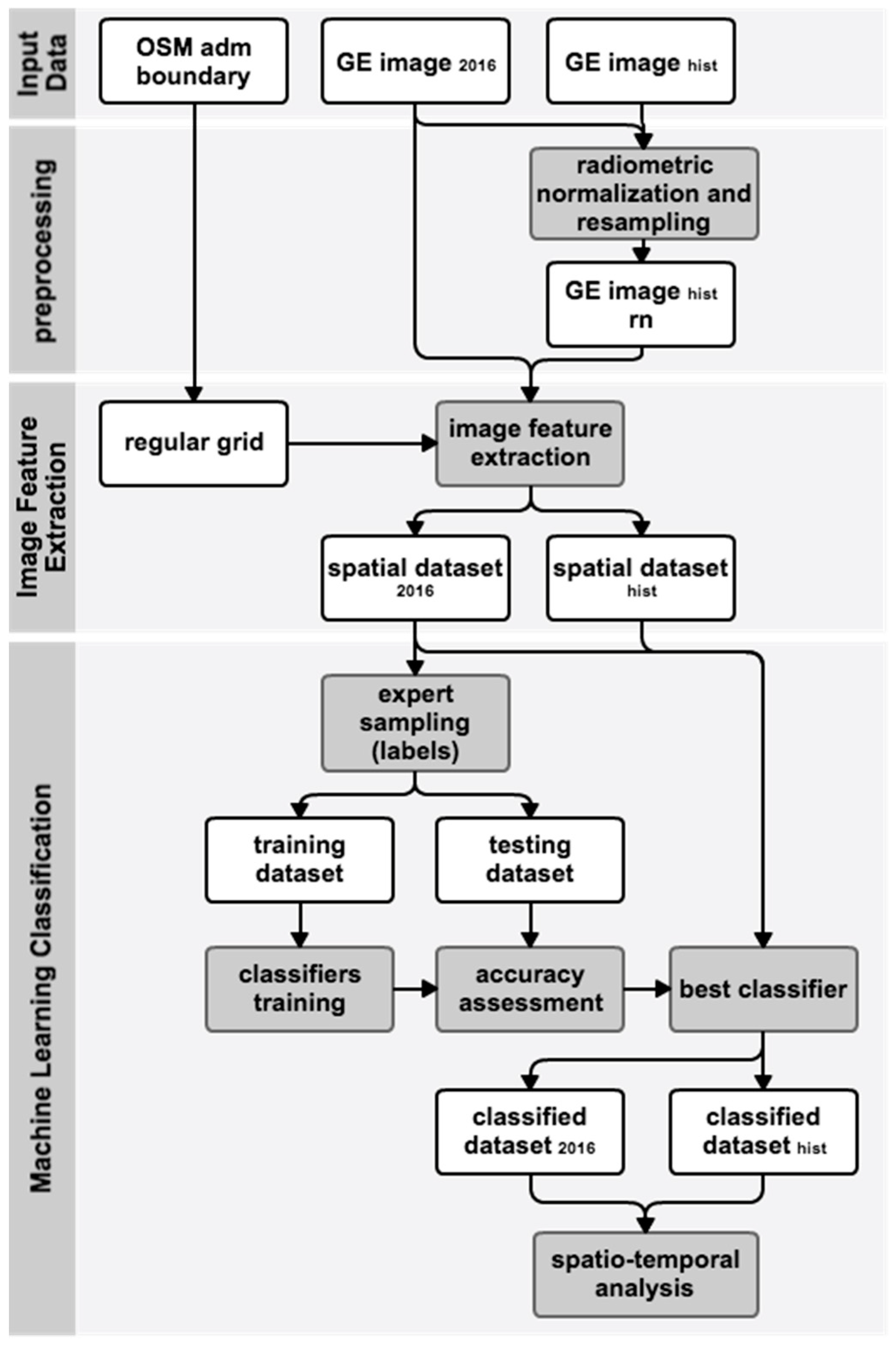
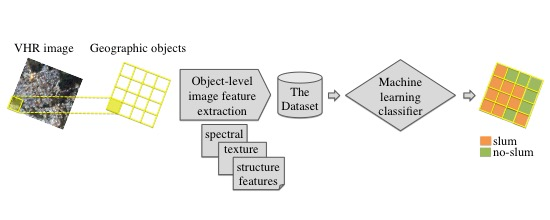
Figure 1 summarizes the proposed approach for detecting slums. This process begins with collecting the input data for the administrative boundaries. Data are obtained from Open Street Maps (OSM) and GE images for two different time instances (upper portion of the figure). The second stage of the process (middle portion of the figure) includes calculating spectral, textural and structural variables (i.e., the image feature extraction) from the GE images. During this stage, the images are discretized by overlapping a regular grid; the outer border is defined by the OSM boundary. This procedure generates Spatial Datasets (one per year, per city) that are composed of regular polygons with their corresponding spectral, textural and structural variables. Finally, the third stage (lower segment of the figure) includes a classification analysis. The data for the most recent year are used to train the classification models and identify the best-performing model for slum identification. The optimal model is then applied to images from prior years to identify urban changes in the most important areas of each city.
2.1. The Data
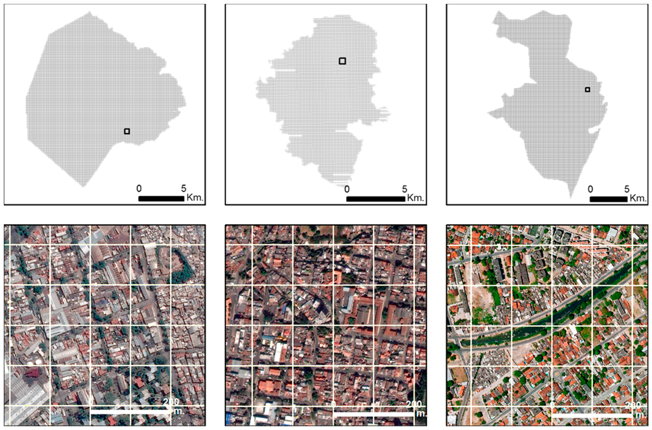
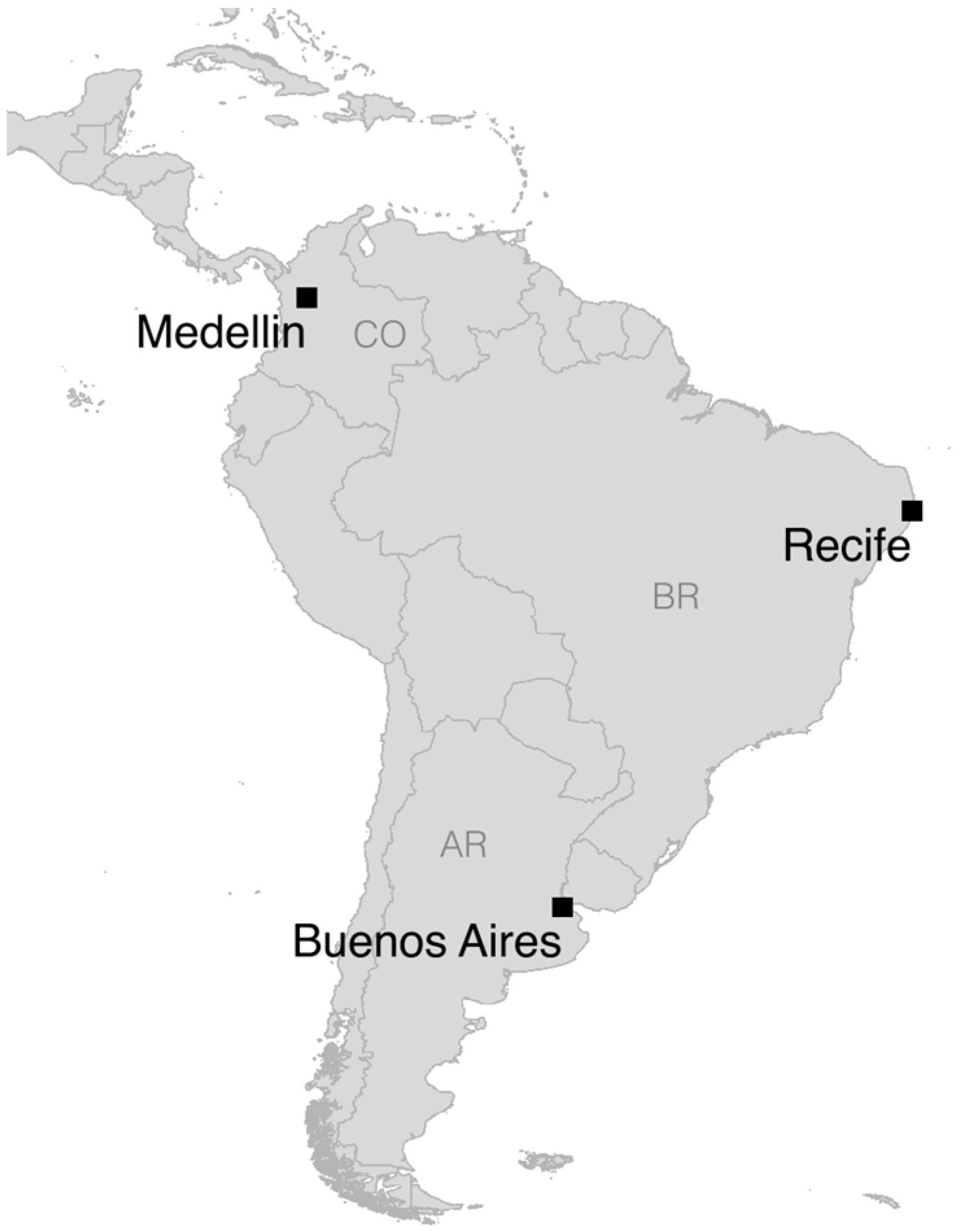
We selected three Latin American cities to test the transferability of this approach: Buenos Aires, Argentina; Medellin, Colombia; and Recife, Brazil (
Figure 2). These cities represent different climates, environmental conditions, and cultures and the use of different building materials. Buenos Aires is located at 34°35′59″ S, 58°22′55″ W at sea level and borders the La Plata river outlet to the ocean over plain lands and has a dry climate with marked seasons. Medellin is located at 6°14′41″ N, 75°34′29″ W in an intermountain valley at 1460 m above mean sea level and has a tropical, wet climate. Recife is located at 8°03′14″ S, 34°52′51″ W at sea level in a hilly terrain and has a tropical, wet climate.
Table 1 provides general descriptions of these cities.
We downloaded the most updated (up to March 2016) GE images for each city and used a zoom level that was similar to VHR imagery with sub-meter pixel size. Google Earth imagery with very high spatial resolution is available for almost all urban areas worldwide. The VHR images were obtained from a number of providers or satellite platforms (e.g., Digital Globe, Geo Eye, and CNES/Astrium, among others). Images are captured by different sensors on different dates using different spatial resolutions; however, most of the images have a submeter pixel size and serve as natural-colored images that have three bands: red, green and blue (RGB). Because of the differences in platforms and different dates of acquisition, images captured at the same location on different dates will indicate differences through illumination conditions and color intensities. The GE images were georeferenced and rescaled between 0 and 255. We kept the preprocessing of the images to a minimum to gain speed in the workflow and to maintain the ease of automation of the whole approach.
Prior studies state that block-level spatial units of analysis are the most useful for urban planning purposes [
13,
24]. OpenStreetMap (OSM) data that layer streets and roads are useful to delineate urban blocks. However, in developing countries, cities’ street networks are incomplete because of the high density and complexity of slum areas [
13] or because areas that have been recently occupied have not been registered in all of the OSM datasets, as is the case for the northeastern section of Medellin city. In these instances, the delineation of urban blocks would add considerable processing time to the approach because it would require visual interpretation and manual digitalization of roads and pedestrian paths.
A simple alternative that can be automated is using a regular grid to detect slums from remote sensing imagery. Prior studies have used regular grids to extract, aggregate and classify image data [
8,
25,
26]. A regular grid in a vector, or fishnet, format can be drawn using any GIS software; the only necessary input is the boundary of the study area. This method could increase the speed of this study. We tested the use of two fishnets with different polygon sizes (a fishnet with square cells of 100 m on each side and another fishnet with square cells of 50 m on each side) for image feature extraction and classification. The results that were obtained with the 100 m grid outperformed the results that were obtained with the 50 m grid in regards to the correct classification of slum-like areas. The 100 m square cells are similar in size to actual urban blocks and have been recognized as an appropriate spatial unit of analysis to study intra-urban poverty for urban planning and policy making [
24]. We downloaded the administrative boundaries of each city from OSM using QGIS [
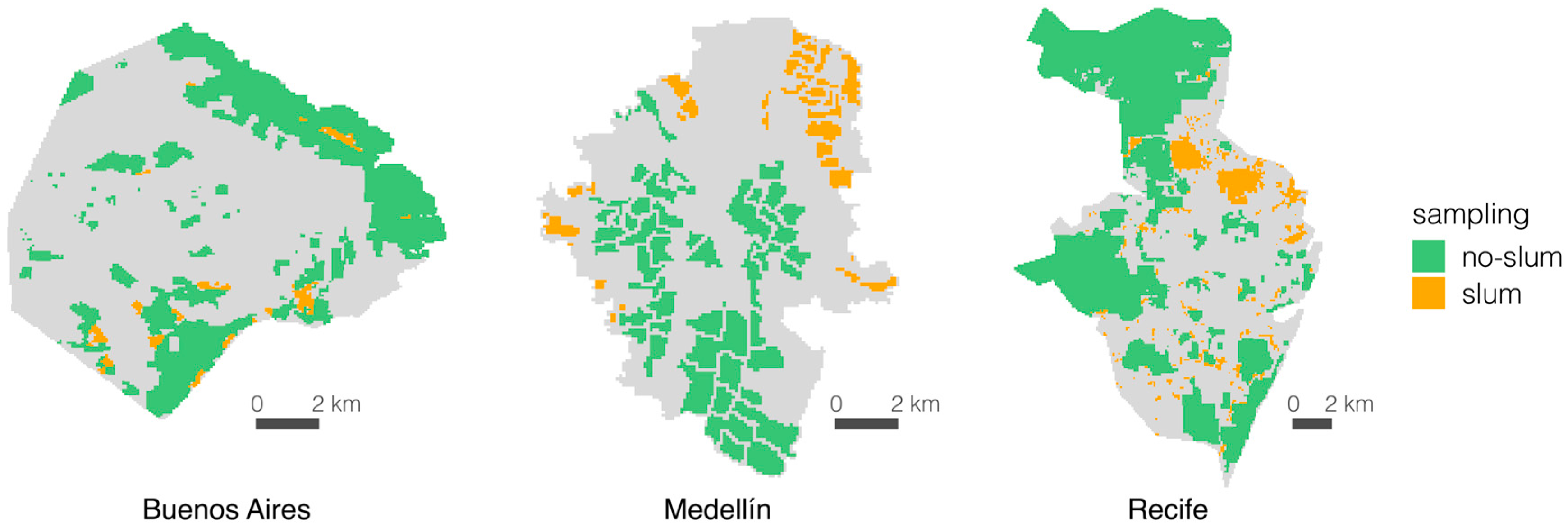
27] to define the extent of the study areas, and then created a regular grid of square cells with 100 m on each side over the urban areas of each city to extract the image features. The use of administrative boundaries to select the study areas could introduce bias in the identification of slums, as those areas located just outside the fringe will not be included in the analysis. As the focus of this work is to test the ability to identify slums from GE imagery in the three different Latin American cities using the same approach, rather than identify all the slum areas in a particular city, we used the administrative boundaries to select the areas in the same way for all three cases.
In addition, we selected well known slum areas in each city and downloaded cloud-free GE images for each sector from approximately a decade prior to test the approach’s ability to analyze changes in slum areas. We attempted to capture images from the same city at two different points in time that were roughly a decade apart to determine if the proposed approach could identify changes that had taken place between the dates. This time span was restricted by the availability of Google Earth’s VHR images for each city and by the quality of the available images, which can be affected by the presence of clouds and shadows. Historical VHR imagery provided by GE is also restricted to the availability of commercial VHR data, which was released after the launch of the Ikonos satellite in 1999. The most updated good quality VHR images available for Buenos Aires, Medellin, and Recife are from 2006, 2008, and 2008, respectively. Although images from other dates are available for these cities in GE, they were captured using medium spatial resolution platforms and are not suitable for extracting spatial pattern descriptors at the intra-urban scale.
The historical GE images were resampled to the identical pixel size of the 2016 images of each city, and we performed radiometric normalization between the historical images and the 2016 images; the 2016 images were used as a reference. Resampling and radiometric normalization were performed to obtain historical images with the identical pixel size and similar color intensity as the 2016 images (i.e., pixel values in each RGB band). Preprocessing the historical images simplifies the process to identify changes and differentiates between changes in intensity because of differences in illumination and atmospheric conditions.
2.1.1. Feature Extraction
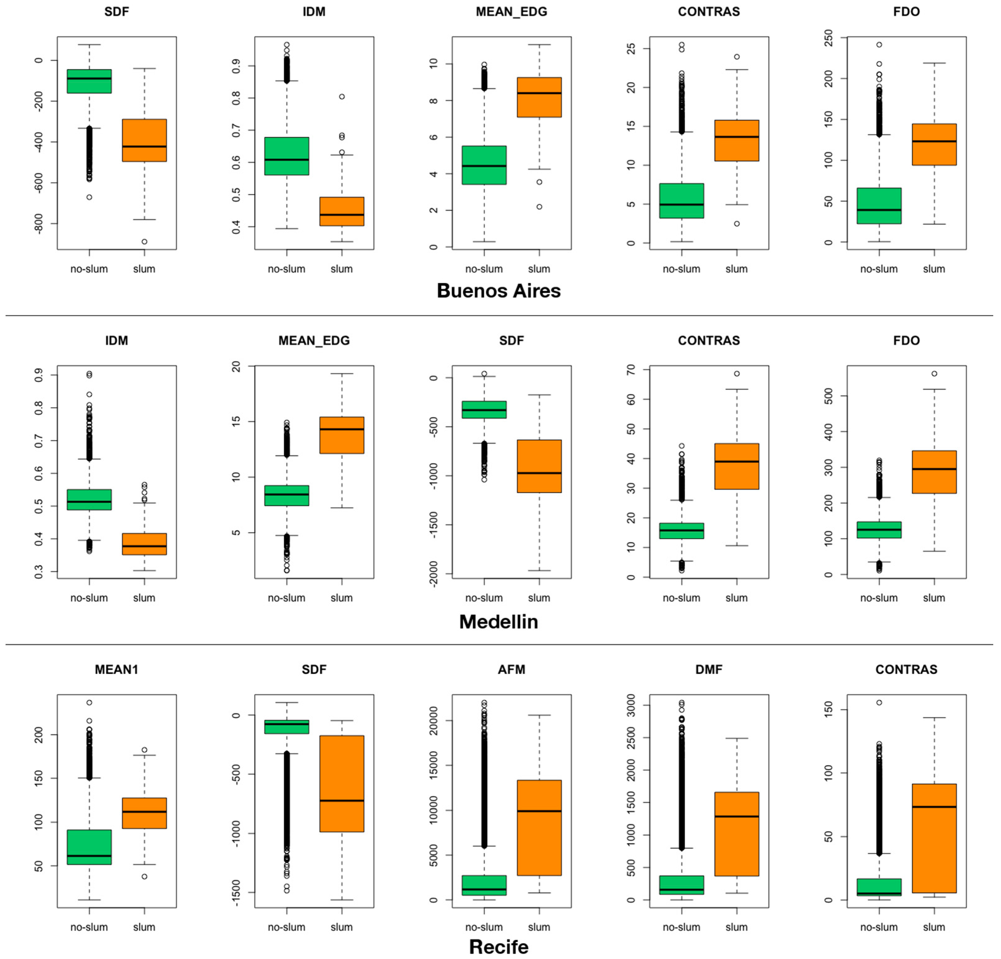
Different image texture measures and spatial pattern descriptors (structure measures) have been used for differentiating slum areas from formal ones in several cities of developing countries around the world [
3,
12,
24,
28,
29]. We used current GE images (obtained in March 2016) and the regular grid of each city to extract image information using FETEX 2.0.
Figure 3 illustrates the outline of the urban areas for each city and selected sectors (500 by 500 m) illustrate the regular grid over the 2016 GE images. FETEX is an interactive software package that is used for image and object-oriented feature extraction [
30] and is available on the Geo-Environmental Cartography and Remote Sensing Research Group website [
31]. We calculated three sets of variables: a set of spectral features, a set of textural features and a set of structural features. The image features are extracted from the image by processing the pixels that are located within the same polygon without changing the image resolution or pixel values. Spectral features provide information regarding color; texture and structural features provide information regarding the spatial arrangement of the elements within the image. The urban layout of slum-like neighborhoods often displays a more organic, crowded and cluttered pattern than for more formal and wealthy neighborhoods. Texture and structural features may help to differentiate between slum and no-slum areas [
3,
12,
32,
33].
Spectral features: Spectral features include the summary statistics of pixel values inside each polygon. These features provide information regarding the spectral response of objects, which differs for land coverage types, states of vegetation, soil composition, building materials, etc. [
30]. We selected the mean and standard deviation for each RGB band and the majority statistic, to be extracted within this group. These features are easy to understand and provide better information about the spectral differences across the cities than other summary statistics (minimum, maximum, range, and sum).
Texture features: Textural features characterize the spatial distribution of intensity values of an image and provide information about contrast, uniformity, rugosity, etc. [
30]. FETEX 2.0 performs texture feature extraction based on the Grey Level Co-occurrence Matrix (GLCM) and a histogram of pixel values inside each polygon. The kurtosis and skewness features are based on a histogram of the pixel values inside the polygon; the GLCM describes the co-occurrences of the pixel values that are separated at a distance of one pixel inside the polygon and is calculated considering the average value of four principal orientations, 0°, 45°, 90° and 135°, to avoid any effects of the orientation of the elements inside the polygon [
30]. The GLCM of FETEX 2.0 was utilized to calculate a set of variables that were proposed by [
34] and are widely used for image processing, including uniformity, entropy, contrast, inverse difference moment (IDM), covariance, variance, and correlation. The edgeness factor is another useful feature that represents the density of the edges of a neighborhood. The mean and standard deviation of the edgeness factor (MEAN EDG, and STDEV EDG) are also computed within this set of texture features in FETEX 2.0 [
30].
Structural features: These features provide information regarding the spatial arrangement of elements inside the polygons in terms of the randomness or regularity of their distribution [
30,
35,
36]. Structural features are calculated in FETEX using the experimental semivariogram approach. According to [
30], the semivariogram quantifies the spatial associations of the values of a variable, measures the degree of spatial correlation between the different pixels of an image and is a suitable tool to determine regular patterns. FETEX 2.0 obtains the experimental semivariogram for each polygon by computing the mean of the semivariogram calculated in six different directions, from 0° to 150° in increments of 30°. Then, each semivariogram curve is smoothed using a Gaussian filter to reduce experimental fluctuations [
30]. Structural features extracted from the semivariogram are based on the zonal analysis that is defined by a set of singular points on the semivariogram, such as the first maximum, the first minimum, and the second maximum [
30]. For a full description of these features, see [
30,
35,
36].
Table 2 provides a list of the remote sensing variables that are used for this analysis.
2.1.2. The Dataset
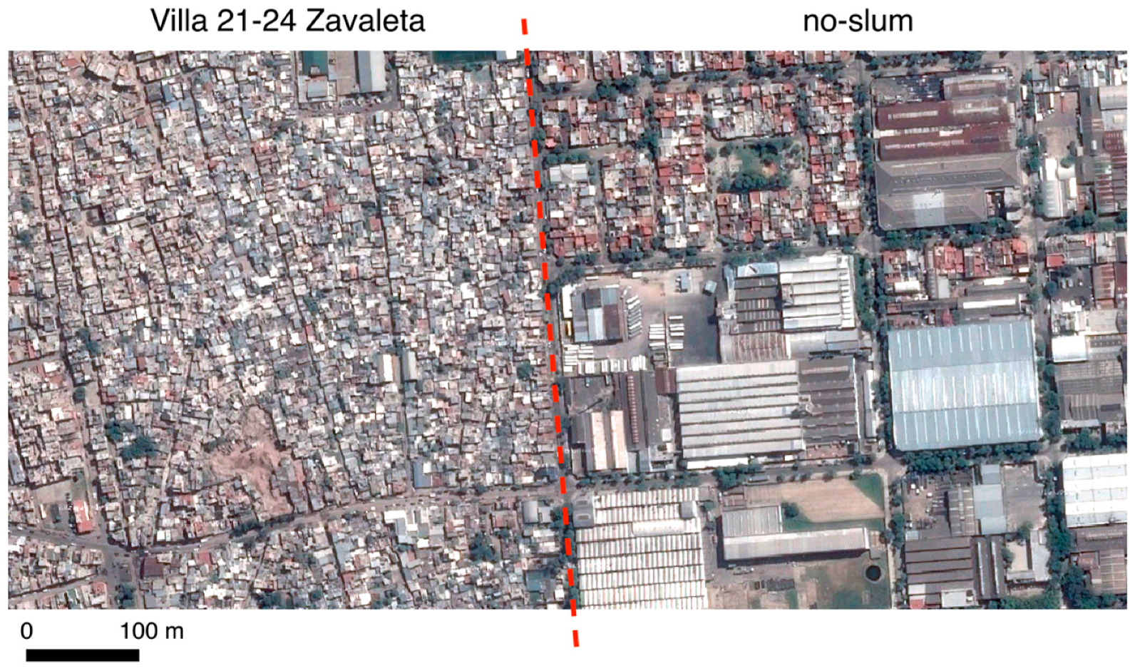
After the image features are extracted, the next step is to create the dataset. This process includes selecting a ground truth sample for each city. Each polygon of the sample is manually labeled as one of two categories: slum or no-slum. Ancillary information and prior studies were used as reference to identify slum areas in each city for sampling. A slum area can be considered a homogeneous zone with specific characteristics, but it can exhibit different appearances depending on the context [
37]. However, most slum definitions relate to physical aspects of the built environment, which makes them comparable across settings. Although each city could have its own definition of slum, as pointed out by Taubenböck and Kraff, “the term slum is difficult to define, but if we see one, we know it” ([
13], p. 15). The location of slum areas in Buenos Aires were identified on the “Caminos de la Villa” website [
38] that provides an interactive map of the city and the location of recognized “villas” (slums). For Medellin we used the delineation of urban slums from [
3,
39], which is based on survey data and the UN-Habitat global definition of slum [
40]. The benchmark slum areas in Recife were identified using the work of [
41], which shows the delimitation of widely recognized slum areas or “favelas” in that city. We visually checked the selected slum areas in each case to ensure that we were picking similar slum-like areas in all three cities. We then labeled as “slum” all the 100 m cells that overlapped with the slum areas from those already identified in the benchmarks. The sampling of no-slum areas in each city included different formal urban layouts such as high and low rise residential areas, parks, urban forests, green spaces, and commercial and industrial areas such as malls, transport facilities and factories. This binary classification scheme is common practice in remote sensing object-oriented approaches for identifying slum areas [
13,
28,
29]. When benchmark information of slum areas is not available to construct a ground truth sample, practitioners must find reference information from local authorities or use an experienced interpreter who can visually determine slum and no-slum areas.
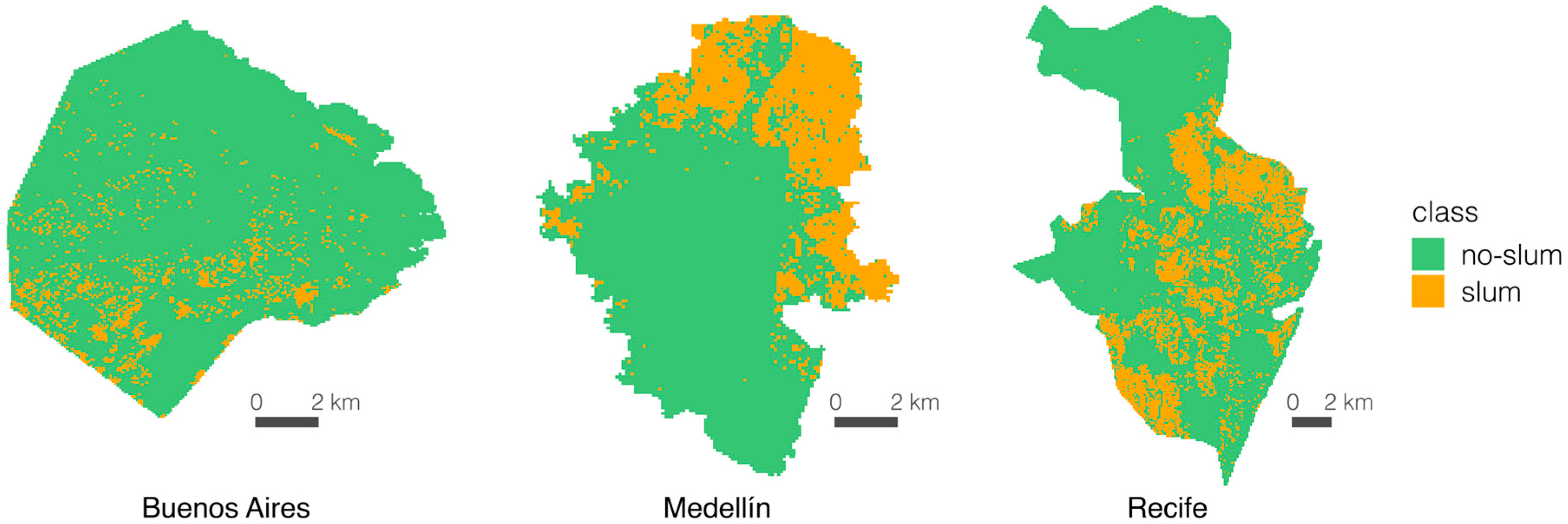
Figure 4 provides the sampling spatial distribution for each city.
The final step in this stage is to divide the dataset into two sets: the training set that includes 60% of the sampled polygons for training and tuning the classification models and the testing set that includes 40% of the sampled polygons to evaluate the predictive capability of the classification models.
Table 3 summarizes the composition of the datasets.
After the ground truth sampling was complete, we used the Kolmogorov–Smirnov (KS) test [
42] and implemented the R package “kolmin” [
43,
44] to better understand the discriminating ability of the image-derived variables to differentiate slum areas from no-slum areas in each city.
2.2. Classification Model
Classification literature is broad and multiple methods and algorithms have been proposed over recent decades [
45]. In general, the primary goal is to develop a quantitative classification method that is capable of determining and generalizing the relationships between a set of variables (
X) and a categorical variable (
Y). For our specific classification problem,
X is a matrix that includes the spectral, textural, and structural values of each polygon in the grid and
Y is a categorical variable that assumes the value of either 1 or −1 if a polygon is a slum or no-slum, respectively. The capability of the classification method is determined by two factors: (i) the theoretical definition of the classification boundary of the classifier (e.g., linear and nonlinear); and (ii) the complexity of the data.
Based on the classification boundary, classifiers are commonly designated as either linear or nonlinear. Linear classifiers, such as logistic regression and linear SVMs, assume that the categorical variable (
Y) can be obtained by exploiting a linear combination of the input features (
X). Nonlinear classifiers generalize the boundary by adjusting polynomial boundaries, Gaussian kernels, or algorithmic criteria based on feature thresholding.
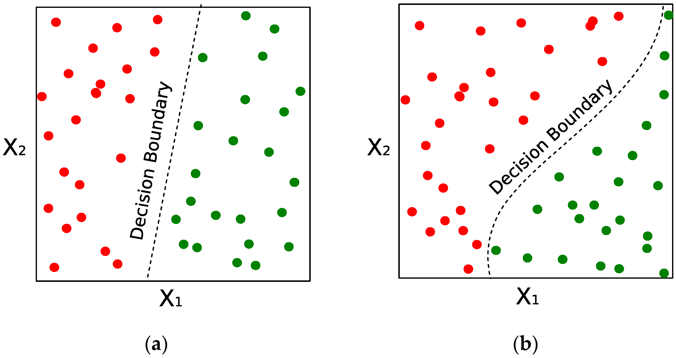
Figure 5 illustrates a linear and nonlinear decision boundary. Nonlinear classifiers can capture more complex patterns from the data, but as a consequence, are more computationally complex than their linear counterparts and may be able to memorize the training data (overfitting).
The intrinsic complexity of the data cannot be easily understood or described, particularly for high dimensional datasets. The most intuitive method to understand the data complexity is by visualizing its features and the respective classes. This approach is generally restricted to low dimensional data (2D or 3D) or simplified versions of the feature space that are obtained using manifold algorithms such as Principal Components Analysis (PCA), IsoMaps, or Self Organizing Maps [
46]. A common approach that is used when working with dimensional data is to determine its complexity by comparing the capabilities of different classification algorithms to capture known patterns. To clarify, a simple classifier (linear) will perform poorly when using complex data (nonlinear) and complex classifiers (nonlinear) are able to use more complex data but have a large risk of overfitting. This risk is referred to as the bias–variance tradeoff [
47], and it is commonly faced by adding a theoretical strategy known as regularization. The regularization strategy depends on the classification method and goes from the inclusion of additional terms in the error functions (e.g., Logistic Regression, SVM) to random disturbances in the training step and/or training data (e.g., Deep Neural Networks). In regards to the size of the training sets, there is no definitive number of observations that are required to train the models; this issue is commonly noted as a consequence of the complexity of the problem that is to be solved. Recent advances in data-science and deep-learning frequently refer to the benefits of large datasets; however, when data collection is expensive and time-consuming, a common practice is to observe changes in the evaluation criteria and sequentially increase the number of observations that are used to train the models. If the evaluation criteria do not improve (converge) as the number of training samples increases, then it is not necessary to collect additional training data.
Because our data have high dimensionality (30 features extracted per polygon) with unknown distributions and include data for three different cities, we explored two approaches for training our model to identify slums: (i) train a unique classifier on an unified dataset (i.e., without differentiating the cities) and then evaluate if the resulting slums are reliable; and (ii) use a multi-model approach by training the classifier in each city. Given the geographic and cultural differences as well as in the appearance of slums in these cities, fitting one method for slum identification in all the cities is a huge challenge. However, it is important to test its feasibility in the search of robust tools for rapid urban slum detection with good performance in different settings. We analyze the performance of linear (Logistic Regression, linear SVM) and nonlinear classifiers (Polynomial and Radial Basis Kernel SVMs and Random Forests), which are available in the Python library Scikit-learn by [
48].
The Logistic Regression (LR) is the most common linear classifier and is frequently used by policy makers in the econometric literature. This classifier is a mathematical approach whose primary goal is to use the logistic function to estimate the probability of a categorical value,
Y, given the input features,
X. For this classifier we used the Ridge regularization (known as L2), which compared to the Lasso regularization (known as L1) is less computationally expensive, provides a unique combination of coefficients, and, in case of correlated features, shrinks the estimates of the parameters but not to 0 [
49,
50,
51]. The Support Vector Machine (SVM) is a popular non-probabilistic classification algorithm and is commonly recognized for its capability to maximize the margins between a decision boundary and the observations belonging to the particular categories. SVM, as a logistic regression, relies on a mathematical formulation to express the classification task as an optimization problem. This algorithm is highly popular in machine learning literature because of its ability to use nonlinear boundaries (kernels) from the theoretical formulation and its explicit goal of locating the boundaries as far as possible of the training data. In the experiment section, we use the polynomial kernel (SVMk), with k ranging from 1 to 5, and the radial basis kernel (SVMrbk). See [
45] for a complete overview of the optimization procedure and more detailed information regarding the kernel functions. The regularization, in the case of the SVM, is defined as a constant that can be tuned to reduce overfitting. Finally, the Random Forest (RF), contrary to the Linear Regression and the SVM, makes a decision based on a sequential set of thresholding rules on the input space. Theoretically, a RF is an ensemble method that is formed by multiple decision trees. The RF decision is the average of the individual decisions of its trees, each of which is trained on bootstrap subset taken from the complete training data [
52]. A decision tree is an algorithmic strategy that sequentially divides a feature space to fit the output variable [
53]. For the results section we use the Least Squared Error (LSE) as the optimization function, the maximum depth of the trees is set to 10, and each random forest includes 10 decision trees. The use of the average to obtain the final decision endows RF, and in general all the ensemble methods, with an intrinsic robustness to overfitting. This is frequently pointed out as one their most significant advantages in Machine Learning literature.
2.3. Model Performance Assessment
Our comparison of the classifiers is based on the
β score (
Fβ), which is a numeric performance defined by Equation (1), where the precision and recall are defined by Equations (2) and (3), respectively. Generally, precision measures the reliability of the slums that are detected (the purity of the regions that are detected as slum areas) and recall measures how efficiently the classifier retrieves the areas that are defined as slum areas (the number of slums that are detected). The
Fβ score, precision, and recall are bounded between 0 and 1; 1 represents a perfect classifier. The value of
β must be selected according to the problem to be solved and is generally set to 0.5, 1 or 2. A value of
β = 0.5 gives a larger weight to the precision and a value of
β = 2 prioritizes the recall. In the remaining sections of this paper,
β is defined as 2 (i.e.,
Fβ=2) to give more importance to recall. This implies that, when classifying areas as slum or no-slum, we prefer type I errors over type II errors to prevent the vulnerable population from being ignored in the consideration.
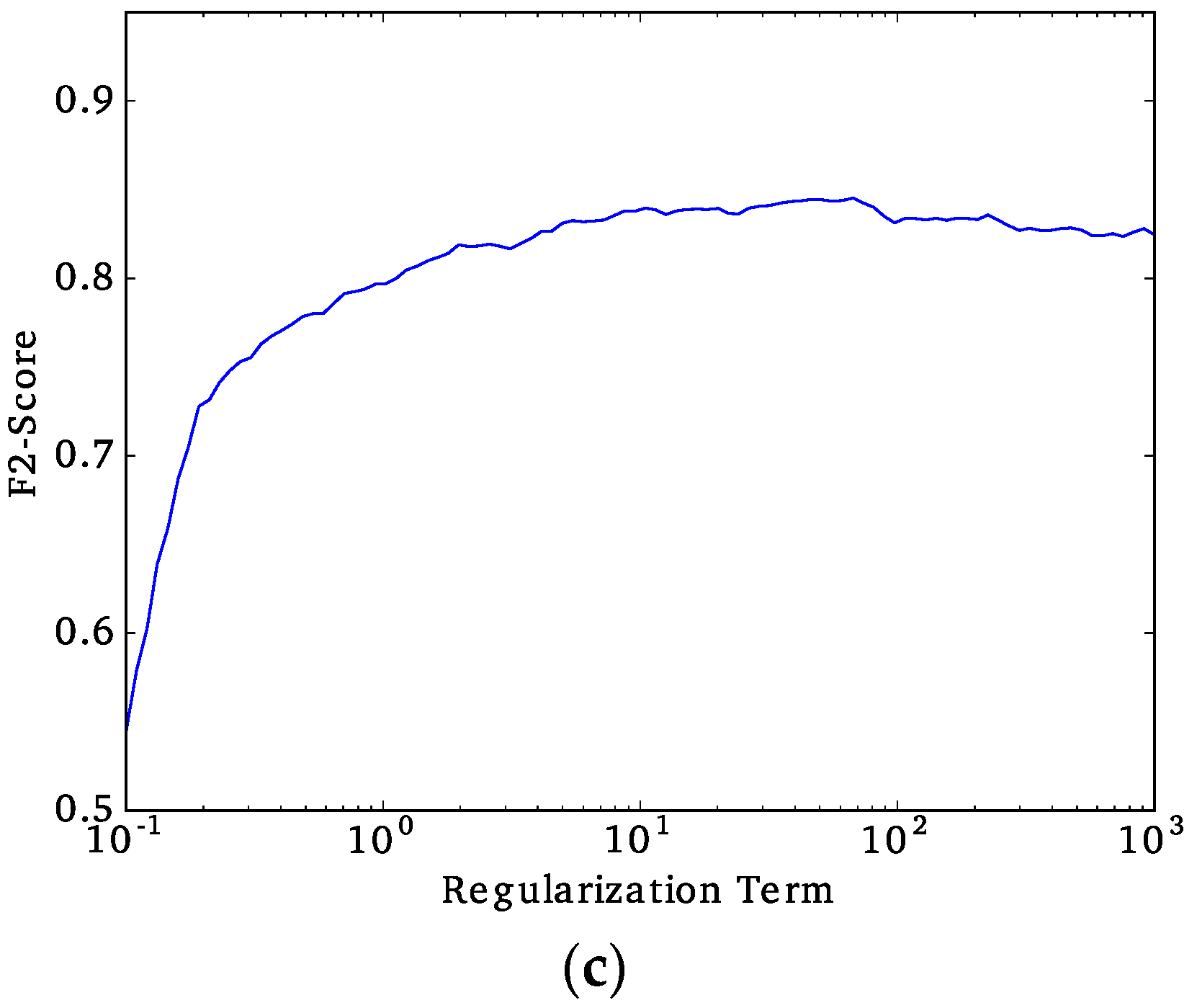
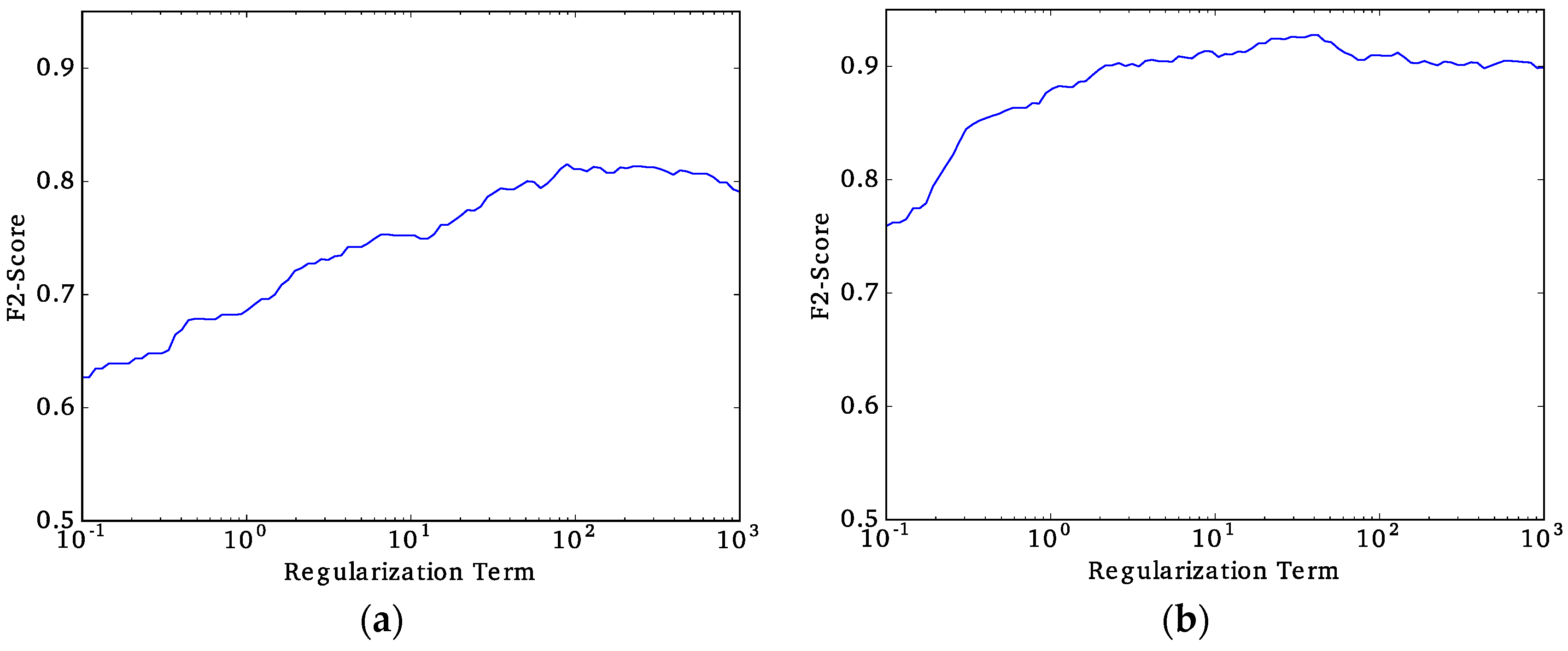
Once we have defined the best performing approach (unified or multi-model) and the best classifier, the next step is to tune the regularization constant to avoid overfitting the data and fine-tune the decision threshold to obtain the final
F2-scores. The regularization constant is exhaustively tuned by evaluating the
F2-score that is obtained while changing the regularization constant. The regularization constant that results in the highest
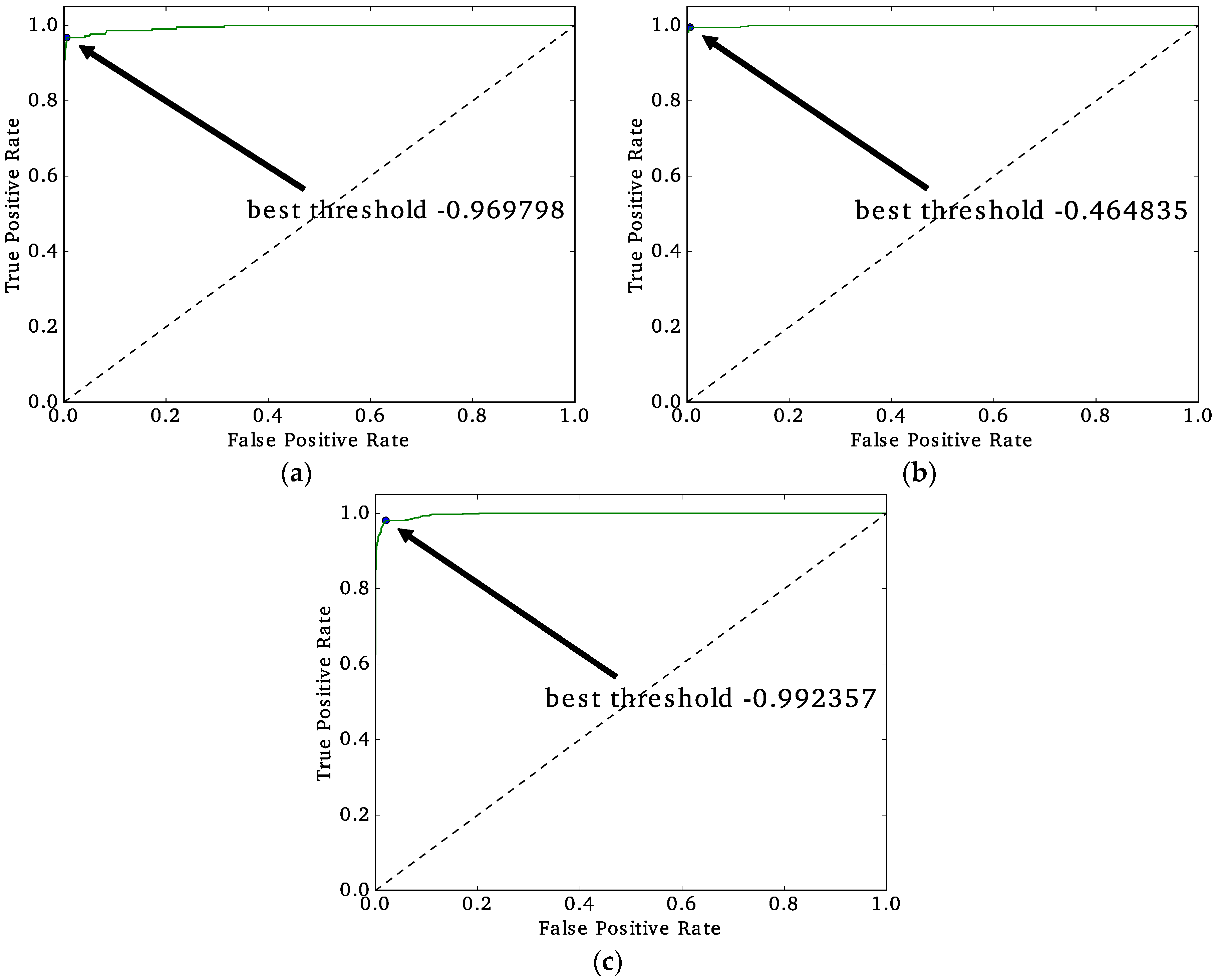
F2-score is defined as the final choice. The decision threshold is the value for which the classifier decides whether a particular observation is classified as slum or no-slum. The decision threshold is selected by using the Receiver Operating Characteristic (ROC) curve, which is a visualization of the False-Positives rates (
X-axis) and True-Positives rates (
Y-axis) while changing the decision thresholds. The machine learning bibliography suggests that the threshold is defined as the closest point to the upper-left corner of the ROC curve. It is important to note that the decision thresholds of the logistic regression reported in
Section 3 are not bounded between 0 and 1, which is equivalent to using the
X-axis for the final decision.
To ensure the tuning process is fair (regularization constant, decision threshold), only observations are used in the training dataset, which is accomplished by using cross-validation F2-scores. To obtain the cross-validation F2-scores, the first step is to divide the training dataset into k equal sized parts. On a single iteration, a classifier (with a specific regularization constant and decision threshold) is trained on k − 1 parts and tested in the remaining part to keep the F2-score. This process is repeated k times to ensure that each part is used once for testing. The final cross-validation F2-score is the average of the obtained F2-score for each iteration. Our parameter selection is based on 10-fold cross-validation.
2.4. Slum Changes in Time
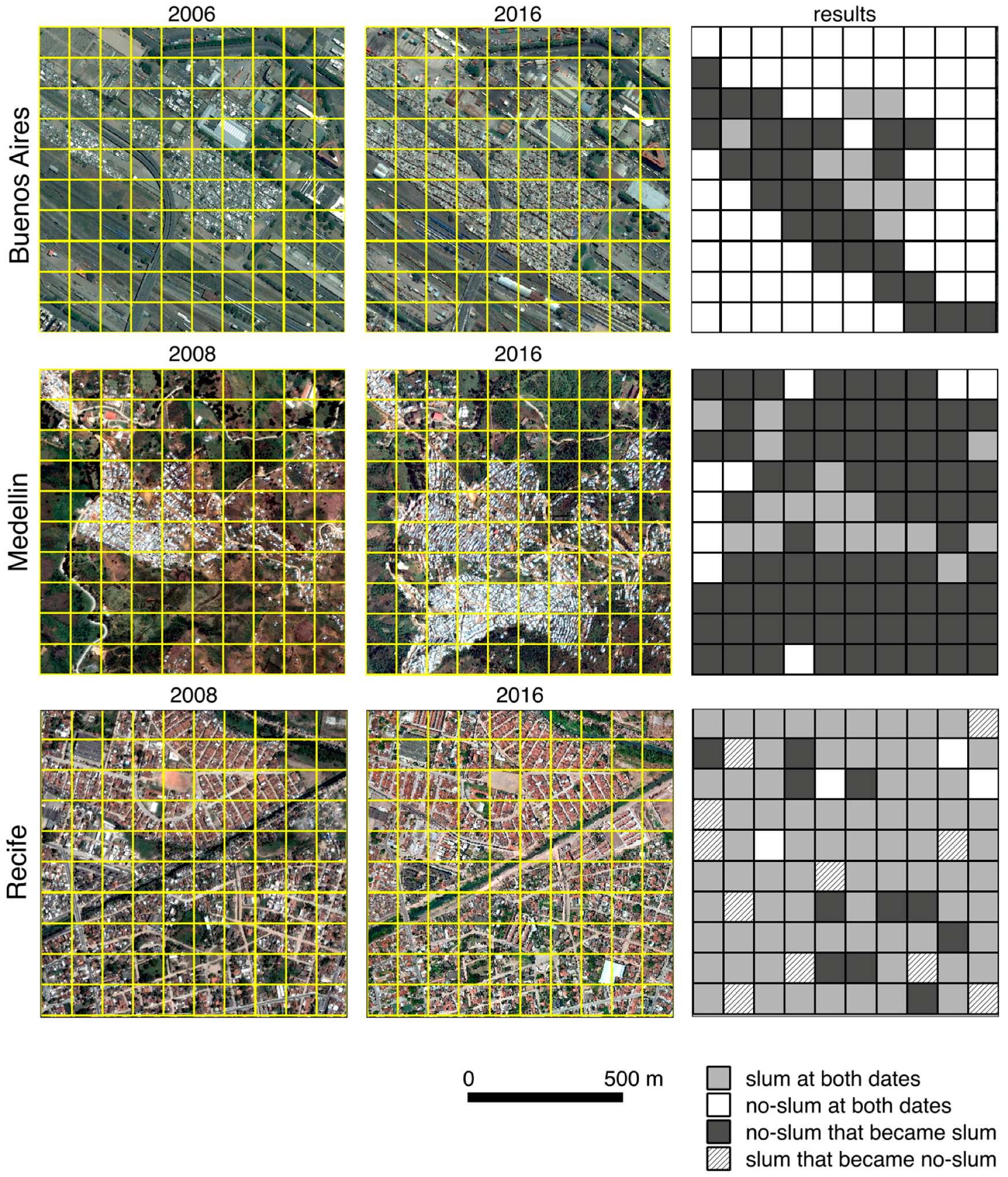
As stated above, we downloaded historical GE images for specific sectors of each city from roughly a decade ago (period t − 1) to perform change analysis. We selected identified slum sectors of 1 km2 in the recent GE images (2016), and downloaded historical images of those sectors, from one decade ago, using historical imagery functionality in Google Earth. We applied relative radiometric normalization between the t − 1 image and the most recent image in each city. This process minimizes the differences in image data due to changes in atmospheric conditions, solar illumination, and view angles between images acquired at different dates. We extracted image features using the same regular grid of square cells and used the classifier model trained with the 2016 image-extracted data (period t) to classify each cell within the sector as either slum or no-slum. Then, cell by cell, we compared the results of the two dates (t vs. t − 1) and assigned different colors to differentiate the areas that were classified as slum for both dates, areas that were classified as no-slum for both dates, areas that were classified as no-slum for the t − 1 date but were classified as slum for the t date, and areas that were classified as slum for the t − 1 date and no-slum for the t date.
Following this rationale, we tested if the proposed approach could be useful to analyze slum dynamics over time by detecting areas that became slum areas, stable areas (no change), and areas that were slum areas and became no-slum areas by upgrading or through urban renovation processes.
4. Conclusions
This study explored implementing a low-cost standardized method for slum detection using spectral, texture and structural features extracted from VHR GE imagery that was utilized as input data and assessed the capability of three ML algorithms to classify urban areas as either slum or no-slum. Using data from Buenos Aires (Argentina), Medellin (Colombia), and Recife (Brazil), we determined that Support Vector Machine with radial basis kernel (SVMrbk) performed the best with a F2-score over 0.81.
In addition, we determined that the specific characteristics of each city are important to consider and preclude the use of a unified classification model. The ML algorithms performed best for Medellin and Recife and resulted in F2-scores of 0.98 and 0.87, respectively. The image-derived features performed better for slum detection in these cities because their slum areas have a different spatial pattern and texture than no-slum areas and exhibit significant variations in the use of building and roofing materials.
The proposed workflow requires more sophistication to properly track changes over time because for the implemented ML algorithms, recall was given a higher priority than precision to obtain a good identification of the more problematic regions within the cities; false positives occurred in the classification results that adversely impact the change analysis between different dates. However, the proposed approach did identify recently and informally occupied urban areas that possessed slum characteristics, where the changes in local heterogeneity and the spatial pattern are clearly identified and were different from occupied formal areas. Changes in the slum status of an area because of upgrading processes would still be difficult to identify because those processes do not significantly change the spatial pattern and texture of the urban areas, which are the aspects quantified by the image-derived variables.
A suggestion for future studies is to use algorithms for object and scene recognition on images that are obtained from Google Street View to generate a new set of features that can improve the performance of our classification models. Street views and satellite imagery for slum identification can also be an important tool for supporting programs such as the Trust Fund for the Improvement of Family Housing that is led by the Development Bank of Latin America and the Foundation in Favor of Social Housing.


