Article

Downscaling Land Surface Temperature in an Arid Area by Using Multiple Remote Sensing Indices with Random Forest Regression

School of Earth Science and Engineering, Hohai University, 8 Buddha City West Road, Nanjing 210098, China
*
Author to whom correspondence should be addressed.
Remote Sens. 2017, 9(8), 789; https://doi.org/10.3390/rs9080789
Submission received: 12 May 2017 / Revised: 23 July 2017 / Accepted: 29 July 2017 / Published: 31 July 2017

Abstract

:
Many downscaling algorithms have been proposed to address the issue of coarse-resolution land surface temperature (LST) derived from available satellite-borne sensors. However, few studies have focused on improving LST downscaling in arid regions (especially in deserts) because of inaccurate remote sensing LST products. In this study, LST was downscaled by a random forest model between LST and multiple remote sensing indices (such as soil-adjusted vegetation index, normalized multi-band drought index, modified normalized difference water index, and normalized difference building index) in an arid region with an oasis–desert ecotone. The proposed downscaling approach, which involves the selection of remote sensing indices, was evaluated using LST derived from the MODIS LST product of Zhangye City in Heihe Basin. The spatial resolution of MODIS LST was downscaled from 1 km to 500 m. Results of visual and quantitative analyses show that the distribution of downscaled LST matched that of the oasis and desert ecosystem. The lowest (approximately 22 °C) and highest temperatures (higher than 37 °C) were detected in the middle oasis and desert regions, respectively. Furthermore, the proposed approach achieves relatively satisfactory downscaling results, with coefficient of determination and root mean square error of 0.84 and 2.42 °C, respectively. The proposed approach shows higher accuracy and minimization of the MODIS LST in the desert region compared with other methods. Optimal availability occurs in the vegetated region during summer and autumn. In addition, the approach is also efficient and reliable for LST downscaling of Landsat images. Future tasks include reliable LST downscaling in challenging regions.

Graphical Abstract

1. Introduction

Land surface temperature (LST) dominates in biophysical–chemical processes at the land–atmosphere interface. LST has been widely used in evapotranspiration estimation, urban heat island characterization, and drought monitoring [1,2,3,4,5,6,7]. Thermal infrared remote sensing (TIRS) in high temporal or spatial resolution can be used to estimate LST dynamically and macroscopically [8,9,10,11,12]. MODIS LST product is widely used in moderate–low spatial resolution. Thus, it can provide daily information but is limited to low-spatial resolution. Therefore, downscaling of MODIS LST must be investigated to enhance the spatial resolution of thermal images with relatively low resolution [13].
LST downscaling is known as TIRS image sharpening, disaggregation, or scale decomposition [14,15]. Downscaling models can be classified into statistical regression and physical mechanism-based models [15,16,17,18,19,20,21,22,23,24,25], such as modulation-based methods. Modulation-based downscaling achieves excellent downscaling effect because of LST function or thermal radiation brightness and land cover types based on thermal radiation and spectral mixture analysis [26,27]. The statistical regression model is commonly used because of its ease of operation and acceptable downscaling accuracy. Statistical regressions connect LST with remote sensing indices, which are extracted from high-resolution, visible, near-infrared, or short-wavelength infrared bands through statistical correlations. Several vegetation indices are widely used to downscale LST effectively especially in vegetated regions; these indices include normalized difference vegetation index [20], fractal vegetation index [21,22,23], vegetation dryness index [28,29,30], and soil-adjusted vegetation index (SAVI) [26]. Various types of remote sensing indices are used in statistical regressions in other types of land surfaces; these factors include normalized difference building index (NDBI) [27] in building areas and normalized difference dust index (NDDI) [31] in bail soil areas.
The most common statistics-based downscaling algorithms are linear regression models, including disaggregation procedure for radiometric surface temperature (DisTrad) method [20], thermal sharpening (TsHARP) algorithm [21,22,23], pixel block intensity modulation (PBIM) algorithm [32], emissivity modulation (EM) algorithm [33], and high-resolution urban thermal sharpener(HUTS) algorithm [34]. However, linear regression formula is occasionally incapable of representing nonlinear relationships between LST and remote sensing indices. Thus, various models were established to present linear or nonlinear relationships between LST and factors, including piecewise linear and nonlinear regression model [35,36], conditional expectation model [37], co-Kriging model [38,39], Bayesian-based model [40], artificial neural networks [41], genetic algorithm techniques [42], support vector machines [43], and random forest (RF) regression [44]. Notably, Hutengs and Vohland [44] pioneered RF regression with red and near-infrared (NIR) bands, which are related to vegetation index to downscale MODIS LST products in the vegetated regions; this method yielded accurate results. However, downscaled results were probably unsatisfactory in arid non-vegetated regions because of severe underestimation of MODIS LST products over the area [45].
Therefore, our study proposes a multi-scale-factor downscaling method based on RF regression and multiple remote sensing indices to solve the problem of MODIS LST products in arid regions. A detailed analysis of errors with spatial autocorrelation between the original LST image and downscaled products is presented. The downscaled images are compared with images obtained using other downscaling methods through visual and quantitative analyses. The rest of this paper is organized as follows. Section 2 presents information regarding the study area, data gathered, and proposed method. Section 3 evaluates the downscaling results. Section 4 discusses the findings. Section 5 concludes the paper.

2. Material and Methods

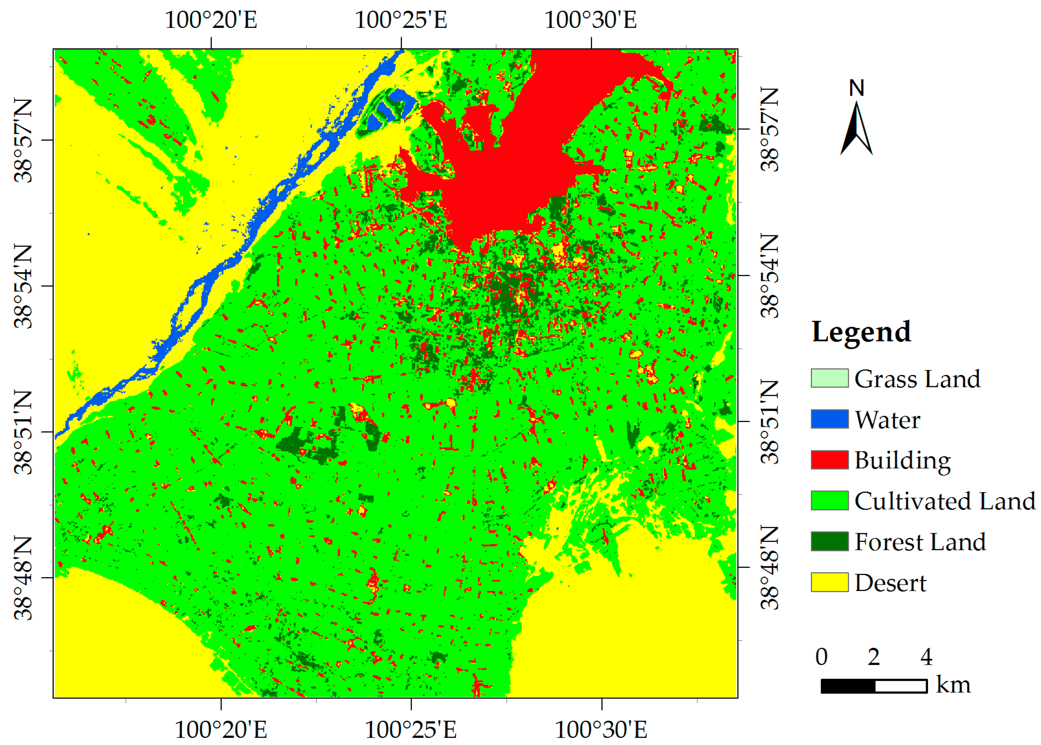
2.1. Study Area and Data Description

The Heihe Basin (97°24′–102°10′E, 37°41′–42°42′N), with an area of 130,000 km2, is the second largest inland river basin in Northwest China. Our study area is situated in an oasis–desert ecotone of Zhangye City (31°14′–32°37′N, 118°22–119°14′E) within the middle reaches of the Heihe Basin. The area experiences an arid continental climate and long dry season (from October to May) and short rainy season (from June to September). The annual mean temperature in the area is 6.5 °C and the average annual precipitation (evaporation) is 115.6 (2107.1) mm [46]. June to September are the hottest and most humid months, in which the average maximum air temperature reaches 39.3 °C The study area contains four main land cover types, namely, wetland, impervious surfaces, vegetation, and desert, which are located in the northernmost, north, middle, and northwest (southeast and southwest) parts, respectively. The oasis locates in the middle of this region surrounded by the desert. Six ground sites (wetland, maize, orchard, Gobi, wilderness, and desert sites) were selected from large flat areas of the four land cover types (Figure 1).
All selected sites are parts of the Heihe Watershed Allied Telemetry Experimental Research (HiWATER), which is an ongoing watershed-scale eco-hydrological experiment designed from an interdisciplinary perspective to address problems including heterogeneity, scaling, uncertainty, and closing of the water cycle at the watershed scale [47].
All ground observation data were provided by the Cold and Arid Regions Science Data Center at Lanzhou [48]. The actual LST was estimated from upwelling and downwelling longwave radiation observed by pyranometers using the following equation:
T s = [ R l u ( 1 ε ) R l d ε σ ] 0.25
where Rlu (Rld) is the surface upwelling (downwelling) longwave radiation, ε is land surface emissivity (LSE), Ts is LST, and σ is the Stefan–Boltzmann constant. The temporal resolution of all ground observation is 10 min. Furthermore, the ground observation data during satellite overpassing were chosen to validate the retrievals (Table 1).
The MODIS products were acquired at 5:55 (UTC) on 3 September 2012 (autumn) and used in this study. The products were available in Level 1 and Atmosphere Archive and Distribution System. The MOD11 datasets provide the LSE (bands 31 and 32) and LST with 1-km spatial resolution, and the MOD09 datasets provide the reflectance of bands 1–7 with 500-m spatial resolution [49]; these datasets are used to acquire remote sensing indices to downscale the resolution of MOD11 LST from 1 km to 500 m. The images under a clear sky were acquired on 17 April 2013, 15 June 2012, and 22 February 2013 to reveal the availability of our approach in other seasons (spring, summer, and winter), except for the image in the autumn.
The Advanced Spaceborne Thermal Emission and Reflection Radiometer (ASTER) LST and LSE datasets on 3 September 2012 in the middle reaches of the Heihe Basin were selected. The ASTER LST in the arid region exhibits higher spatial resolution (90 m) and is more accurate than that of MODIS because of the satisfactory estimation of ASTER LSE [48,50]. The ASTER LST was provided by the Cold and Arid Regions Science Data Center at Lanzhou. A validation reference is not available for LST simulation; as such, the ASTER images were upscaled to 500-m resolution to ensure that simulation could be validated by ASTER LST.
In addition, the land use/land cover (LULC) dataset was provided by the Cold and Arid Regions Science Data Center at Lanzhou with an overall accuracy of 92.19% [51,52]. The spatial and temporal resolutions are 30 m and 1 month, respectively (Figure 2).
The Landsat 8 Operational Land Imager (OLI) and TIRS image were acquired on 21 July 2013 and then used in this study to evaluate the applicability of our approach for the satellite images in middle-high resolution. The Landsat 8 datasets, which were provided by the United States Geological Survey, included OLI and TIRS images with 30- and 100-m spatial resolutions, respectively. LST and remote sensing indices were calculated using these images.

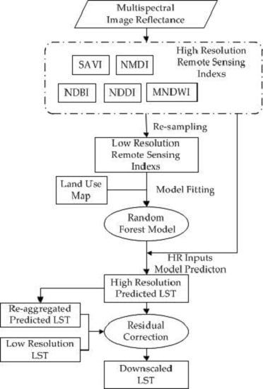
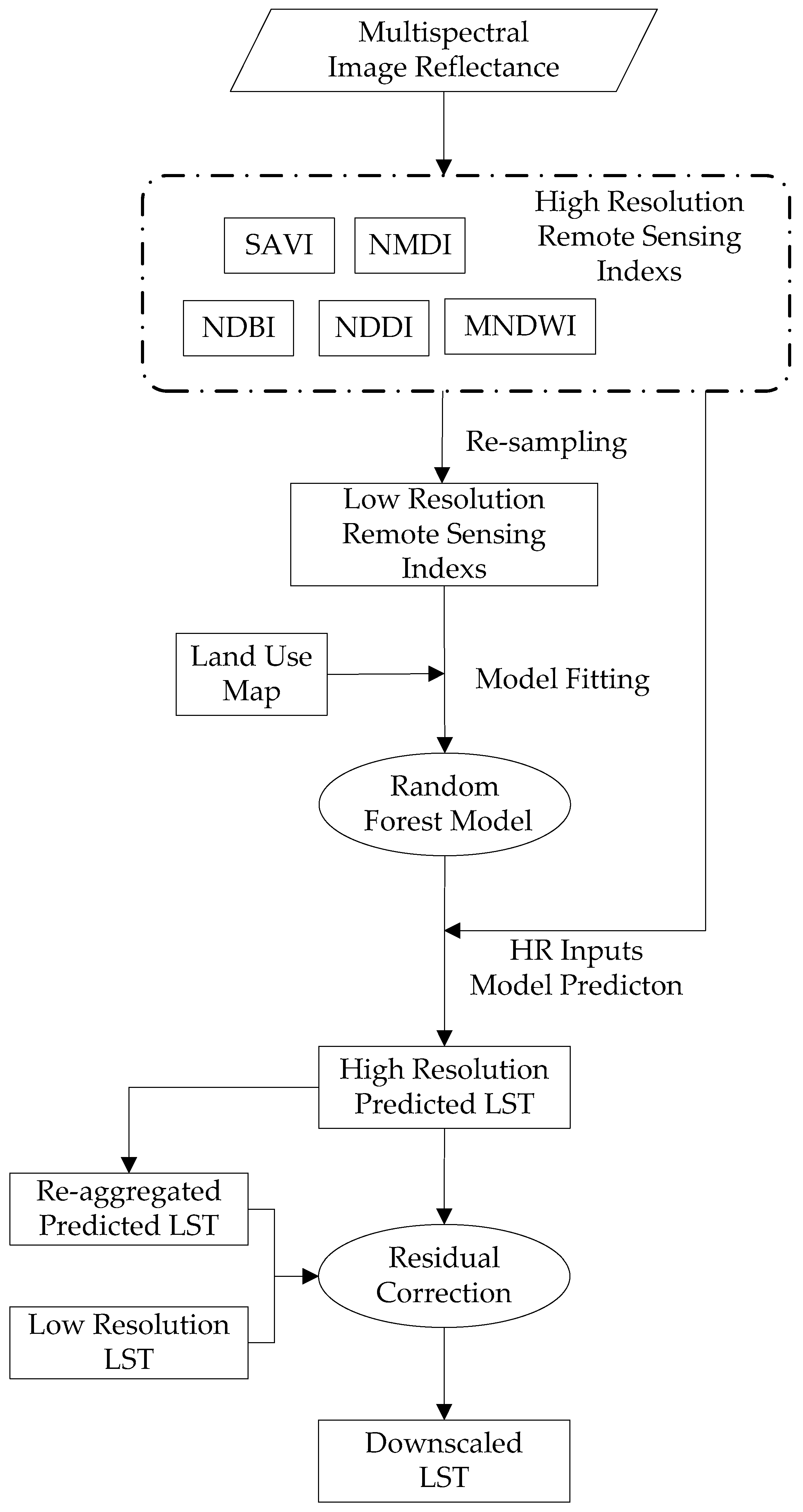
2.2. Downscaling Methods

MODIS LST products are characterized with coarse spatial resolutions. Regression models between ancillary environmental predictors and LST have been established to enhance LST resolution. If the relationships between LST and predictors do not change with spatial resolution, then a detailed high-resolution LST can be estimated by predictors using such relationships.
RF is a nonlinear statistical ensemble bagging method. RF employs recursive partitioning to divide data into many homogeneous subsets, called regression trees, and averages the results of all trees. Each tree is independently grown to its maximum size based on a bootstrap sample from the training dataset without any pruning. In each tree, the ensemble predicts data that are not in the tree (the out-of-bag: OOB data). By calculating the difference in the mean square errors between the OOB data and data used to grow the regression trees, the RF algorithm provides an error of prediction called the OOB error of estimate for each variable. The binary splits are selected by minimizing the sum-of-squares error between the response variable and the predicted response caused by a specific split.
The choice of appropriate predictor variables in RF downscaling approach should refer to existing correlations between LST and many biophysical variables. In previous research on LST downscaling with RF, the reflectance of NIR and red wavebands was selected as predictors. However, these wavebands are not sensitive to recognizing the characteristics of some types of land cover, especially for desert that dominates a large part of the arid region. Therefore, in this paper, some remote sensing indices related to land status (such as vegetation cover, soil moisture, water cover, impervious surface cover, and desert) were selected; these factors include SAVI [53], normalized multi-band drought index (NMDI) [53], modified normalized difference water index (MNDWI) [26], NDBI [27], and NDDI [31]. NMDI was selected to evaluate vegetation stress by soil water.
RF regression trees model the relationship between multiple remote sensing indices and LST simulation by a set of decision rules. The LULC was not regarded as the predictor to facilitate the recognition of the influence of LULC on the LST downscaling in the future. Accordingly, a model was established for each land cover. Therefore, for each land-cover type, model training on coarse LSTc and input variables is obtained as follows:
LST F = f ( SAVI C , NMDI C , MNDWI C , NDBI C , NDDI C )
where the subscript C indicates the variable in the coarse resolution and the subscript F refers to the variable fitted by those variables.
The residual temperature (e) was the difference between the original LST (LSTO) and the LSTF, as shown in Equation (2). This difference is the model estimation error:
e = LST F LST O
Therefore, from the coarse-resolution LST, the simulated LST with coarse resolution (LSTC) could be estimated as follows:
LST C = f ( SAVI C , NMDI C , MNDWI C , NDBI C , NDDI C ) + e
Given the scale invariance, the trained model was applied to the five remote sensing indices with high resolution. Subsequently, a simulated, high-resolution LST (LSTH) is obtained, which is given as follows:
LST H = f ( SAVI H , NMDI H , MNDWI H , NDBI H , NDDI H ) + e
where H indicates the high-resolution variable. For convenience, LSTH (LSTC) is regarded as the downscaled (simulated) LST, and LSTO is regarded as the original LST.
In the region with every kind of land cover, Equation (5) holds. Accordingly, the 1-km LST is downscaled by these regression models in each land cover. For convenience, the proposed approach was called multiple remote sensing indices approach of random forest (MIRF). In our study, a 1-km coarse resolution is the spatial resolution of MOD11 LST, while a 500-m resolution is the spatial resolution of remote sensing indices. A detailed procedure is presented in Figure 3.
Two typical LST downscaling approaches were selected, namely, DisTrad and basic RF, to evaluate the effectiveness of our approach. The DisTrad approach downscaled LST using a least-squares fit of LST and vegetation index [20]. Vegetation index in a high spatial resolution is selected as a predictor to downscale the LST in low spatial resolution. The basic RF approach was based on RF and two predictors (red band and NIR reflectances) [44]. Unlike MIRF, the land cover data were also another predictor to simulate LST. The relationship of LST and all three predictors in high spatial resolution are regressed by RF to downscale the LST in low spatial resolution.
In addition, the applicability of the proposed method for satellite images in middle-high spatial resolution has been evaluated by Landsat and MIRF approach. The Landsat OLI images were initially adjusted with the Fast Line-of-sight Atmospheric Analysis of Hypercubes atmospheric correction algorithm [54]. Then, the LST was retrieved using single-channel method, OLI, and TIRS datasets [55]. For convenience, the TIRS images with 100-m resolution were resampled into 90-m images by the nearest neighbor method, whereas the OLI images with 30-m resolution were resampled into 90-m images by aggregation. The 30-m OLI images were high-resolution images, whereas the 90-m OLI and TIRS images were coarse-resolution images in the MIRF approach.

2.3. Evaluation Measures

Three measures, namely, coefficient of determination (R2), bias, and root-mean-square error (RMSE) [32,56], were used to evaluate the downscaling effect of the MIRF algorithm and compare the proposed algorithm with three other downscaling methods.
In the equation below, R2 is the coefficient of determination between the original and downscaled images. A high R2 indicates a satisfactory downscaling. This coefficient is given by the following:
R 2 = 1 ( LST S LST R ) 2 ( LST S LST R ¯ ) 2
where LSTS is the simulated LST (Equations (4) and (5)), LSTR is the reference LST, and LST R ¯ is the average of LSTR in the entire image. In detail, the LSTR is the LST observed by the ground instrument in the direct validation, whereas the LSTR is the LST obtained by ASTER in the cross validation.
Bias and RMSE were used to test the errors between the original LST image and the downscaled image. The calculation formulas for bias and RMSE are as follows:
b i a s = i = 1 n ( LST S LST R ) n
RMSE = 1 n i = 1 n ( LST S LST R ) 2
where n represents the number of pixels of the image.

3. Results

3.1. Downscaling Results

3.1.1. Spatial Distribution of LST and Remote Sensing Indices

The five remote sensing indices, SAVI, NMDI, MNDWI, NDBI, and NDDI, were extracted from the MOD09 products (Figure 4). Comparison results of Figure 2 and Figure 4 show that the spatial distributions of the five remote sensing indices were consistent with those of four land-cover types (i.e., vegetation, desert, water, and impervious surface). Thus, these remote sensing indices can accurately characterize the four land-cover types.
The oasis, located in the middle of the study area, exhibited SAVI and NMDI higher than 0.5 and 0.25, respectively, indicating a vegetated area with relatively moist soil. In the southeastern desert, southwestern wilderness, and northwestern Gobi, an area with NDDI higher than 0.35 was located with no vegetation and sand. The medium remote sensing indices were located in the urban area of the northern region. Furthermore, mixed-land covers occupied the other pixels of the study area.
The LST distribution (500-m resampled ASTER LST) is presented in Figure 5a. The average temperature in the study area was 30 °C The lowest temperature (approximately 22 °C was detected in the middle oasis region with luxuriant vegetation, which exhibited high SAVI; by contrast, the highest temperature (higher than 37 °C was located in the desert region with high NDDI. Medium temperatures (approximately 32 °C were also recorded in the urban region, which had medium remote sensing indices. Therefore, the LST distribution was evidently related to remote sensing indices. In our study, LST and LULC relationship was also similar to that in other arid regions [57,58].
Figure 5b shows the 1-km MOD11 LST; its distribution is similar to that of the 500-m resampled ASTER LST. However, LST is coarse at 1Km resolution, particularly for oasis areas. Thus, the downscale is necessary to sharpen the LST resolution.
The temperature distribution correlated with the remote sensing indices, in depicting the distribution of the oasis and desert ecosystem. The lowest temperature corresponded to the high SAVI in the oasis region, whereas the highest temperature corresponded to the high NDDI in the desert region. Medium temperature was related to the medium remote sensing indices in the urban area of the northern region.

3.1.2. Downscaling Performance

Figure 5c shows the LST downscaling performance of our approach. The average downscaled temperature in the study area was 29 °C Comparison of Figure 5b with Figure 5c shows that the proposed downscaling method improved the spatial resolution of the original LST image, especially in the middle region in which low LSTs are indicated in blue, corresponding to the oasis areas. Our simulated LST image could identify detailed information in the northwestern region corresponding to the Gobi areas. The LST distribution in Figure 5c is similar to those in the 1-km image of the MOD11 product (Figure 5b), with the lowest, relatively low, and highest temperatures detected in the vegetation, building areas, and desert, respectively. Therefore, our 500-m downscaled LST showed spatial reliability and provided more detailed information than the 1-km LST of MOD11 product in Figure 5b.

3.2. Evaluation of Downscaling Results

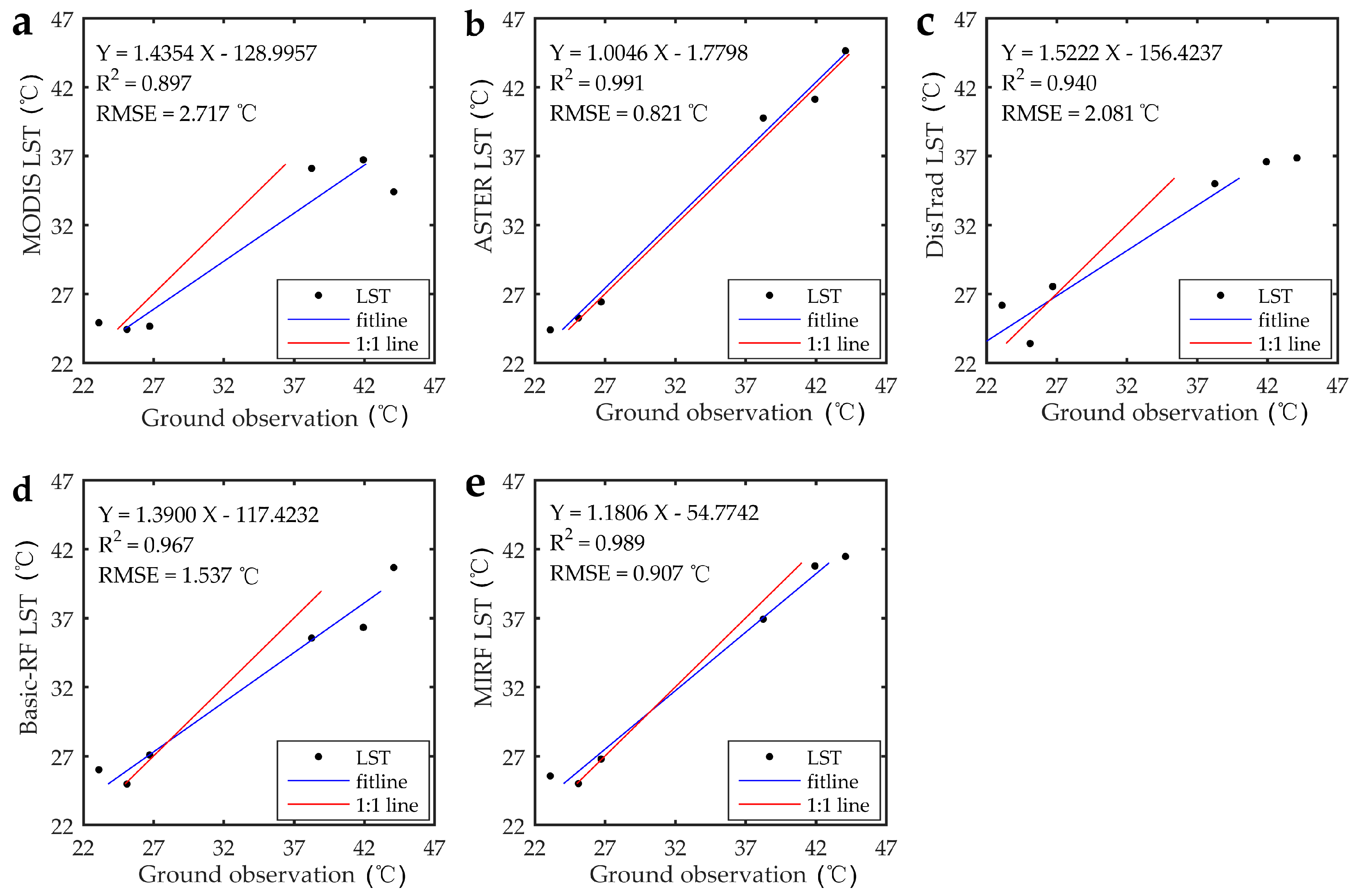
3.2.1. Direct Validation

Figure 6 shows the relationship between LST ground observation (donated by x-axis) and downscaled LST (donated by y-axis) at the time of satellite overpass. In general, relative to the observation with 10 min of temporal scale, the downscaled LST of our approach was generally accurate and underestimated, with bias, RMSE, slope, and R2 values of 0.46 °C, 0.91 °C, 1.18, and 0.99, respectively. The accuracy of downscaled LST using our approach was higher than the accuracy of MOD11 LST (RMSE of 2.72 °C (Figure 6a. In addition, the accuracy of our approach was also better than that of other downscaling approaches in previous literature (RMSE of approximately 2 °C [20,44].
Table 2 also shows the comparison between ground observation and downscaled LST using our approach in all six sites. The downscaled LST was generally underestimated and in relatively good agreement with ground observations at most sites, with bias of −2.64 to 2.45 °C The highest accuracy was obtained at orchard and maize sites, with bias values of 0.06 °C and −0.11 °C respectively. The downscaled LST in wetland and desert sites was less satisfactory, with bias of 2.45 °C and −2.64 °C respectively. The underestimation in the desert site is possibly related to MOD11 LSE product errors. In comparison with the severe underestimation of MOD11 LST (−9.71 to −2.16 °C at the sites in the desert region (i.e., Gobi, desert, and wilderness sites), the proposed approach obviously improves the accuracy of LST at these sites. The validation revealed the viability of the proposed approach.

3.2.2. Cross Validation

Figure 6b and Table 2 showed the accuracy of ASTER LST with errors of −0.82 to 1.50 °C at the six sites. Therefore, the downscaled LST was validated by ASTER LST to reveal the spatial distribution of the downscaled LST error. In comparison with the resampled 500-m ASTER LST, the 500-m downscaled LST had pixel-average R2 and RMSE values of 0.84 and 2.4 °C for the entire image, respectively (Figure 7d). The pixels with LST errors of −1.0 to 1.0 °C, −3.0 to −1.0 °C, 1.0 to 3.0 °C lower than −3.0 °C and higher than 3.0 °C accounted for 43%, 19%, 16%, 18%, and 4% of all the pixels, respectively (Figure 8). In half of the pixels, the discrepancies between the retrieved and simulated LSTs were less than 1 °C and within the scope of the retrieved accuracy [52]. Thus, reliable downscaling results were obtained in most parts of the area.
As shown in Figure 7, a systemic underestimation occurred in the desert region with temperature higher than 37 °C specifically in southeastern desert. This phenomenon may have been induced by MOD11 LST underestimation. In addition, few pixels with LST overestimation were found in the northwestern boundary region between the oasis and desert, where Heihe River was located. This outcome could be due the mixed pixel of the narrow river [59]. Thus, we also analyzed accuracy depending on the different types of surfaces to reveal the overall accuracy of the downscaling result. The RMSE results in water, vegetation, impervious surface, and bail soil regions were 2.79, 0.40, 2.50, and 3.34 °C respectively. Thus, our results demonstrate a higher accuracy in the oasis region than in other areas. This observation was similar to the results of other studies that revealed satisfactory accuracy in the vegetated region with RMSE of less than 1 °C [9]. This observation can be attributed to the close relationship between vegetation indices and LST.

3.3. Comparison of Approaches

As shown in Figure 7, all downscaling methods improved the spatial resolution of the original LST image (Figure 5b). Some detailed information within the same land cover was found in the downscaled images (Figure 7b–d); in comparison, the same information was not found in the original image (Figure 5b). The downscaled LST images maintained the thermal and spatial distribution characteristics of the original LST image. Relative to the 500-m ASTER LST, regardless of the water area, the downscaling result of DisTrad and basic RF approaches had R2 (RMSE) values of 0.58 (3.87 °C and 0.81 (2.60 °C, respectively, whereas the value obtained using the proposed approach was 0.84 (2.42 °C. Similarly, compared with the ground observation at all six sites, the R2 (RMSE) values of DisTrad, basic RF, and the proposed approach are 0.94, 0.97, and 0.99 (2.08, 1.54, and 0.91 °C, respectively (Figure 6). All approaches decrease the error of MOD11 LST (2.72 °C, but the accuracy of the proposed approach is higher than that of the two mentioned approaches.
In detail, most errors of the three methods ranged from −1 to 1 °C Most of the errors were less than 1 °C for the MIRF algorithm, and errors lower than −3 °C were found for the DisTrad and basic RF approaches (Figure 8). The accuracy of the proposed approach exceeded those of the DisTrad and basic RF approaches in the vegetation, impervious surface, and desert regions. The proposed approach can downscale LST in the water area, whereas the DisTrad approach is not capable of downscaling in that area.

3.4. Applicability of Approach

3.4.1. Applicability in Different Seasons

Just like the situation in the autumn which is shown in Figure 5c, the downscaling results of the MIRF algorithm in the other three seasons are shown in Figure 9. Obviously, the downscaling results of MIRF were more accurate than those of the MOD11 LST in all seasons (Table 2 and Table 3). Compared with the ground observation, the 500-m downscaled LST has an error of −4.41 to 3.69, −2.32 to 4.80, and 0.16 to 5.27 °C at six sites in the summer, winter, and spring, respectively. Considering an error of −2.64 to 2.45 °C in the autumn, our approach shows better applicability in the autumn than in the other three seasons.
In detail, the downscaling result of our approach at the vegetated sites (maize and orchard sites) has a better accuracy than that of other sites in summer and autumn. In spring and winter, the accuracy in vegetated sites decreased, which may be related to the spare vegetation in the oasis after harvest. Accordingly, the lowest LST occurred in the oasis in summer and autumn, while a medium LST was observed in oasis in spring and winter (Figure 9).
Generally, the MIRF algorithm can be applied in all seasons, especially in summer and autumn. Furthermore, the best availability occurred in vegetated regions in these two seasons.

3.4.2. Applicability for Satellite Images in Middle-High Resolution

Figure 10 shows the LST distribution retrieved by Landsat8 images (90-m spatial resolution) and downscaled by Landsat OLI datasets (30-m spatial resolution). More detailed LST information appeared after downscaling, especially in the building region (green rectangular block) and the southeastern desert (red rectangular block). The pixel average temperature in the study area was 32.88 °C for Landsat LST and 34.84 °C for the downscaling result. The discrepancy between Landsat LST and the downscaling result was also approximately 2 °C for each land-cover area.
The downscaled LST error ranged from 0.16 to 4.53 °C at all sites compared with the ground observations, with original Landsat LST error scores of −2.63 °C to 3.86 °C (Table 4). As expected for the Gobi site, the LST error decreased after downscaling at other sites, especially at vegetated sites (wetland and maize sites). Compared with the Landsat LST, the downscaling error result decreased from more than −2 °C to near 0 °C at these two sites. Therefore, similar to its applicability in the MODIS images, our approach shows its applicability in the Landsat images, which is one of most representative satellite images with middle-high resolution.

4. Discussion

The MIRF algorithm is credited for its nonlinear expression, multiple remote sensing indices, and satisfactory accuracy. First, the MIRF algorithm, which is characterized by nonlinear regression, minimizes the risk of overfitting and provides accurate downscaling because of the RF approach. Unlike other linear regression approaches for LST downscaling (e.g., DisTrad), the proposed nonlinear regression utilizes multiple remote sensing indices selected according to the land cover. Second, compared with other approaches with single vegetation indices (e.g., DisTrad and basic RF), multiple relevant remote sensing indices can characterize LULC precisely, especially in non-vegetated areas. Accordingly, the input of multiple remote sensing indices also improves downscaling in the desert region. Third, compared with the original MODIS LST product and the downscaling result of DisTrad and basic RF, the MIRF algorithm achieves a satisfactory downscaling effect, especially in the Gobi or desert sites. Therefore, our approach improves both the spatial resolution and accuracy of MODIS LST product, especially in arid non-vegetated regions.
However, our algorithm has some limitations in LST downscaling. First, the relatively large error observed at the wetland site is probably attributed to the inappropriate expression of the MIRF algorithm in the vegetated region. For the selected LULC, wetland was classified as the vegetation in this region. Unlike crop land, wetland was mixed with water and vegetation. Considering that the crop land dominated the vegetated area, the regression in vegetated area is more available to downscaling in the crop land. Therefore, the effectiveness of the regression in the wetland was limited. More detailed LULC benefits the regression. Therefore, the accuracy of the land cover product is crucial to the effectiveness of the MIRF algorithm, especially in mixed area. Caution should be exercised when the study area is mixed and the land cover product is unreliable. Second, the proposed algorithm is used in LST downscaling for polar satellites (e.g., MODIS and Landsat). However, the effectiveness of the MIRF algorithm is limited by the low temporal resolution of the downscaled LST images and the influence of the clouds [60,61]. Thus, the LST downscaling of geostationary meteorological satellite images in low-spatial and high-temporal resolutions is necessary to continuously estimate LST intra-daily dramatic variation [32,53].

5. Conclusions

This paper presents a strategy for downscaling LST in an arid region using multiple remote sensing indices according to the RF method. The comparison results based on statistical measures and visual analyses show that MIRF achieves satisfactory downscaling performance. The distribution of downscaled LST matches that of the oasis and desert ecosystems. Relative to the ground observation, the downscaled LST was generally accurate and underestimated with bias, RMSE, and R2 values of 0.46 °C 0.91 °C and 0.99, respectively. The R2 and RMSE values between the 500-m downscaled result and the 500 resampled ASTER LST are 0.84 and 2.42 °C respectively. The differences between the ASTER LST and downscaled LST are less than 1 °C in approximately half of the study area, except for the underestimation in the southeastern desert. Spatially, compared with the 500-m resampled ASTER LST, the 500-m downscaled result simply sharpened LST resolution; furthermore, the LST distribution matched the distribution of oasis and desert.
Compared with other algorithms that provide high downscaling accuracy, MIRF has relatively credible downscaling performance, multiple remote sensing indices, and minimization of the MODIS LST product error in the desert region. Furthermore, the optimal availability occurred in the vegetated region during summer and autumn. MIRF can also be applied to moderate- or high-resolution remote sensing images, such as Landsat images, except for application in moderate- or low-resolution remote sensing images. Thus, MIRF exhibits potential in generating useful LST information in the arid region with improved spatial resolution.

Acknowledgments

This study is supported by the National Nature Science Foundation of China (41271538), by the China Postdoctoral Science Foundation Funded Project (2017M611665), by the Fundamental Research Funds for the Central Universities of China, by the Key Project of Water Resources Department of Jiangxi Province (KT201506), by the project funded by the priority academic program development of Jiangsu higher education institution, and by Postgraduate Research & Practice Innovation Program of Jiangsu Province (KYCX17_0503). We thank the Cold and Arid Regions Science Data Center at Lanzhou for providing observation data (http://westdc.westgis.ac.cn) and the LAADS for providing MOIDS products (http://ladsweb.nascom.nasa.gov). We thank professor L.S.M. and X.Z.W. (Beijing Normal University) for their kind assistance in providing field data and help in field visit. We also thank the anonymous referees for their insightful comments and suggestions.

Author Contributions

Yingbao Yang proposed the main idea, offered invaluable suggestions for data analysis, and revised the manuscript thoroughly. Chen Cao performed the experiments and made careful data analysis. Xin Pan designed the experiments and wrote this paper. Xiaolong Li also conceived the experiments and contributed analysis tools. Xi Zhu made some comments on the manuscript.

Conflicts of Interest

The authors declare no conflict of interest.

References

  1. Qin, Z.; Berliner, P.; Karnieli, A. Micrometeorological modeling to understand the thermal anomaly in the sand dunes across the Israel–Egypt border. J. Arid Environ. 2002, 51, 281–318. [Google Scholar] [CrossRef]
  2. Merlin, O.; Duchemin, B.; Hagolle, O.; Jacob, F.; Coudert, B.; Chehbouni, G.; Dedieu, G.; Garatuza, J.; Kerr, Y. Disaggregation of MODIS surface temperature over an agricultural area using a time series of Formosat-2 images. Remote Sens. Environ. 2010, 114, 2500–2512. [Google Scholar] [CrossRef] [Green Version]
  3. Sandholt, I.; Rasmussen, K.; Andersen, J. A simple interpretation of the surface temperature/vegetation index space for assessment of surface moisture status. Remote Sens. Environ. 2002, 79, 213–224. [Google Scholar] [CrossRef]
  4. Eckmann, T.; Roberts, D.; Still, C. Using multiple endmember spectral mixture analysis to retrieve subpixel fire properties from MODIS. Remote Sens. Environ. 2008, 112, 3773–3783. [Google Scholar] [CrossRef]
  5. Voogt, J.A.; Oke, T.R. Thermal remote sensing of urban climates. Remote Sens. Environ. 2003, 86, 370–384. [Google Scholar] [CrossRef]
  6. Zhou, J.; Chen, Y.H.; Wang, J.F.; Zhan, W.F. Maximum Nighttime Urban Heat Island (UHI) Intensity Simulation by Integrating Remotely Sensed Data and Meteorological Observations. IEEE J. Sel. Top. Appl. Earth Obs. Remote Sens. 2011, 4, 138–146. [Google Scholar] [CrossRef]
  7. Su, W.; Yang, G.; Chen, S.; Yang, Y. Measuring the pattern of high temperature areas in urban greenery of Nanjing City, China. Int. J. Environ. Res. Public Health 2012, 9, 2922–2935. [Google Scholar] [CrossRef] [PubMed]
  8. Yang, Y.; Yu, S.; Li, Y.; Lu, D. Integration of multidimensional parameters of polarimetric synthetic aperture radar images for land use and land cover classification. J. Appl. Remote Sens. 2013, 7, 073472. [Google Scholar] [CrossRef]
  9. Yang, Y.; Li, X.; Pan, X.; Zhang, Y.; Cao, C. Downscaling Land Surface Temperature in Complex Regions by Using Multiple Scale Factors with Adaptive Thresholds. Sensors 2017, 17, 744. [Google Scholar] [CrossRef] [PubMed]
  10. Pan, X.; Liu, Y.; Fan, X. Satellite Retrieval of Surface Evapotranspiration with Nonparametric Approach: Accuracy Assessment over a Semiarid Region. Adv. Meteorol. 2016, 2016, 1584316. [Google Scholar] [CrossRef]
  11. Pan, X.; Liu, Y.; Fan, X. Comparative assessment of satellite-retrieved surface net radiation: An examination on CERES and SRB datasets in China. Remote Sens. 2015, 7, 4899–4918. [Google Scholar] [CrossRef]
  12. Pan, X.; Liu, Y.; Yang, Y.; Fan, X.; Wang, R. Estimation of evapotranspiration using nonparametric approach under all sky: Primary results and accuracy evaluations. In Proceedings of the 2016 IEEE International Geoscience and Remote Sensing Symposium (IGARSS), Beijing, China, 10–15 July 2016; pp. 3842–3845. [Google Scholar]
  13. Dennison, P.; Charoensiri, K.; Roberts, D.; Peterson, S.; Green, R. Wildfire temperature and land cover modeling using hyperspectral data. Remote Sens. Environ. 2006, 100, 212–222. [Google Scholar] [CrossRef]
  14. Li, Z.L.; Tang, H.; Wu, H.; Ren, H.; Yan, G.J.; Wan, Z.; Trigo, I.F.; Sobrino, J. Satellite-derived land surface temperature: Current status and perspectives. Remote Sens. Environ. 2013, 131, 14–37. [Google Scholar] [CrossRef]
  15. Zhan, W.; Chen, Y.; Zhou, J.; Wang, J.; Liu, W.; Voogt, J.; Zhu, X.; Quan, J.; Li, J. Disaggregation of remotely sensed land surface temperature: Literature survey, taxonomy, issues, and caveats. Remote Sens. Environ. 2013, 131, 119–139. [Google Scholar] [CrossRef]
  16. Moran, M.S. Window-based technique for combining Landsat thematic mapper thermal data with higher-resolution multispectral data over agricultural lands. Photogramm. Eng. Remote Sens. 1990, 56, 337–342. [Google Scholar]
  17. Zhukov, B.; Oertel, D.; Lanzl, F.; Reinhackel, G. Unmixing-based multisensor multiresolution image fusion. IEEE Trans. Geosci. Remote Sens. 1999, 37, 1212–1226. [Google Scholar] [CrossRef]
  18. Gillespie, A.; Rokugawa, S.; Matsunaga, T.; Cothern, J.S.; Hook, S.; Kahle, A.B. A temperature and emissivity separation algorithm for Advanced Spaceborne Thermal Emission and Reflection Radiometer (ASTER) images. IEEE Trans. Geosci. Remote Sens. 1998, 36, 1113–1126. [Google Scholar] [CrossRef]
  19. Zhou, J.; Li, J.; Zhang, L.; Hu, D.; Zhan, W. Intercomparison of methods for estimating land surface temperature from a Landsat-5 TM image in an arid region with low water vapour in the atmosphere. Int. J. Remote Sens. 2012, 33, 2582–2602. [Google Scholar] [CrossRef]
  20. Kustas, W.P.; Norman, J.M.; Anderson, M.C.; French, A.N. Estimating subpixel surface temperatures and energy fluxes from the vegetation index–radiometric temperature relationship. Remote Sens. Environ. 2003, 85, 429–440. [Google Scholar] [CrossRef]
  21. Agam, N.; Kustas, W.P.; Anderson, M.C.; Li, F.; Colaizzi, P.D. Utility of thermal sharpening over Texas high plains irrigated agricultural fields. J. Geophys. Res. 2007, 112, D19. [Google Scholar] [CrossRef]
  22. Agam, N.; Kustas, W.P.; Anderson, M.C.; Li, F.; Neale, C.M.U. A vegetation index based technique for spatial sharpening of thermal imagery. Remote Sens. Environ. 2007, 107, 545–558. [Google Scholar] [CrossRef]
  23. Agam, N.; Kustas, W.P.; Anderson, M.C.; Li, F.; Colaizzi, P.D. Utility of thermal image sharpening for monitoring field-scale evapotranspiration over rainfed and irrigated agricultural regions. Geophys. Res. Lett. 2008, 35, 2. [Google Scholar] [CrossRef]
  24. Tang, H.; Bi, Y.; Li, Z.L.; Xia, J. Generalized split-window algorithm for estimate of land surface temperature from Chinese geostationary FengYun meteorological satellite (Fy-2C) data. Sensors 2008, 8, 933–951. [Google Scholar] [CrossRef] [PubMed]
  25. Liu, Y.; Hiyama, T.; Yamaguchi, Y. Scaling of land surface temperature using satellite data: A case examination on ASTER and MODIS products over a heterogeneous terrain area. Remote Sens. Environ. 2006, 105, 115–128. [Google Scholar] [CrossRef]
  26. Xu, H. A new index for delineating built-up land features in satellite imagery. Int. J. Remote Sens. 2008, 29, 4269–4276. [Google Scholar] [CrossRef]
  27. Zakšek, K.; Oštir, K. Downscaling land surface temperature for urban heat island diurnal cycle analysis. Remote Sens. Environ. 2012, 117, 114–124. [Google Scholar] [CrossRef]
  28. Essa, W.; Verbeiren, B.; van der Kwast, J.; Van de Voorde, T.; Batelaan, O. Evaluation of the DisTrad thermal sharpening methodology for urban areas. Int. J. Appl. Earth Obs. Geoinf. 2012, 19, 163–172. [Google Scholar] [CrossRef]
  29. Chen, L.; Yan, G.; Ren, H.; Li, A. A modified vegetation index based algorithm for thermal imagery sharpening. In Proceedings of the 2010 30th IEEE International Geoscience and Remote Sensing Symposium, IGARSS 2010, Honolulu, HI, USA, 25–30 July 2010; Institute of Electrical and Electronics Engineers Inc.: Honolulu, HI, USA, 2010; pp. 2444–2447. [Google Scholar]
  30. Sandholt, I.; Nielsen, C.; Stisen, S. A Simple Downscaling Algorithm for Remotely Sensed Land Surface Temperature; American Geophysical Union: Washington, DC, USA, 2009. [Google Scholar]
  31. Qu, J.J.; Hao, X.; Kafatos, M.; Wang, L. Asian dust storm monitoring combining Terra and Aqua MODIS SRB measurements. IEEE Geosci. Remote Sens. Lett. 2006, 3, 484–486. [Google Scholar] [CrossRef]
  32. Stathopoulou, M.; Cartalis, C. Downscaling AVHRR land surface temperatures for improved surface urban heat island intensity estimation. Remote Sens. Environ. 2009, 113, 2592–2605. [Google Scholar] [CrossRef]
  33. Nichol, J. An emissivity modulation method for spatial enhancement of thermal satellite images in urban heat island analysis. Photogramm.Eng. Remote Sens. 2009, 75, 547–556. [Google Scholar] [CrossRef]
  34. Dominguez, A.; Kleissl, J.; Luvall, J.C.; Rickman, D.L. High-resolution urban thermal sharpener (HUTS). Remote Sens. Environ. 2011, 115, 1772–1780. [Google Scholar] [CrossRef]
  35. Jing, L.; Cheng, Q. A technique based on non-linear transform and multivariate analysis to merge thermal infrared data and higher-resolution multispectral data. Int. J. Remote Sens. 2010, 31, 6459–6471. [Google Scholar] [CrossRef]
  36. Jeganathan, C.; Hamm, N.A.S.; Mukherjee, S.; Atkinson, P.M.; Raju, P.L.N.; Dadhwal, V.K. Evaluating a thermal image sharpening model over a mixed agricultural landscape in India. Int. J. Appl. Earth Obs. Geoinf. 2011, 13, 178–191. [Google Scholar] [CrossRef]
  37. Nishii, R.; Kusanobu, S.; Tanaka, S. Enhancement of low spatial resolution image based on high resolution bands. IEEE Trans. Geosci. Remote Sens. 1996, 34, 1151–1158. [Google Scholar] [CrossRef]
  38. Pardo-Igúzquiza, E.; Chica-Olmo, M.; Atkinson, P.M. Downscaling cokriging for image sharpening. Remote Sens. Environ. 2006, 102, 86–98. [Google Scholar] [CrossRef]
  39. Pardo-Iguzquiza, E.; Rodríguez-Galiano, V.F.; Chica-Olmo, M.; Atkinson, P.M. Image fusion by spatially adaptive filtering using downscaling cokriging. ISPRS J. Photogramm. Remote Sens. 2011, 66, 337–346. [Google Scholar] [CrossRef]
  40. Fasbender, D.; Tuia, D.; Bogaert, P.; Kanevski, M. Support-based implementation of bayesian data fusion for spatial enhancement: Applications to ASTER thermal images. IEEE Geosci. Remote Sens. Lett. 2008, 5, 598–602. [Google Scholar] [CrossRef]
  41. Mpelasoka, F.S.; Mullan, A.B.; Heerdegen, R.G. New Zealand climate change information derived by multivariate statistical and artificial neural networks approaches. Int. J. Climatol. 2001, 21, 1415–1433. [Google Scholar] [CrossRef]
  42. Yang, M.-D.; Yang, Y.-F. Genetic algorithm for unsupervised classification of remote sensing imagery. In Proceedings of the Imaging Processing: Algorithms and Systems III, San Jose, CA, USA, 19–20 January 2004; SPIE: San Jose, CA, USA, 2004; pp. 395–402. [Google Scholar]
  43. Gualtieri, J.A.; Chettri, S. Support Vector Machines for classification of hyperspectral data. In Proceedings of the 2000 International Geoscience and Remote Sensing Symposium (IGARSS 2000), Honolulu, HI, USA, 24–28 July 2000; IEEE: Honolulu, HI, USA, 2000; pp. 813–815. [Google Scholar]
  44. Hutengs, C.; Vohland, M. Downscaling land surface temperatures at regional scales with random forest regression. Remote Sens. Environ. 2016, 178, 127–141. [Google Scholar] [CrossRef]
  45. Wan, Z.; Dozier, J. Generalized split-window algorithm for retrieving land-surface temperature from space. IEEE Trans. Geosci. Remote Sens. 1996, 34, 892–905. [Google Scholar]
  46. Pan, X.; Liu, Y.; Fan, X.; Gan, G. Two energy balance closure approaches: Applications and comparisons over an oasis-desert ecotone. J. Arid Land 2017, 9, 51–64. [Google Scholar] [CrossRef]
  47. Li, X.; Cheng, G.; Liu, S.; Xiao, Q.; Ma, M.; Jin, R.; Che, T.; Liu, Q.; Wang, W.; Qi, Y.; et al. Heihe watershed allied telemetry experimental research (HiWATER): Scientific objectives and experimental design. Bull. Am. Meteorol. Soc. 2013, 94, 1145–1160. [Google Scholar] [CrossRef]
  48. Li, H.; Wang, H.; Du, Y.; Xiao, Q.; Liu, Q. HiWATER: ASTER LST and LSE Dataset in 2012 in the Middle Reaches of the Heihe River Basin; Cold and Arid Regions Science Data Center at Lanzhou: Lanzhou, China, 2015. [Google Scholar]
  49. Roy, D.P.; Wulder, M.A.; Loveland, T.R.; Woodcock, C.E.; Allen, R.G.; Anderson, M.C.; Helder, D.; Irons, J.R.; Johnson, D.M.; Kennedy, R.; et al. Landsat-8: Science and product vision for terrestrial global change research. Remote Sens. Environ. 2014, 145, 154–172. [Google Scholar] [CrossRef]
  50. Li, H.; Sun, D.; Yu, Y.; Wang, H.; Liu, Y.; Liu, Q.; Du, Y.; Wang, H.; Cao, B. Evaluation of the VIIRS and MODIS LST products in an arid area of Northwest China. Remote Sens. Environ. 2014, 142, 111–121. [Google Scholar] [CrossRef]
  51. Zhong, B.; Ma, P.; Nie, A.; Yang, A.; Yao, Y.; Lü, W.; Zhang, H.; Liu, Q. Land cover mapping using time series HJ-1/CCD data. Sci. China Earth Sci. 2014, 57, 1790–1799. [Google Scholar] [CrossRef]
  52. Zhong, B.; Yang, A.; Nie, A.; Yao, Y.; Zhang, H.; Wu, S.; Liu, Q. Finer resolution land-cover mapping using multiple classifiers and multisource remotely sensed data in the heihe river basin. IEEE J. Sel. Top. Appl. Earth Obs. Remote Sens. 2015, 8, 4973–4992. [Google Scholar] [CrossRef]
  53. Yang, G.; Pu, R.; Zhao, C.; Huang, W.; Wang, J. Estimation of subpixel land surface temperature using an endmember index based technique: A case examination on ASTER and MODIS temperature products over a heterogeneous area. Remote Sens. Environ. 2011, 115, 1202–1219. [Google Scholar] [CrossRef]
  54. Anderson, G.P.; Felde, G.W.; Hoke, M.L.; Ratkowski, A.J.; Cooley, T.W.; Chetwynd, J.H., Jr.; Bernstein, L.S. MODTRAN4-based atmospheric correction algorithm: FLAASH (Fast Line-of-sight Atmospheric Analysis of Spectral Hypercubes). Int. Soc. Opt. Photonics 2002, 8, 65–71. [Google Scholar]
  55. Hu, D.Y.; Qiao, K.; Wang, X.L.; Zhao, L.M.; Ji, G.H. Land surface temperature retrieval from Landsat 8 thermal infrared data using mono-window algorithm. J. Remote Sens. 2015, 19, 964–976. [Google Scholar]
  56. Zhan, W.; Chen, Y.; Wang, J.; Zhou, J.; Quan, J.; Liu, W.; Li, J. Downscaling land surface temperatures with multi-spectral and multi-resolution images. Int. J. Appl. Earth Obs. Geoinf. 2012, 18, 23–36. [Google Scholar] [CrossRef]
  57. Rahman, M.T.; Aldosary, A.S.; Mortoja, M.G. Modeling Future Land Cover Changes and Their Effects on the Land Surface Temperatures in the Saudi Arabian Eastern Coastal City of Dammam. Land 2017, 6, 36. [Google Scholar] [CrossRef]
  58. Rasul, A.; Balzter, H.; Smith, C. Spatial variation of the daytime surface urban cool island during the dry season in Erbil, Iraqi Kurdistan, from Landsat 8. Urban Clim. 2015, 14, 176–186. [Google Scholar] [CrossRef]
  59. Sobrino, J.A.; Jiménez-Muñoz, J.C.; Paolini, L. Land surface temperature retrieval from LANDSAT TM 5. Remote Sens. Environ. 2004, 90, 434–440. [Google Scholar] [CrossRef]
  60. Bechtel, B.; Zakšek, K.; Hoshyaripour, G. Downscaling Land Surface Temperature in an Urban Area: A Case Study for Hamburg, Germany. Remote Sens. 2012, 4, 3184–3200. [Google Scholar] [CrossRef]
  61. Rodriguez-Galiano, V.; Pardo-Iguzquiza, E.; Sanchez-Castillo, M.; Chica-Olmo, M.; Chica-Rivas, M. Downscaling Landsat 7 ETM+ thermal imagery using land surface temperature and NDVI images. Int. J. Appl. Earth Obs. Geoinf. 2012, 18, 515–527. [Google Scholar] [CrossRef]
Figure 1. Distribution of study area and six ground sites.
Remotesensing 09 00789 g001
Figure 2. Land cover classification of study area.
Remotesensing 09 00789 g002
Figure 3. Schematic of land surface temperature (LST) downscaling procedure.
Remotesensing 09 00789 g003
Figure 4. Spatial distributions of remote sensing indices: (a) SAVI; (b) NMDI; (c) MNDWI; (d) NDBI; and (e) NDDI on 3 September 2012 (oasis in the middle and desert in the northwest, southwest, and southeast).
Remotesensing 09 00789 g004
Figure 5. Spatial distributions of (a) 500-m ASTER LST; (b) 1-km MOD11 LST; (c) 500-m downscaling on 3 September 2012.
Remotesensing 09 00789 g005
Figure 6. Direct validation of (a) MOD11 LST; (b) ASTER LST; (c) DisTrad LST; (d) basic RF LST; and (e) MIRF LST at all sites on 3 September 2012.
Remotesensing 09 00789 g006
Figure 7. Error spatial distribution (compared with ASTER LST) of (a) MOD11 LST; (b) DisTrad LST; (c) basic RF LST; and (d) MIRF LST on 3 September 2012.
Remotesensing 09 00789 g007
Figure 8. Error probability of (a) MOD11 LST; (b) DisTrad LST; (c) basic RF LST; and (d) MIRF LST compared with ASTER LST on 3 September 2012.
Remotesensing 09 00789 g008
Figure 9. 500-m downscaled LST in (a) summer (15 June 2012); (b) winter (22 February 2013); and (c) spring (17 April 2013).
Remotesensing 09 00789 g009
Figure 10. Distribution of (a) Landsat 8 LST (90 m) and (b) downscaled LST based on Landsat LST and OLI (30 m).
Remotesensing 09 00789 g010
Table 1. Available datasets in our study.
DatasetsSourcesParametersTemporal and Spatial ResolutionsUsages
MOD11_L2NASA LAADSLST5 min, 1 kmDownscaling
MOD09GASurface reflectance *1 days, 500 mDownscaling
Land Cover Land cover1 month, 30 mDownscaling
ASTERHiWATERLST15 days,90 mValidation
Site Observation LST10 min, mValidation
Landsat 8USGSSurface reflectance *16 days, 100 m (TIRS)/30 m (OLI)Downscaling
* Band 1, 2, 3, 4, 6 and 7 for MOD09; band 2, 3, 4, 5, 6, 7 and 10 for Landsat 8.
Table 2. Bias of (a) MOD11 LST, (b) ASTER LST, (c) DisTrad LST, (d) basic RF LST, and (e) MIRF LST at six sites on 3 September 2012.
SiteMOD11 (°C)ASTER (°C)DisTrad (°C)Basic RF (°C)MIRF (°C)
Wetland1.801.283.062.912.45
Maize−0.690.14−1.71−0.14−0.11
Orchard−2.08−0.310.810.360.06
Gobi−5.22−0.82−5.36−5.62−1.16
Desert−9.710.52−7.25−3.45−2.64
Wilderness−2.161.50−3.27−2.72−1.34
Table 3. Bias of MOD11 and MIRF LST at six sites in summer (15 June 2012), winter (22 February 2013), and spring (17 April 2013).
Site15 June 201222 February 201317 April 2013
MOD11 (°C)MIRF (°C)MOD11 (°C)MIRF (°C)MOD11 (°C)MIRF (°C)
Wetland5.224.805.755.27
Maize−3.46 −2.50 2.292.083.421.62
Orchard4.12 3.69
Gobi−6.50 −4.41−0.59−0.550.92 0.65
Desert−3.08−2.32−2.120.16
Wilderness2.01−1.30
Table 4. Bias of MOD11 LST (1 km), Landsat 8 LST (90 m), and downscaled Landsat 8 LST (30 m) on 21 July 2013.
SiteLandsat 8_90 m (°C)Landsat 8_30 m (°C)
Maize−2.160.16
Gobi2.824.53
Desert3.862.51
Wetland−2.630.37

