Abstract
Spatio-temporal mismatches between Remote Sensing (RS) and Eddy Covariance (EC) data as well as spatial heterogeneity jeopardize terrestrial Gross Primary Production (GPP) modeling. This article combines: (a) high spatial resolution hyperspectral imagery; (b) EC footprint climatology estimates; and (c) semi-empirical models of increasing complexity to analyze the impact of these factors on GPP estimation. Analyses are carried out in a Mediterranean Tree-Grass Ecosystem (TGE) that combines vegetation with very different physiologies and structure. Half-hourly GPP (GPPhh) were predicted with relative errors ~36%. Results suggest that, at EC footprint scale, the ecosystem signals are quite homogeneous, despite tree and grass mixture. Models fit using EC and RS data with high degree of spatial and temporal match did not significantly improved models performance; in fact, errors were explained by meteorological variables instead. In addition, the performance of the different models was quite similar. This suggests that none of the models accurately represented light use efficiency or the fraction of absorbed photosynthetically active radiation. This is partly due to model formulation; however, results also suggest that the mixture of the different vegetation types might contribute to hamper such modeling, and should be accounted for GPP models in TGE and other heterogeneous ecosystems.
1. Introduction
Monitoring of terrestrial carbon fluxes is critical to assess impact of human activities and Climate Change in ecosystem functions and distribution [1]. Vegetation carbon uptake or Gross Primary Production (GPP) is described as a combination of the amount of Photosynthetically Active Radiation (PAR) absorbed by vegetation and the efficiency with which this is used by photosynthesis [2,3]. Structural and biochemical variables of vegetation involved in this process can be inferred from radiation reflected or emitted at the top of canopy, and therefore globally mapped by remote sensors [4,5]. At ecosystem scale, carbon exchanges are measured using the eddy covariance technique [6]. Nonetheless, this approach is spatially limited because the spatial representativeness of the EC flux data is limited (from few meters to ~1 km2 around the Eddy Covariance (EC) system depending on the measurement and canopy height). The footprint climatology has been demonstrated as an essential tool to get information about the vegetation sampled by the EC flux measurements [7]. In this context, Remote Sensing (RS) becomes an opportunity to provide exhaustive spatial information of plant function and structure and therefore, estimate carbon uptake at global scale [8]. However, spatial and temporal mismatches between optical and flux measurements jeopardize the correct parameterization of predictive models [9,10]. EC footprint shows a large variability driven by wind direction and atmospheric stability that requires high or medium RS spatial resolution images to be characterized [7,11]. Such spatial resolutions can only be reached at global scale at the expenses of frequency of acquisition. The impact of pixel-footprint spatial mismatch on GPP estimation becomes more acute in heterogeneous environments that combine species with different ecological and phenological strategies or different land uses [12,13,14].
Among these heterogeneous surfaces, mixed tree–grass and shrub–grass vegetation associations are one of the most extensively and widely distributed on Earth [15]. They range from the tropics to the temperate bioclimatic regions covering ~27 million km2. Despite the diversity of species, Tree-Grass Ecosystem (TGE) are all characterized by a combination of a sparse woody stratum (evergreen or deciduous trees) and grass layer, usually annual [15,16]. Tree coverage ranges 8–40% [17], which depends on climatic variables, but also resources availability, disturbance and the complex interactions occurring with grasses [16,18,19,20]. TGE are usually grazed; in fact only in development regions they guarantee the livelihoods of more than 600 million people [21]. At the same time, they are subject to large land use and Climate Change pressures [21]. TGE are inherently challenging for ecosystem and Earth system modeling since species interactions, responses to perturbation, their role in the climate system and feedbacks with the atmosphere are not well understood [15,16,22]. These ecosystems are also challenging for RS; the integration of heterogeneous signals at the pixel scale hampers the characterization of structure and function of the different vegetation types in these ecosystems [15,23,24]. To disentangle the contribution of the different elements in the scene prior knowledge, in-situ measurements or high spatial resolution imagery have been used [12,24,25,26].
The use of repeated high spatial resolution images enables the identification of pure species pixels within the flux footprint and has been proposed to better model the spatial and temporal dynamics of GPP of terrestrial ecosystems [24,25,26,27]. High or moderate spatial resolution data were used to assess the impact of spatial heterogeneity in different MODIS products [28,29,30,31]. More advanced methods combined high spatial resolution information and 2-D footprint modeling to assess footprint induced uncertainty [7] or the spatial representativeness of flux tower measurements [11]. Chen et al. [7] showed that uncertainty is related to the spatial variability and proposed using this approach for model parametrization. 2-D footprints have been also combined with coarse spatial resolution data [13].
In this paper, we analyze the impact of spatial heterogeneity on RS-based GPP models in a Mediterranean TGE using high spatial airborne hyperspectral images. A 2-D probability distribution modeling approach is used to match the EC footprint and the remotely sensed data. This matched dataset of RS and flux data is used to parameterize different predictive models in order to address the following research questions:
- (i)
- What is the impact of the spatial mismatch between EC and remote sensor footprints on the estimation of Half-hourly GPP (GPPhh)? Moreover, what is the role of spatial heterogeneity in is matter?
- (ii)
- What is the impact of the temporal mismatch between RS data and fluxes on the estimation of GPPhh?
To understand which factors drive uncertainties when spatio-temporal mismatches occur (e.g., differences in meteorological conditions, in vegetation properties, etc.), we use four GPP models. These omit or differently describe light absorption and/or use efficiency and therefore their performance is expected to offer some information on the source of the uncertainties in the prediction of GPP.
2. Methods
2.1. Study Site
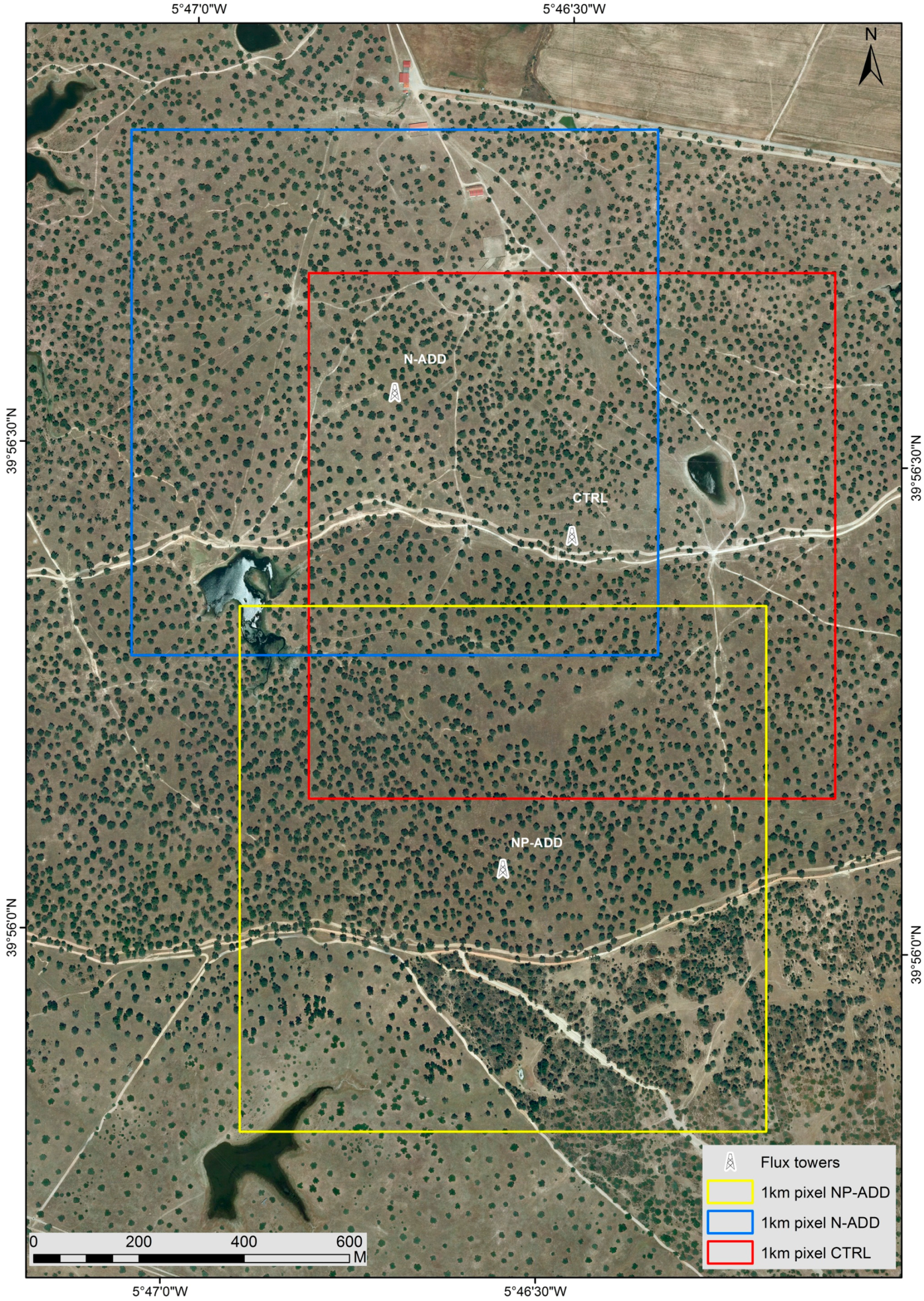
The study area is a managed Mediterranean TGE or “dehesa” located in Las Majadas del Tiétar, in Cáceres, Spain, located at 259 m a.s.l. (39°56′29′′N, 5°46′24′′W) (Figure 1). Climate is Continental Mediterranean with an annual mean temperature of 16.7 °C and annual mean precipitation ~700 mm [32]. In summer, temperature goes over 40 °C and only the 6% of the annual rainfall is accumulated [33]. The tree layer is mostly composed by scattered plants of Quercus ilex subsp. ballota L., an evergreen Mediterranean species; these are separated by 18.8 m (standard deviation, σ = 5.0 m) so that the fractional cover is approximately 20%. Mean tree height is 7.9 m (σ = 0.9 m), mean crown horizontal radius is 4.18 m (σ = 0.9 m) and mean vertical radius is 2.7 m (σ = 0.5 m) [34]. The grass layer is rich in species such as Rumex acetosella L., Erygium campestre L., Erodium cicutarium L. or Erodium botrys (Cav.) with a variable spatial and temporal distribution. Grasses show a strong phenology, they usually peak in spring, senesce by summer, regrow in autumn immediately after the first rainfall and go dormant in winter. Cow grazing induces spatial variability and usually keeps the grass layer shorter than 30 cm.
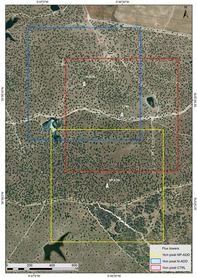
Figure 1.
Location of the flux towers in Majadas del Tiétar. Each square corresponds to a synthetic 1 km pixel centered on each one of the towers.
Three EC flux towers operate in the site. They are included in the FLUXNET research network (http://fluxnet.ornl.gov/site/440, last accessed on 16 May 2017) and monitor a large scale fertilization experiment (MaNiP) [35]. The first tower (CTRL) is operative since 2003; moreover, two additional towers were installed in April 2014. The former one (N-ADD) is located 435 m northwest of CTRL, and the latter (NP-ADD) 645 m on the south of CTRL. The location of the new towers was based on the CTRL tower footprint estimation based on ten years of existing measurements. The main wind directions at the site are east-northeast and west-southwest; therefore, the footprints display along this line and show, especially under daytime conditions, no sampling outside of the fertilized area of interest. Analyses carried out by El-Madany et al. [36] show no overlap between the 80% iso-lines of the footprint climatology for the three towers. Between December 2014 and March 2015, a fertilization experiment was carried out in the surroundings of the N-ADD and NP-ADD towers. An area of about 20 ha was fertilized with nitrogen and phosphorous + nitrogen in the N-ADD and NP-ADD towers, respectively [37].
2.2. Airborne and Ground Hyperspectral Data
Airborne hyperspectral images were acquired using the Compact Airborne Spectrographic Imager CASI-1500i (Itres Research Ltd., Calgary, AB, Canada), operated by the Instituto Nacional de Técnica Aeroespacial (INTA). Data were taken during campaigns between May 2011 and July 2015 supported by the projects BIOSPEC [38], FLUχPEC [39], CEOS-Spain [40], and the EUFAR TA DEHESyrE [41]. Eleven overpasses were selected for this work centered on the eddy flux towers (Table 1). The CASI sensor featured 144 spectral bands between 380 and 1050 nm, with a full width at half maximum (FWHM) of ~5.5 nm. CASI field of view (FOV) is 40°, providing approximately 0.90 m × 1.66 m pixels, which were resampled to 1 m size in the geometric correction. The nearest neighbor resampling was used to prevent spectral mixture. Atmospheric correction was carried out by the data provider using ATCOR-4TM and ancillary measurements of water vapor and aerosol optic thickness using a CIMEL CE318-NE sun photometer (Cimel Electronique, Paris, France) when available. Atmospheric correction was refined using the Empirical Line method [42] and ground spectral measurements of dark and bright calibration targets measured simultaneously to the overpasses using an ASD FieldpsecTM 3 spectroradiometer (Analytical Spectral Devices Inc., Boulder, CO, USA).

Table 1.
Characteristics of the eleven overpasses of the Compact Airborne Spectrographic Imager (CASI) imagery acquired in the Majadas del Tiétar research area.
After atmospheric correction, images were classified using ENVI 5.1 + IDL 8.3.0 (Harris Geospatial Solutions, Boulder, CO, USA). Supervised classification based on Mahalanobis distance allowed discriminating the following classes: “water”, “grass”, “trees”, “shadows” and “soils/roads”, using both the noiseless Hemispherical-Directional Reflectance Factors (HDRF) between 425 and 980 nm and Spectral Vegetation Indices (SVI) (see Table S1 in the Supplementary Materials). Since spectral calibration of the airborne sensor varied between campaigns, HDRF at the center of the bands used for hyperspectral SVI computation was estimated by linear interpolation. In addition, spectral measurements of 25 m × 25 m grass plots were obtained in the surroundings of the three towers simultaneously to the airborne overpasses. Field protocols are described in described in Mendiguren et al. [43]. Additionally, field spectral measurements were acquired in several dedicated campaigns between 2009 and 2015. For each flight campaign, some of the SVI computed from the field spectroscopy measurements collected in the grass plots close to the EC towers were compared to the “grass” airborne derived SVI averaged on a 1 km2 square centered on each tower. The Pearson correlation coefficient (r) and the p-value (p) were used to assess the strength of the relationships.
2.3. Eddy Covariance Data and Footprint Analysis
Carbon dioxide (CO2), water and energy fluxes were measured using the EC technique. Wind velocity components were measured using an ultra-sonic anemometer (SA-Gill R3-50; Gill Instruments Limited, Lymington, UK) and water vapor and CO2 fluctuations with an enclosed-path infrared gas analyzer (LI-7200, LI-COR Biosciences Inc., Lincoln, NE, USA) positioned at 15 m. EC raw data—including the three dimensional wind velocities (u, v, w in m/s), sonic temperature (Ts in K), and dry CO2/H2O mixing ratios—were collected at 20 Hz. Data were processed with EddyPro software (version 5.2.0, LI-COR Biosciences Inc., Lincoln, NE, USA) as described in Perez-Priego et al. [32].
A quality flag was assigned to each half-hourly flux according to Mauder and Foken [44] and Vicker and Mahrt [45]; data flagged as low quality or during rain events were removed from the dataset. Data with low turbulent mixing were identified and discarded from analysis according to the algorithm developed by Papale et al. [46] and implemented in the REddyProc R Package [47,48]. The procedure was applied separately to all the towers and a friction–velocity (u*) threshold of 0.14 m/s was used for further filtering. CO2 fluxes were corrected for CO2 storage using the single point correction according to Greco and Baldocchi [49]. The resulting Net Ecosystem Exchange (NEE) estimates were then partitioned in GPP and ecosystem respiration (Reco) according to Reichstein et al. [50] using the REddyProc R Package [47,48]. From the final dataset, only high-quality GPP data coming from daytime (Global incoming radiation, Rg > 10 W·m−2) were used.
As surrogate of the uncertainty in the GPPhh () was used the random uncertainty of NEE (e) derived from the standard deviation of the marginal distribution sampling of the gap-filling procedure [50]. This methodology represents one way to assess the random error of the NEE [46,51,52]. should account also for the formal propagation of the uncertainty introduced by the determination of the u* threshold used to filter the data with low turbulence conditions (e.g., [46]). However, in this study we did not formally propagate this uncertainty because we are focusing on daytime and mainly on midday fluxes measured with high PAR and; in these conditions, e and NEE are strongly correlated because NEE is dominated by photosynthesis [53]. Additionally, under daytime/midday conditions the u* threshold is usually exceeded and no filtering is applied. was calculated in order to weight a cost function which includes prior information on the model parameters (see Section 2.5). Therefore, for this purpose, the uncertainties in NEE and GPP are comparable because they are strongly correlated.
Footprint climatology was computed using a modified version of the 2-D model developed by Hsieh et al. [54] and updated by Detto et al. [12]. Footprints were integrated in periods of 30 min, similarly as the EC variables. Specific details can be found in [55] and El-Madany et al. [36].
2.4. Eddy Covariance Footprint and Hyperspectral Data Integration
For each overpass, optical and footprint climatology data were combined in a period of ±15 days around each airborne campaign. To do so, half-hourly 2-D probability distribution functions representing the contribution of each pixel to the measured carbon fluxes (Pfp) were convolved with imagery. This provided a footprint-weighted spectrum (Sfp), this is, the averaged optical properties of the footprint area contributing during that specific time to the EC system. First, Sfp only weighted the different vegetated classes (“grass” and “trees”) according to their probability of occurrence in the footprint area, their spectral properties and the Pfp of each pixel. In a second step, convolution was applied including also “shadows/water” and “soil/roads” classes in order to analyze their impact on Sfp and the later estimation of GPP. Spatial convolution was only applied to daytime data and it was limited to a 1 × 1 km2 square centered on each EC tower, which was large enough to contain EC footprints during daytime. Since the Pfp spatial resolution—5 m—was coarser than the one in the images, the corresponding Pfp value of each pixel was linearly interpolated to pixel coordinates (x, y). Interpolation is suitable for smooth surfaces as those presented by Pfp. The half-hourly Sfp of a single class (j) can be calculated as shown in Equation (1):
where λ stands for wavelength and S is a n-by-m matrix containing the HDRF (or SVI) of the m pixels selected in the surrounding of the EC tower, and n is the number of spectral bands or indices. Pixels are defined by their Cartesian coordinates. Pfp is a 1-by-m vector with the pixel probability of contribution to the measured fluxes at a given time (t). Since Pfp,j will correspond exclusively to the pixels of a single class, it is normalized to 1. Resulting Sfp is an n-by-1 vector with the spectrum (or the SVI) of the vegetation contributing to the fluxes at that time, and as observed from a remote sensor. It should be noted that part of the grass is always occluded by three crowns.
Similarly, the Sfp of different k classes (Sfp,mix) can be combined as follows:
where q stands for the individual length of the Pfp of each class k. This way, the Sfp of the category “vegetation” is built combining the respective spectra or SVI of the classes “grass” and “trees”. In addition, the Sfp including all the classes—labeled “all”—was computed in this way.
In this approach, the same image is used for a period of 1 month; this assumes that optical properties of land surfaces did not vary within the ±15 days around each campaign. This assumption is unrealistic, but can be used to assess the impact of the temporal mismatch between optical and flux data on the estimation of GPP. To do so, in Section 2.5, we analyze GPP models performance over time to see if errors increase as a function of the temporal distance to the flight campaign.
In addition, we computed the average spectral signature and indices of squared synthetic pixels centered on each EC tower using all the classes. These synthetic pixels had sizes of 250, 500 and 1000 m (spectral data are labeled as SP250, SP500 and SP1000 respectively). In Section 2.5, we compare the performance of models predicting GPP using spectral information from the different Sfp and SP computed in order to assess the impact of the spatial mismatch between EC and RS footprints.
2.5. GPP Models: Definition, Inversion and Analysis
According to Monteith [2], GPP results from the product of the incoming PAR, the fraction of it absorbed by green vegetation (fPAR) and the Light Use Efficiency (ε) (Equation (3)). Optically-based GPP predictive models can be developed using SVI as proxies of the parameters in the Monteith’s model [4].
In this work, we fit and test the performance of four different GPP models considering different degrees of complexity, and of spatial and temporal mismatch between optical and EC observations. The first three models (MOD1–MOD3) make use of PAR and optical information and have already been tested by several authors using field spectroscopy data [32,56,57]. These models replace Monteith’s equation parameters by linear functions of SVI. We used the Normalized Difference Vegetation Index (NDVI) [58] (Equation (4)) and Photochemical Reflectance Index (PRI) [59] (Equation (5)) to represent fPAR and ε respectively. Moreover, we assessed the performance of different PRI formulations designed to minimize the effect of vegetation structure and pigment contents in the estimation of ε. Specifically, we tested PRI515 (Equation (6)) [60] which was found less sensitive to canopy structure than PRI; the Normalized PRI (PRInorm, Equation (7)) [61] which was related to water stress and normalizes for different canopy chlorophyll concentrations; and the Calibrated PRI (CPRI, Equation (8)) [62] also normalized by pigment content. Notice that all PRI-based indices are formulated in such a way that they are positively related with ε.
where RDVI is the Renormalized Difference Vegetation Index [63].
where mNDVI705 is the Red-Edge Normalized Difference Vegetation Index [64].
The fourth model (MOD4) is based on the algorithm of the MODerate-resolution Imaging Spectroradiometer (MODIS) GPP product (MOD17A2) [65]. MOD4 models the ε parameter as the product of the maximum ε (εmax) and a scalar ranging between 0 and 1 that expresses photosynthetic down-regulation; the last is formulated combining linear ramp functions of vapor pressure deficit (VPD) and air temperature (Tair) (Equation (9)).
where VPDmax and TMINmin are the maximum VPD and the minimum Tair values at which photosynthesis is completely down-regulated (ε = 0). Complementarily, VPDmin and TMINmax are the minimum VPD and the minimum Tair at which photosynthesis is not regulated (ε = εmax). In addition, fPAR is described by the Beer’s law (Equation (10)) depending on an extinction coefficient (k) and the Leaf Area Index (LAI) [66]; the second was modeled using a linear function of NDVI (Table 3). As the MOD17A2, we assume k = 0.5 [65].
Table 2 shows the parametric equations of the models fit against observed half-hourly footprint-weighted SVI, GPPhh and micro-meteorological data (PAR, VPD and/or Tair). PAR was assumed to be the 45% of Rg [65] measured in the EC towers.

Table 2.
Optically-based Gross Primary Production (GPP) parametric models inverted against observed half-hourly GPP (GPPhh) and micro-meteorological variables.
The least square nonlinear curve-fitting optimization method implemented in the Matlab® function LSQCURVEFIT. In addition, bootstrap technique [67] with 500 subsamples was applied to quantify the uncertainty of the estimated model parameters. Parameter constrain was only applied to MOD4—the MODIS algorithm—where a4 and a5, representing TMINmin and TMINmax, respectively, were bounded in the ranges (−15, 50) and (0, 50) each with a uniform distribution. Parameters a1–3 representing εmax, VPDmax and VPDmin, respectively, as well as a6—the NDVI-LAI slope—were forced to be larger than 0. In addition, the large equifinality existing between εmax and fPAR was handled by imposing prior information of model parameters a6–7 describing the NDVI–LAI relationship. To do so, a linear model was fit using the averaged data from 16 field campaigns held during the FLUχPEC [39] project. In each campaign, approximately ~13 plots of 25 m × 25 m were sampled. Grass vegetation samples and field spectroscopy data were acquired as described in Mendiguren et al. [43]; however this time only green fraction of LAI was used. Tree LAI was estimated ~1.426 m2/m2 using hemispherical cameras [68] and assumed stable over time. Tree crown NDVI was the mean NDVI of the “trees” class from all the CASI images within the 1 km pixel centered on each tower. “Grass” and “trees” variables were linearly combined with a proportion of 100% and 20%m respectively [69].
For MOD1–MOD3, the cost function used for the inversion was the sum of the squared differences between calculated and predicted GPPhh. For MOD4, the cost function accounted for the prior information in coefficients a6–7 and was computed as in Jacquemoud et al. [70] (Equation (11)):
where g is the number of observations, GPPhh,i and GPPpred,i are each observed and predicted half hourly GPP, and is the corresponding uncertainty of GPPhh (see Section 2.3). In the second term of the equation, aj are the parameters retrieved by model inversion, is the model parameter estimated using independent data, and the corresponding uncertainties of the priors. These are the coefficients of the abovementioned NDVI-LAI relationship. Errors of the linear model fit were propagated to obtain the 95% confidence intervals of the coefficients, and these converted to a standard deviation assuming a normal distribution.
To assess the impact of temporal mismatch between optical and EC data on GPPhh estimation, models were fit with two different datasets. The first is the “Flight” dataset (and models), and only makes use of all the Sfp and EC data acquired the same day of the flight campaigns. “Flight” models predicted GPPhh for the ±15 days surrounding each flight campaign. Within this period we expect that changes in vegetation—not tracked by updated imagery—could lead to larger errors far from the day of the campaigns. For comparison, we fit 30 “Daily” modes using all the Sfp and EC data of the eleven overpasses corresponding to each single day of the period. On one side, this allows to evaluate model robustness against varying meteorological conditions within a narrow time window around the campaigns, while vegetation status can be assumed stable. On the other, further in time from the imagery acquisition, this could reveal model sensitivity to changes in vegetation properties which are not recorded by frequent flight campaigns. The impact of these changes would be assessed via model performance degradation and comparison between “Daily” and “Flight” models. For the comparison of the model performances, we computed the coefficient of determination R2, the Relative Root Mean Squared Error (RMSE) and Akaike’s Information Criterion (AIC) [71]
Partial correlation analysis was used to assess if differences between the variables involved in the models could explain the errors in predicted GPPhh. To do so, we computed the difference (D) between the value of each variable with the value shown the same half-hour during the day of each flight campaign (Equation (12)). This was done for all the days in the study period. D was calculated for the GPPhh, footprint-weighted NDVI (NDVIfp), the different versions of PRI (PRIfp), PAR, time (t) and the ration ratio Tair/VPD—which should be related to εstress according to the MODIS algorithm.
where x is any of the abovementioned variables and d is the number of days to the date when images were acquired and the subscript “hh” means a half hour period of the day an i ∈ (−15, 15).
3. Results
3.1. Airborne Hyperspectral Imagery
Image classification allowed separating the two different vegetation layers and the non-vegetated surfaces. Table 3 shows the percentage per category within the 1 km2 square centered on each EC tower and date: “grass” represents between 68.42% and 79.49% of the surface as observed by the sensor, whereas “trees” represent between 13.83% and 21.55%. “Soils and roads” coverage is lower than 2%. In addition, “water and shadows” range between 3.98% and 11.55%.

Table 3.
Frequency of the different classes in the airborne imagery.
Figure 2 shows the mean spectra of the vegetation classes separated (Figure 2a,b), mixed (Figure 2c) and of all the classes (Figure 2d). As can be observed, “grass” (Figure 2a) shows a large variability, whereas “trees” (Figure 2b) optical properties are more stable. This is in agreement with the phenological behavior of each class. Since “grass” is more abundant, it governs “vegetation” HDRF variability, whereas the remaining classes have a low effect. The figure also shows that the differences between grass spectral features of the three towers increase in 2015 after fertilization.

Figure 2.
Mean spectra of different covers within a 1 km2 square centered on the Eddy Covariance (EC) towers: (a) Grass; (b) Trees; (c) Vegetation (grass + trees); and (d) All covers.
3.2. Eddy Covariance and Optical Data
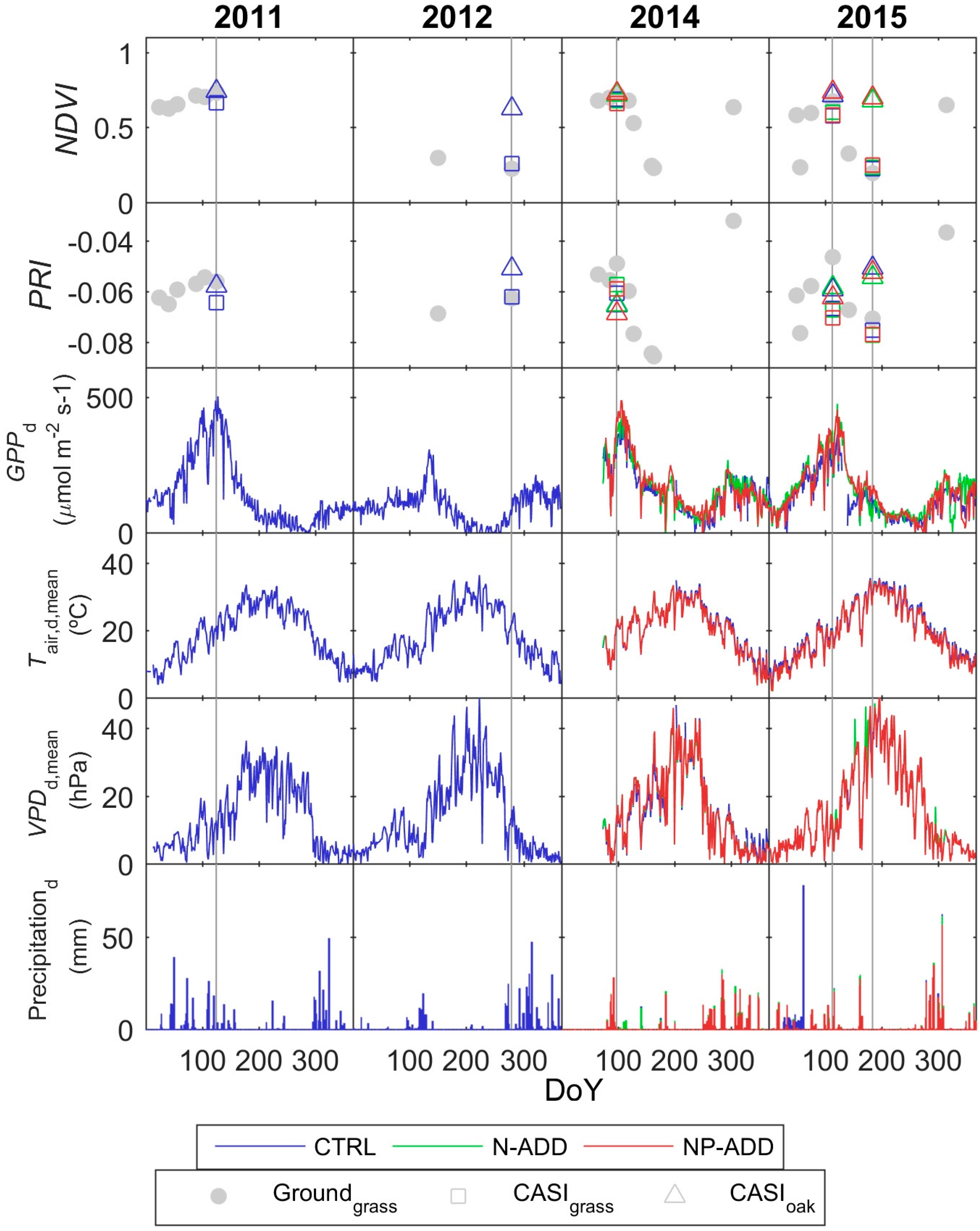
Figure 3 shows the optical and flux data acquired during the flight campaign periods. NDVI and PRI data are shown in the first two rows (Figure 3a,b). Indices derived from field spectroscopy data acquired during several ground campaigns in 25 m × 25 m plots are shown as example of the temporal dynamics in the ecosystem. In addition, the SVI derived from the mean spectra of “trees” and “grass” covers in the 1 km2 square centered on each tower (Figure 2) are shown. “Grass” NDVI derived from ground and airborne sensors are similar, and vary more than trees NDVI along the year. “Grass” NDVI derived from CASI and ground measurements were strongly related (r = 0.99, p < 0.05), whereas the same relationship was weaker for PRI (r = 0.69, p < 0.05). CASI “grass” PRI was related positively with NDVI (r = 0.74, p < 0.05); which was confirmed by field spectroscopy data (r = 0.88, p < 0.05). On the contrary, the same indices presented a negative relationship (r = −0.69, p < 0.05) in CASI “trees”. For all the “vegetation” pixels, both indices were positively correlated (r = 0.65, p < 0.05). The four formulations of PRI presented different degrees of correlation with the original index. For “grass” (and “vegetation”) pixels, all the indices were significantly correlated (p < 0.05); PRI was positively correlated with PRI515 and PRInorm, and negatively with CPRI. For “trees” pixels, PRI was positively related with PRInorm, and negatively with PRI515 and CPRI (p < 0.05).
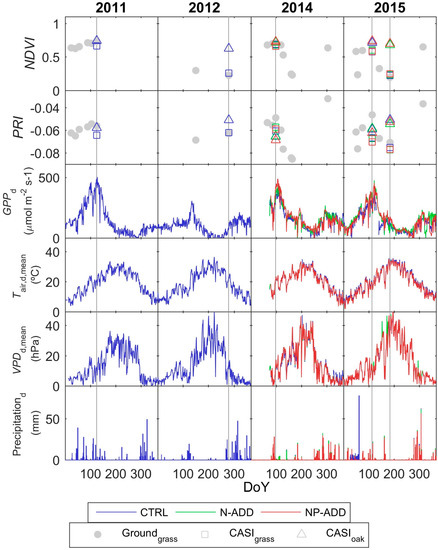
Figure 3.
Optical (spectral vegetation indices), flux (daily accumulated GPP) and meteorological (daily mean air temperature (Tair), vapor pressure deficit (VPD) and daily accumulated precipitation) data acquired in the site of Majadas del Tiétar in the years of the airborne flight campaigns.
Figure 3c–f shows the yearly trends of daily meteorological variables: daily cumulated GPP (GPPd) (Figure 3c), daily mean Tair (Tair,d,mean) (Figure 3d), and VPD (VPDd,mean) (Figure 3e). GPPd peaks in spring, reaches minimum values during the summer and recovers during autumn after the onset of the rainfall. There is a large inter-annual variability in GPP; 2012 was the driest year, with low precipitation in winter and spring and GPPd presented low values, except for a brief rise in spring. Autumn precipitation triggered a recovery of the vegetation activity more pronounced than in previous years. More precipitation was observed in spring in 2011, 2014 and 2015; this was followed by a quick drought in late spring/early summer and then by a later recovery after autumn rains. Some differences in GPPd can be observed between the three towers in 2015, which are larger after nutrient addition [37].
3.3. Footprint Climatology and Hyperspectral Data Integration
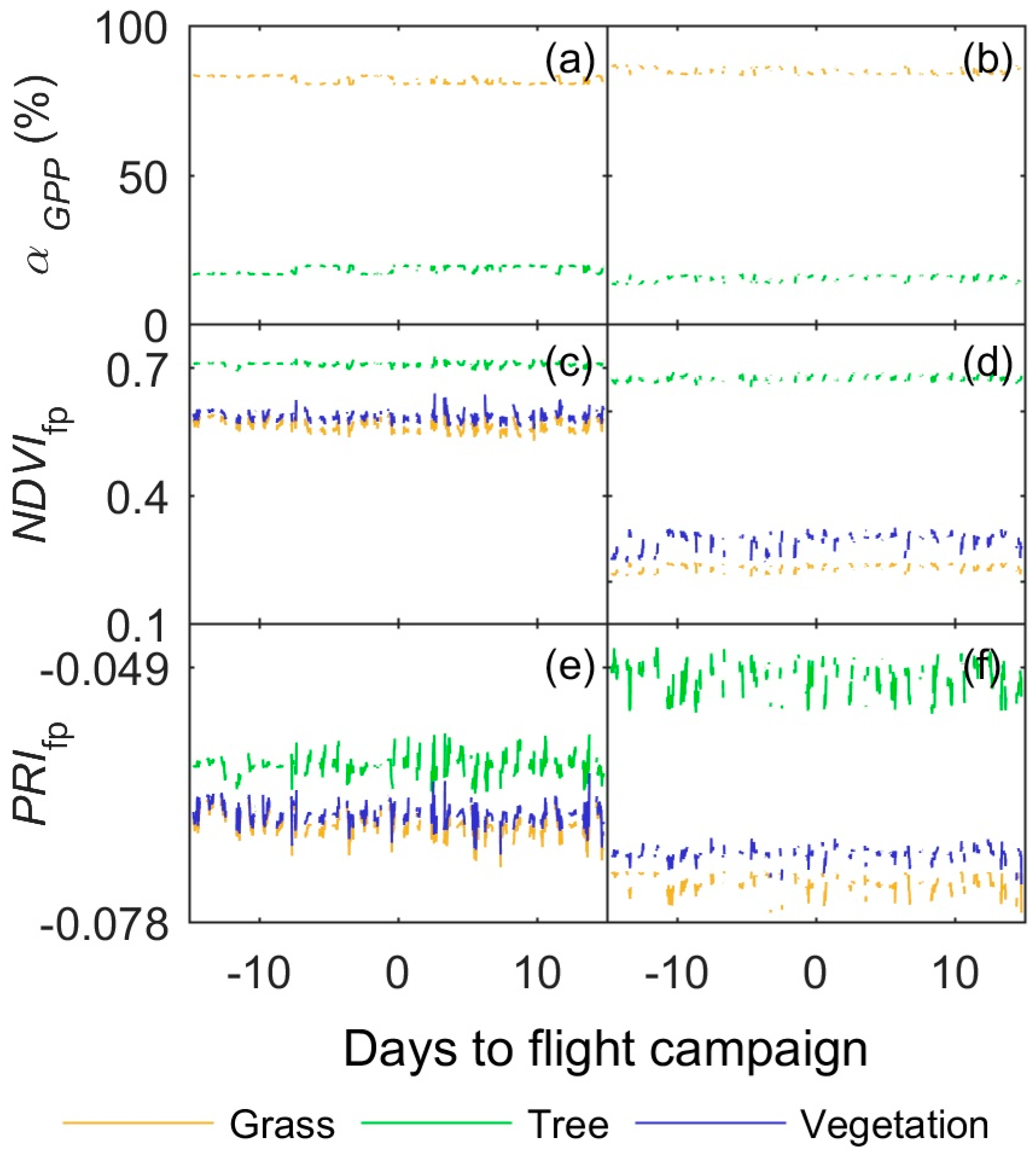
The convolution of the estimated Pfp on the hyperspectral images provided not only weighted representative spectra of vegetation contributing to half-hourly fluxes; but also the vegetation classes’ relative contribution or weight within the EC footprint (αGPP)—as observed from a remote sensor. An example is shown in Figure 4a,b, where the values of NVDIfp (Figure 4c,d) and PRIfp (Figure 4e,f) of each vegetation class separated and combined are presented. Data shown correspond to the 31 days selected around the flight over the CTRL tower in two very different phenological stages: April 2015 (left column) and July 2015 (right column). αGPP (Figure 4a,b) is similar for the different dates, remaining stable in average for each of the 31 days of the study period. αGPP temporal variability is governed by footprint size and direction. Grass NDVIfp shows large differences between the two dates; though much lower for trees. On the contrary, “trees” PRIfp varies more between dates than “grass” PRIfp.
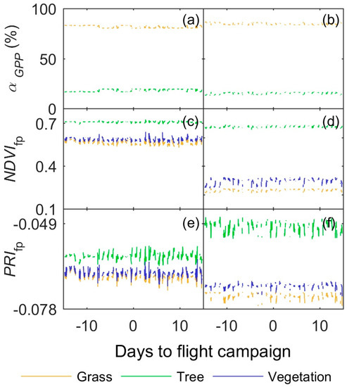
Figure 4.
Footprint induced variability in optical signals acquired over the control (CTRL) tower on: 23 April 2015 (a,c,e); and 3 July 2015 (b,d,f), on the relative area of the different vegetation covers contributing to: GPPhh (a,b); the Normalized Vegetation Index (NDVIfp) (c,d); and the Photochemical Reflectance Index (PRIfp) (e,f).
As shown in Figure 4, NDVI footprint-induced variability is much lower than changes induced by phenology. For each overpass, the standard deviation of each SVI is calculated within the 31 days study period. The averaged standard deviation for all the overpasses is lager for “grass” (subindex “g”) ( = 1.52) than for “trees” (subindex “t”) ( = 0.61). However, when NDVIfp of both categories are mixed as a function of αGPP (subindex “veg”), variability increases ( = 1.72). In the case of PRI, “grass” and “trees” variability is equal ( = 0.17) and reduces when mixed ( = 0.15). Footprint-induced variability was also related to vegetation status in some cases. Considering the 11 overpasses, “grass” NDVIfp was positively related to standard deviation (r = 0.77, p < 0.05), whereas “trees” NDVIfp was negatively related to (r = −0.55, p < 0.10). “Grass” PRIfp was related to (r = 0.71, p < 0.05), whereas in “trees” the relationship was not significant. For “vegetation” pixels, PRIfp was significantly related to (r = 0.60 p < 0.10).
3.4. GPP Models Performance
Table 4 shows the median model coefficients and the corresponding 95% confidence intervals estimated by Bootstrap. In models MOD1–MOD3, coefficient a1 is almost always positive, suggesting a direct relationship between NDVI and fPAR. However, in MOD3-PRI515 the coefficient is negative and the confidence interval overlaps negative values suggesting a slope close to 0. In MOD3, the median value of coefficient a3 is always positive, suggesting a positive relationship with ε. However, confidence intervals overlap 0 in all the cases. For MOD4 inversion, a linear model predicting LAI from NDVI was fit (r2 = 0.72, RMSE = 0.28 m2/m2); prior estimates of a6 and a7 coefficients were (2.826, −0.430) with respective uncertainties (0.544, 0.359). Estimated coefficients were close to the priors with narrow confidence intervals. The remaining coefficients in MOD4 can be compared to values used by MODIS GPP algorithm for Savannas [65]. Estimated coefficient a1 (representing εmax) median is 1.644 gC/MJ similar to the MODIS εmax (1.206 gC/MJ). Coefficients a2 and a3 represent VPDmax and VPDmin respectively, the first is larger than the value used in MODIS (31.0 hPa) and the second is lower than the MODIS parameter (6.5 hPa). Coefficients a4 and a5 representing TMINmin and TMINmax respectively are quite close to MODIS parameters (−8 °C and 11.39 °C, respectively). In addition, VPDmax and TMINmax present wide confidence intervals.

Table 4.
Parameters with 95% confidence intervals for the different models retrieved using the “Flight” dataset.
Table 5 shows the statistics R2, RRMSE and AIC for the different model fits using the “vegetation” and “all” covers from the “Flight” dataset. Footprint and pixel-based approaches are compared for synthetic pixels of different size. Model fits using footprint climatology and “vegetation” pixels (Sfp,veg) show similar performances in terms of R2 and RRMSE. MOD1 achieves the lowest R2 (0.65) and RRMSE (35.89%), but also the largest efficiency. MOD2–MOD3 present similar errors and fits (R2 ϵ (0.67–0.68); RRMSE ϵ (36.71–37.66)), and thus the most efficient model is the simplest one (MOD2). MOD3-PRI515 achieves best performance in all the statistics. MOD4 presents the largest R2 (0.72) and an intermediate RRMSE (37.19%), as well as the lowest efficiency. The combination of footprint climatology without discrimination of non-vegetated pixels (subindex “all”) (Sfp,all) reduces the performance of all models, where MOD3-PRI515 and MOD4 are the least sensible. In the table, the statistics of model fits using all the pixels within synthetic squared pixels centered on each tower of different sizes—SP250,all, SP500,all, SP1000,all—present similar performances than Sfp,all. In most cases R2 increases; RRMSE either increases or decreases and in all cases AIC increases.

Table 5.
Statistics for the different model fits using the “Flight” dataset as well as the weighted spectral signature of vegetation covers or different synthetic pixel sizes.
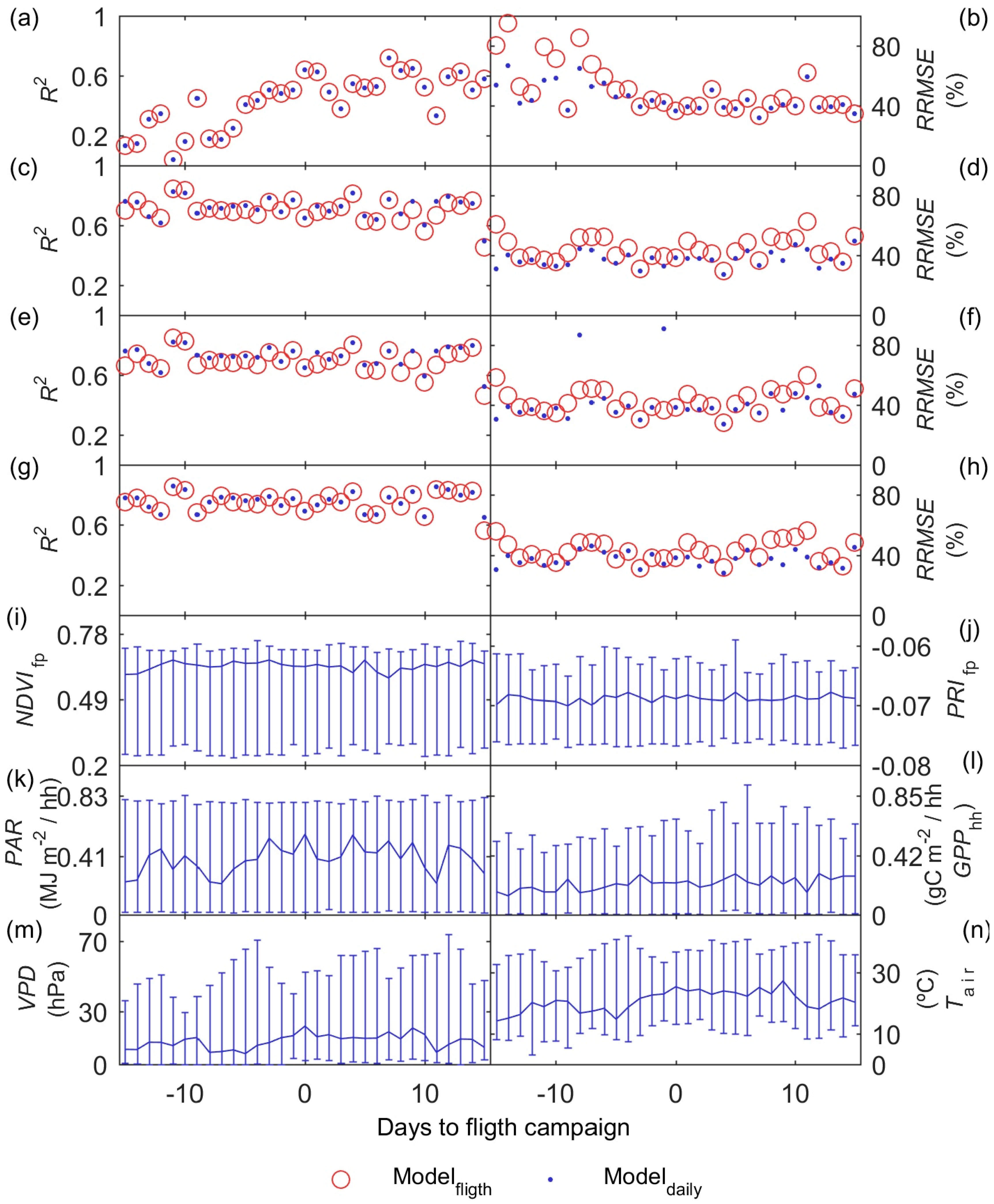
Figure 5a–h shows R2 and RRMSE of the different models using the Sfp,veg dataset. In each subplot, the statistics of the “Flight” and “Daily” models are compared. For simplicity, only results of MOD-PRI are shown. Different PRI formulations show almost identical performances. In addition, Figure 5i–n presents the range of variation and the median of the variables used to fit the models using daytime data of each of the “Daily” datasets, which integrate data from the 11 overpasses. As can be observed, in the ±15 days period around the flight campaigns, the spectral indices NDVIfp (Figure 5i) and PRIfp (Figure 5j) as sampled from the same image show small variations in terms of range or median values; nonetheless the second is more variable. Meteorological variables show larger variability: PAR (Figure 5k) keeps ranges relatively constant in the period analyzed while the median shows large variations. Maximum median values match airborne campaigns. VPD (Figure 5m) and Tair (Figure 5n) show larger variations both in median and ranges compared to PAR. GPPhh (Figure 5l) also shows a pronounced variability and maximum values not always occur during the campaigns. Predicted-observed statistics compare the performance of two models fit using the “Flight” and “Daily” datasets. MOD1 R2 (Figure 5a) are the same for the “Flight” and the “Daily” models since these are just a linear combination of one predictive variable. However, RRMSE (Figure 5b) differ and show that “Daily” models perform better in periods where meteorological conditions were different compared to those of the day of the flight. Differences are mainly noticed in the period before flight campaigns, when also maximum GPPhh reaches lower values than the rest of the month considered in the analysis. For MOD2 (Figure 5c,d), MOD3-PRI (Figure 5e,f) and MOD4 (Figure 5g,h), “Flight” and “Daily” R2 and RRMSE differences are smaller.
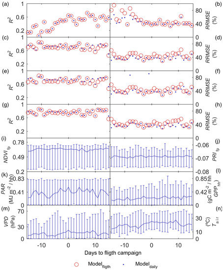
Figure 5.
Predicted-Observed statistics of the models: MOD1 (a,b); MOD2 (c,d); MOD3-PRI (e,f); and MOD4 (g,h). Daily ranges of variation and median of the input variables: NDVIfp (i); PRIfp (j); photosynthetically active radiation (PAR) (k); and measured: GPPhh (l); VPD (m); and Tair (n).
Figure 6 shows a deeper analysis on these effects. Each column summarizes data from a single flight campaign. For comparison, we only present the campaigns where the three eddy flux towers were operative: April 2014 (first column), April 2015 (second column) and July 2015 (third column). Only “Flight” and “Daily” RRMSE of the simplest (MOD1) and the most complex (MOD4) models are shown in the first two rows. Below, PAR (Figure 6g–i), Tair (Figure 6j–l), VPD (Figure 6m–o), GPPhh (Figure 6p–r) and footprint-weighted NDVIfp (Figure 6s–u) are presented. Results show that “Flight” MOD1 (Figure 6a–c) and MOD4 (Figure 6d–e) RRMSE increase, compared to “Daily” models, in periods when meteorological variables largely differ from those found the same days of the airborne campaigns. The days following the flight campaign in April 2014 are more similar than in April 2015; this campaign was surrounded by cloudy days where PAR, Tair and VPD dropped, increasing errors as well as the distance between “Flight” and “Daily” RRMSE. In general, MOD1 is more sensible to these changes since it does not include meteorological variables. In July 2015 RRMSE is rather sensitive to changes in Tair and VPD, and it is remarkable that MOD4 has difficulties to predict GPPhh under large VPD conditions. In addition, on these dates, the metric RRMSE is more sensitive to errors since GPPhh is low.
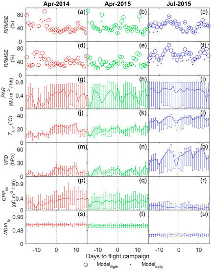
Figure 6.
MOD1 RRMSE (a–c); and MOD4 RRMSE (d–e). Ranges and median values of: PAR (g–i); Tair (j–l); VPD (m–o); GPPhh (p–r); and NDVIfp (s–u). In each column, data correspond to the three overpasses (one on each eddy flux tower) of a single date: April 2014 (first column), April 2015 (second column) and July 2015 (third column).
3.5. GPP Models Error Analysis
To understand what factors drive model performances, model errors (GPPhh,pred − GPPhh,obs) are compared to the distance between the half-hourly values of the variables: NDVIfp (DNDVI); the different formulations of PRIfp (DPRI), PAR (DPAR), Tair/VPD (DTair/VPD), and GPPhh (DGPP); and the distance in days to the flight campaigns (Dt). Partial regression coefficients (rerr|D) and the corresponding p-value are presented in Table 6. In all the models, error values are inversely related to DGPP which means that the models underestimate GPPhh when it is larger than the day of the flight. DPAR explains a substantial part of the errors in all the models; rerr|D is positive meaning that GPPhh is underestimated when PAR is lower than the day of the flight. The remaining variables show lower explanation power. Dt is not significant in all the cases; errors are inversely and non-significantly related to DTair/VPD in all the models but MOD1 and MOD4 where relationships are positive and significant. SVI rerr|D are also low and in general negative for PRIfp and positive for NDVIfp.

Table 6.
Partial correlation coefficients and significance between GPPhh prediction errors and the Euclidean distance between each half-hourly input variable the day of the flight campaigns and the surrounding days.
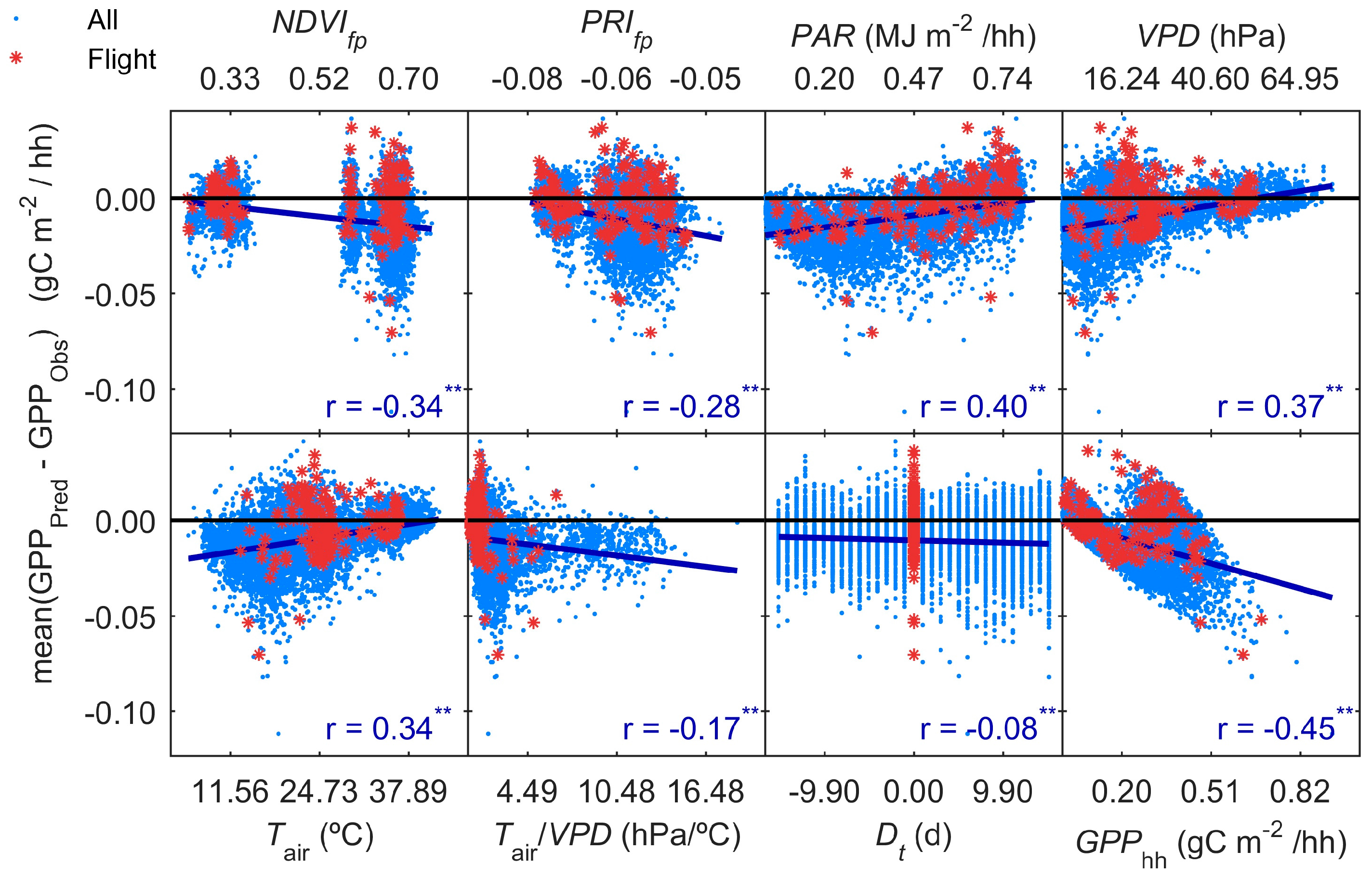
To better understand the previous results, we analyzed the direct dependence of errors on model variables (Figure 7) and their differences with respect to the days of the flight campaign (Figure 8). Figure 7 shows the averaged error of MOD2–MOD4 vs. the different variables involved in the models. MOD1 is excluded since it behaves differently than the others. Error range increases with NDVIfp and PRIfp while Pearson r is negative. GPPhh is underestimated in situations with low-mid PAR, VPD and Tair values (r ≥ 0.34). Both over and underestimation occur at low Tair/VPD values, and underestimation at mid-high Tair/VPD. In addition, underestimation is higher at high GPPhh. Time to the flight day show a very weak but significant relationship when errors from MOD2–MOD4 are averaged, which was not observed for each individual model.
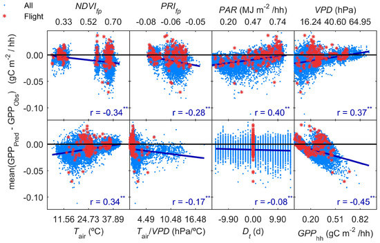
Figure 7.
Mean error of MOD2–MOD4 vs. different variables. The adjusted linear model and Pearson correlation coefficient of the whole dataset are shown with the respective significance degree (** p < 0.05; * p < 0.10). In addition, data corresponding of the date of each flight are flagged.
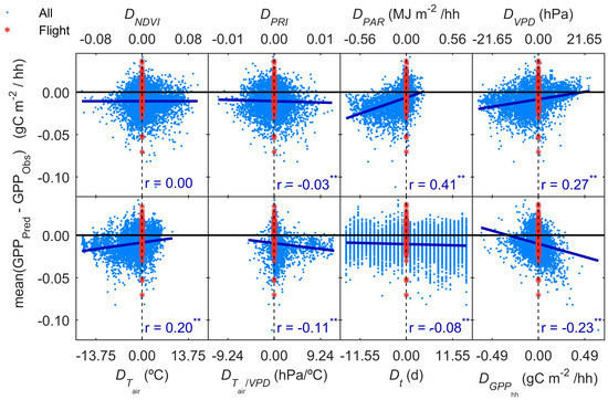
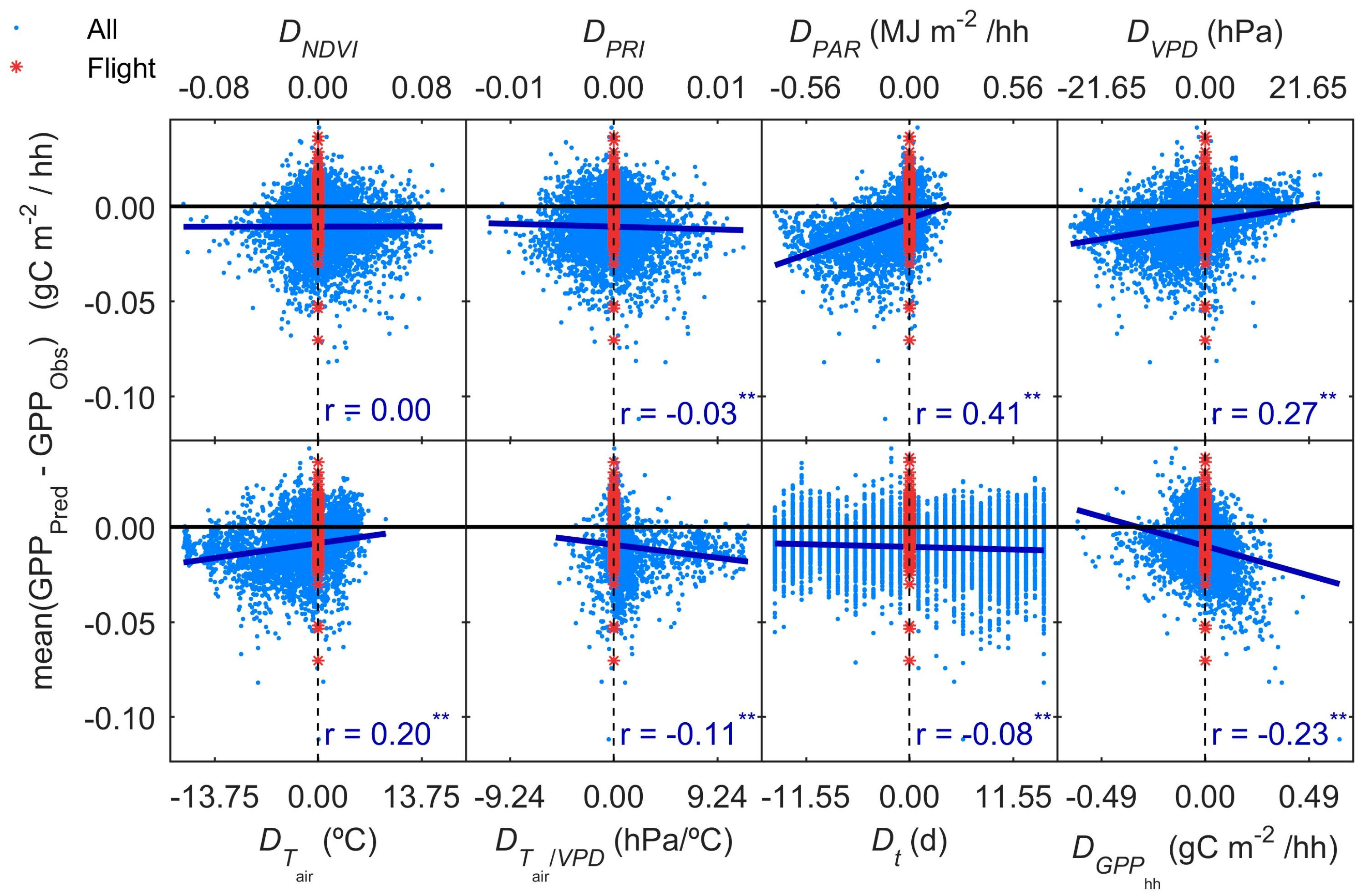
Figure 8.
Mean error of MOD2–MOD4 vs. the difference of different variables respect to their values each half-hour the days of the flight campaigns. The adjusted linear model and Pearson correlation coefficient of the whole dataset are shown with the respective significance degree (** p < 0.05; * p < 0.10). In addition, data corresponding of the date of each flight are flagged.
Similarly, Figure 8 shows the averaged errors from MOD2–MOD4 vs. the differences previously used in the partial correlations analysis (MOD1 errors are excluded since behaved differently). As can be seen, GPPhh is underestimated in conditions of lower PAR (DPAR < 0), lower VPD and lower Tair than those found the day of the flights, as well as when GPPhh and Tair/VPD are larger. However, the largest errors are found for Tair/VPD under conditions very similar to those of the flight. Footprint-weighted SVI and time distance to the flight show little effect.
4. Discussion
In this work, we assess the effect of different sources of uncertainty in the optically-based modeling of GPPhh in a Mediterranean TGE. Different models based on optical and meteorological data have been tested to predict GPPhh. Despite using detailed EC footprint climatology to spatially match spectral and flux data, none of the models achieved high precision (RRMSE ~ 36%). With these results, we try to answer the two scientific questions posed at the end of the Introduction.
- (i)
- Results show that, even in this ecosystem, relatively heterogeneous at the small scale but homogeneous at larger scale, the impact of the spatial mismatch between EC and RS footprints on the estimation of GPP is not very important. This means that when footprint climatology and RS pixels present similar characteristics, the spatial mismatch between EC footprint and optical footprint can become less relevant than other sources of variability or uncertainty. In our case, the impact of non-vegetated surfaces is low, and trees and grasses are quite homogeneously mixed at footprint and mid-low spatial resolution RS scales (Table 3, Figure 4). However, we hypothesize that the mix of trees and grasses hamper the accurate modeling of photosynthesis and GPPhh in this type of ecosystem with simple light use efficiency approaches or semi empirical models.
- (ii)
- Results also suggest that the impact of the temporal mismatch between RS data (i.e., flight overpass) and fluxes was low. Only slight increases of the errors were related to this mismatch. In general, “Daily” and “Flight” models showed similar performances as soon as they included PAR (MOD2–MOD4), and differences in RRMSE were sensitive to variations in meteorological variables. In our site, grasses show a strong phenological variability which might overrule trees contribution to RS and EC signals. Therefore, we hypothesize that larger accuracies or continuous acquisition of RS data would be needed to determine the actual impact of changes in vegetation properties between consecutive mid-temporal resolution remote observations.
We analyzed models of increasing complexity, expecting them to become more sensitive to spatial and temporal mismatches between RS and EC data. However, performance increased only slightly once models accounted for incoming PAR (MOD2–MOD4). In addition, errors were related to the magnitude (Figure 7) and/or the differences between the values of meteorological and optical variables when comparing “Flight” and “Daily” datasets (Table 6, Figure 8). This questions how accurately did models manage to represent ε and/or fPAR. Failure to properly model these variables could be explained by the combination in this TGE of two different types of vegetation that present very different dynamics, variabilities and functions. Grass presents quite dynamic seasonal cycles dominated by LAI and pigment content variations, whereas evergreen trees rather modify ε and fPAR than LAI.
Failure in the modeling of light use efficiency can be differently explained for each model. MOD1–MOD2 ignore ε and therefore poor performance was expected. However, MOD1 achieved lowest RRMSE and maximum efficiency. Nonetheless, this model splits predictions in two groups of extreme GPPhh values (not shown) and is not sensitive to intermediate values of GPPhh. MOD3, includes ε as a linear function of different formulations of PRI. Such relationships have been mainly found when comparing instantaneous PRI-based indices with daily or midday light use efficiency [56,57,72,73,74,75], or when simultaneously observing similar canopies under contrasting stress levels [60,76,77]. However, estimation of instantaneous ε is complex and has been tackled using continuous multi-angular observations [78,79]. Nonetheless, empirical and theoretical works question to what extent the facultative component of PRI rather than structural, directional and pigment-pool effects can induce these relationships [76,80,81,82]. In our case, none of the PRI formulations added significant information about light use efficiency, whereas Perez-Priego et al. [83] found that a PRI-based index was a good predictor of grass GPP in the same ecosystem. The combination of grass and sparse trees could hamper any PRI-based modeling of ε in our case. Trees PRI showed large variability which suggests that crown geometry and self-shadowing could operate as a strong confounding factor. Overall, results suggest that in a heterogeneous ecosystem as a TGE, PRI snapshots might be rarely linked to instantaneous ε, and that more advanced approaches should be used to account for structural and pigment-related effects of trees and grasses. MOD4 slightly raised R2 but also was the least efficient model. Large equifinality between fPAR and εmax led to senseless coefficients (not shown) and had to be constrained using prior knowledge of the NDVI-LAI relationship. Some authors already reported the sensitivity of this parameter, and suggested modifying εmax to improve GPP prediction [84,85]. Retrieved parameters are quite close to those estimated for MOD17A2 in Savanna ecosystems. Large confidence intervals found in VPD and Tair limits could be explained by covariance of these variables [65]; in fact MODIS, VPD limits were independently parameterized from the BIOME-BGC model [86]. In addition, Chen et al. [85] used soil water content to stabilize solutions. Retrieved VPDmax doubled the MODIS value, which could mean that, in this site, photosynthesis does not stop under high VPD. This hypothesis should be handled carefully since the assumption of linear relationships between εstress and Tair and VPD might be unrealistic, and others could be more suitable [87,88]. Nonetheless, larger tolerance to VPD could be explained in this site by the fact that trees have access to deep water reservoirs. In fact, a significant reduction of leaf water content in these trees was only observed during an extremely dry summer [89]. Finally, despite including meteorological variables, MOD4 performance was comparable to other models. This suggests that ε and fPAR should be separately modeled at least for the main vegetation types of the ecosystem (tress and grasses). In addition, other variables better describing their respective resources availability such as soil water content could improve modeling [85,90] and contribute to separate the different physiologies. The authors recognize the limitations of the semi-empirical approaches and the relatively small dataset size (11 images). However, in the case of MOD4, the similarity to MODIS parameters suggests high robustness.
The description of fPAR provided by the different models might also result inadequate in TGE and structurally complex ecosystems. The SVI-based [4] or the Beer-Lambert law-based (Equation (11)) approaches might require that the assumption of homogeneity and random distribution of leaves helds [91]. However, dispersed trees add a geometric component to scattering [92,93] that modifies radiation distribution over vegetation. In fact, NDVI-fPAR relationships of different nature have been found in grass savannas [94,95]. Background, directional effects and pixel heterogeneity could also compromise the estimation of fPAR [96,97]. SVI not used in this work have been proposed to minimize some of these effects, as the Soil Adjusted Vegetation Index [98] or the Enhanced Vegetation Index [99] and are prescribed for heterogeneous landscapes such as TGE [100]. In other cases, indices maximizing sensitivity to canopy chlorophyll such as the MERIS terrestrial chlorophyll index (MTCI) were reported as better estimators of fPAR [56,101]. However, SVI-based fPAR modeling does not explicitly describe radiation interaction in a heterogeneous 3-D structure, and only more advanced approaches could robustly improve fPAR representation in TGE ecosystems. In this work, error analysis reveals that GPPhh is underestimated in a wide range of sun zenith angles and at mid-low PAR conditions, but that overestimation is maximum at low sun zenith angles (<30°), and large PAR conditions. Tree shadows would reduce the actual amount of radiation absorbed by grass; though, this effect would be also compensated at the largest sun zenith angles by diffuse radiation. Ignoring this fact might led to estimate a light response curve that saturates quicker than it actually does when using data from sunny days (as in “Flight” datasets); which could explain GPPhh underestimation in cloudy days or at mid-low PAR levels.
Overall, at footprint and mid-low RS scales, the study site behaves quite homogeneously, so that the contribution of trees and grasses to the spectroradiometric and flux measurements remains stable. Footprint climatology approaches achieved significant improvements against pixel-based approaches when different covers were separated in the footprint area, in large blocks [7,13,14]; which is not the case in the Majadas site. However, this approach could be more suitable when trees and grasses (or soil, [12]) are modeled separately. The authors recognize that there is a spatial mismatch between NEE and ecosystem respiration, and therefore in the computation of GPP. However, the impact of this mismatch should remain low compared to other sources of uncertainty analyzed in this work.
5. Conclusions
Spatio-temporal mismatches between EC and RS footprints are a recognized challenge to model terrestrial biospheric fluxes. In this paper, we analyzed the impact of these mismatches on GPPhh estimation in a heterogeneous TGE. Results suggest that these ecosystems could behave quite homogeneously at mid-low spatial resolutions such as the one of the EC footprint; and that the impact of such mismatches could be lower than inaccurate characterization of ε and/or fPAR. Inadequate modeling of these parameters is partly due to model formulation; however, we hypothesize that, in heterogeneous ecosystems, such as TGE, the combination of vegetation types with very different eco-physiological responses and a complex structure could introduce large uncertainties. Remote modeling of carbon fluxes in TGE ecosystems should aim to separate contributions and dynamics of trees and grasses, and account for the impact of the 3-D structure on fPAR.
Supplementary Materials
The following are available online at www.mdpi.com/2072-4292/9/6/608/s1. Table S1: Characteristics of the eleven overpasses of the CASI imagery acquired in the Majadas del Tiétar research area.
Acknowledgments
The authors of this work are very grateful to the INTA crew and operators for all the support in the organization of field campaigns and data processing. We are also grateful to all the technical and scientific staff involved in research and maintenance activities in the Majadas del Tiétar site, especially those from CEAM, MPI-BGC, SpecLab-CSIC and University of Plasencia. We would like to acknowledge COST Action OPTIMISE for funding a Pacheco-Labrador’s Short Scientific Mission at DISAT (University of Milano-Bicocca) and all the DISAT colleagues that supported this stay. We are also grateful to José A. Sobrino for the organization of the 2012 campaign. This research was funded by the following projects: FLUχPEC “Monitoring changes in water and carbon fluxes from remote and proximal sensing in a Mediterranean dehesa ecosystem” (http://www.lineas.cchs.csic.es/fluxpec) (CGL2012-34383, Spanish Ministry of Economy and Competitiveness), DEHESHyrE Transnational Access Project (EUFAR), MaNiP “MAnipulation NItrogen and Phosporous” (https://www.bgc-jena.mpg.de/bgi/index.php/Research/ManipProject) (MPI-BGC and the Alexander Von Humsboldt Foundation through the Markus Reichstein Prize), BIOSPEC “Linking spectral information at different spatial scales with biophysical parameters of Mediterranean vegetation in the context of Global Change” (http://www.lineas.cchs.csic.es/biospec) (CGL2008-02301/CLI, Ministry of Science and Innovation) and CEOS-Spain (http://ceosspain.lpi.uv.es/home/project) (AYA2011-29334-C02-01, Ministry of Economy and Competitiveness); FLUχPEC: “Monitoring changes in water and carbon fluxes from remote and proximal sensing in Mediterranean “dehesa” ecosystem” (http://www.lineas.cchs.csic.es/fluxpec) (CGL2012-34383, Spanish Ministry of Economy and Competitiveness); and the EnMAP project MoReDEHESHyReS “Modelling Responses of Dehesas with Hyperspectral Remote Sensing” (Contract No. 50EE1621) (https://www.bgc-jena.mpg.de/bgi/index.php/Research/MoReDEHESHyReS) (German Aerospace Center (DLR) and the German Federal Ministry of Economic Affairs and Energy).
Author Contributions
Javier Pacheco-Labrador processed hyperspectral imagery, carried out analyses and wrote the majority of the manuscript. Tarek El-Madany calculated footprint climatology. Tarek El-Madany, Mirco Migliavacca and Arnaud Carrara processed EC data. M. Pilar Martín and Mirco Migliavacca organized field and airborne campaigns. M. Pilar Martín provided one of the figures. Mirco Migliavacca, M. Pilar Martín, Micol Rossini, Arnaud Carrara, and Pablo J. Zarco-Tejada contributed to analysis design, supervised and contributed to the discussions.
Conflicts of Interest
The authors declare no conflict of interest.
References
- Intergovernmental Panel on Climate Change (IPCC). Climate Change 2014: SYNTHESIS Report. Contribution of Working Groups I, II and III to the Fifth Assessment Report of the Intergovernmental Panel on Climate Change; IPCC: Geneva, Switzerland, 2014; p. 151. [Google Scholar]
- Monteith, J.L. Solar radiation and productivity in tropical ecosystems. J. Appl. Ecol. 1972, 9, 747–766. [Google Scholar] [CrossRef]
- Monteith, J.L.; Moss, C.J. Climate and the efficiency of crop production in britain [and discussion]. Philos. Trans. R. Soc. Lond. Ser. B Biol. Sci. 1977, 281, 277–294. [Google Scholar] [CrossRef]
- Hilker, T.; Coops, N.C.; Wulder, M.A.; Black, T.A.; Guy, R.D. The use of remote sensing in light use efficiency based models of gross primary production: A review of current status and future requirements. Sci. Total Environ. 2008, 404, 411–423. [Google Scholar] [CrossRef] [PubMed]
- Meroni, M.; Rossini, M.; Guanter, L.; Alonso, L.; Rascher, U.; Colombo, R.; Moreno, J. Remote sensing of solar-induced chlorophyll fluorescence: Review of methods and applications. Remote Sens. Environ. 2009, 113, 2037–2051. [Google Scholar] [CrossRef]
- Baldocchi, D. Measuring fluxes of trace gases and energy between ecosystems and the atmosphere—The state and future of the eddy covariance method. Glob. Chang. Biol. 2014, 20, 3600–3609. [Google Scholar] [CrossRef] [PubMed]
- Chen, B.; Black, T.A.; Coops, N.C.; Hilker, T.; Trofymow, J.A.; Morgenstern, K. Assessing tower flux footprint climatology and scaling between remotely sensed and eddy covariance measurements. Bound. Layer Meteorol. 2009, 130, 137–167. [Google Scholar] [CrossRef]
- Pfeifer, M.; Disney, M.; Quaife, T.; Marchant, R. Terrestrial ecosystems from space: A review of earth observation products for macroecology applications. Glob. Ecol. Biogeogr. 2012, 21, 603–624. [Google Scholar] [CrossRef]
- Gamon, J.A.; Coburn, C.; Flanagan, L.B.; Huemmrich, K.F.; Kiddle, C.; Sanchez-Azofeifa, G.A.; Thayer, D.R.; Vescovo, L.; Gianelle, D.; Sims, D.A.; et al. SpecNet revisited: Bridging flux and remote sensing communities. Can. J. Remote Sens. 2010, 36, S376–S390. [Google Scholar] [CrossRef]
- Gamon, J.A.; Rahman, A.F.; Dungan, J.L.; Schildhauer, M.; Huemmrich, K.F. Spectral network (SpecNet)—What is it and why do we need it? Remote Sens. Environ. 2006, 103, 227–235. [Google Scholar] [CrossRef]
- Chen, B.; Coops, N.C.; Fu, D.; Margolis, H.A.; Amiro, B.D.; Black, T.A.; Arain, M.A.; Barr, A.G.; Bourque, C.P.A.; Flanagan, L.B.; et al. Characterizing spatial representativeness of flux tower eddy-covariance measurements across the canadian carbon program network using remote sensing and footprint analysis. Remote Sens. Environ. 2012, 124, 742–755. [Google Scholar] [CrossRef]
- Detto, M.; Montaldo, N.; Albertson, J.D.; Mancini, M.; Katul, G. Soil moisture and vegetation controls on evapotranspiration in a heterogeneous mediterranean ecosystem on sardinia, Italy. Water Resour. Res. 2006, 42. [Google Scholar] [CrossRef]
- Gelybó, G.; Barcza, Z.; Kern, A.; Kljun, N. Effect of spatial heterogeneity on the validation of remote sensing based GPP estimations. Agric. For. Meteorol. 2013, 174–175, 43–53. [Google Scholar]
- Verma, M.; Friedl, M.A.; Richardson, A.D.; Kiely, G.; Cescatti, A.; Law, B.E.; Wohlfahrt, G.; Gielen, B.; Roupsard, O.; Moors, E.J.; et al. Remote sensing of annual terrestrial gross primary productivity from MODIS: An assessment using the fluxnet la thuile data set. Biogeosciences 2014, 11, 2185–2200. [Google Scholar] [CrossRef]
- Hill, M.; Hanan, N.; Hoffmann, W.; Scholes, R.; Prince, S.; Ferwerda, J.; Lucas, R.; Baker, I.; Arneth, A.; Higgins, S. Remote sensing and modeling of savannas: The state of the dis-union. In 34th International Symposium on Remote Sensing of Environment—The GEOSS Era: Towards Operational Environmental Monitoring; ISPRS: Sydney, Australia, 2011; p. 6. [Google Scholar]
- Scholes, R.J.; Archer, S.R. Tree-grass interactions in savannas. Annu. Rev. Ecol. Syst. 1997, 28, 517–544. [Google Scholar] [CrossRef]
- Michael, J.H.; Miguel, O.R.; Crystal, B.S. Biogeography and dynamics of global tropical and subtropical savannas. In Ecosystem Function in Savannas; CRC Press: Boca Raton, FL, USA, 2010; pp. 3–37. [Google Scholar]
- Holdo, R.M.; Brocato, E.R. Tree-grass competition varies across select savanna tree species: A potential role for rooting depth. Plant Ecol. 2015, 216, 577–588. [Google Scholar] [CrossRef]
- Ludwig, F.; de Kroon, H.; Berendse, F.; Prins, H.H.T. The influence of savanna trees on nutrient, water and light availability and the understorey vegetation. Plant Ecol. 2004, 170, 93–105. [Google Scholar] [CrossRef]
- Sankaran, M.; Ratnam, J.; Hanan, N.P. Tree-grass coexistence in savannas revisited—insights from an examination of assumptions and mechanisms invoked in existing models. Ecol. Lett. 2004, 7, 480–490. [Google Scholar] [CrossRef]
- MEA. Millennium Ecosystem Assessment—Ecosystems and Human Well-Being: Desertification Synthesis; World Resources Institute: Washington, DC, USA, 2005. [Google Scholar]
- Baudena, M.; Dekker, S.C.; van Bodegom, P.M.; Cuesta, B.; Higgins, S.I.; Lehsten, V.; Reick, C.H.; Rietkerk, M.; Scheiter, S.; Yin, Z.; et al. Forests, savannas, and grasslands: Bridging the knowledge gap between ecology and dynamic global vegetation models. Biogeosciences 2015, 12, 1833–1848. [Google Scholar] [CrossRef]
- Hanan, N.P.; Tredennick, A.T.; Prihodko, L.; Bucini, G.; Dohn, J. Analysis of stable states in global savannas: Is the cart pulling the horse? Glob. Ecol. Biogeogr. 2014, 23, 259–263. [Google Scholar] [CrossRef] [PubMed]
- Moore, C.E.; Beringer, J.; Evans, B.; Hutley, L.B.; Tapper, N.J. Tree-grass phenology information improves light use efficiency modelling of gross primary productivity for an australian tropical savanna. Biogeosci. Discuss. 2016, 2016, 1–38. [Google Scholar] [CrossRef]
- Ma, X.; Huete, A.; Yu, Q.; Coupe, N.R.; Davies, K.; Broich, M.; Ratana, P.; Beringer, J.; Hutley, L.B.; Cleverly, J.; et al. Spatial patterns and temporal dynamics in savanna vegetation phenology across the north australian tropical transect. Remote Sens. Environ. 2013, 139, 97–115. [Google Scholar] [CrossRef]
- Colgan, M.; Baldeck, C.; Féret, J.-B.; Asner, G. Mapping savanna tree species at ecosystem scales using support vector machine classification and BRDF correction on airborne hyperspectral and LiDAR data. Remote Sens. 2012, 4, 3462. [Google Scholar] [CrossRef]
- Porcar-Castell, A.; Mac Arthur, A.; Rossini, M.; Eklundh, L.; Pacheco-Labrador, J.; Anderson, K.; Balzarolo, M.; Martín, M.P.; Jin, H.; Tomelleri, E.; et al. Eurospec: At the interface between remote-sensing and ecosystem CO2 flux measurements in europe. Biogeosciences 2015, 12, 6103–6124. [Google Scholar] [CrossRef]
- Chasmer, L.; Barr, A.; Hopkinson, C.; McCaughey, H.; Treitz, P.; Black, A.; Shashkov, A. Scaling and assessment of GPP from MODIS using a combination of airborne LiDAR and eddy covariance measurements over jack pine forests. Remote Sens. Environ. 2009, 113, 82–93. [Google Scholar] [CrossRef]
- Cheng, Y.; Gamon, J.A.; Fuentes, D.A.; Mao, Z.; Sims, D.A.; Qiu, H.-l.; Claudio, H.; Huete, A.; Rahman, A.F. A multi-scale analysis of dynamic optical signals in a southern california chaparral ecosystem: A comparison of field, AVIRIS and MODIS data. Remote Sens. Environ. 2006, 103, 369–378. [Google Scholar] [CrossRef]
- Christian, B.; Joshi, N.; Saini, M.; Mehta, N.; Goroshi, S.; Nidamanuri, R.R.; Thenkabail, P.; Desai, A.R.; Krishnayya, N.S.R. Seasonal variations in phenology and productivity of a tropical dry deciduous forest from MODIS and Hyperion. Agric. For. Meteorol. 2015, 214–215, 91–105. [Google Scholar] [CrossRef]
- Shim, C.; Hong, J.; Hong, J.; Kim, Y.; Kang, M.; Malla Thakuri, B.; Kim, Y.; Chun, J. Evaluation of MODIS GPP over a complex ecosystem in East Asia: A case study at gwangneung flux tower in Korea. Adv. Space Res. 2014, 54, 2296–2308. [Google Scholar] [CrossRef]
- Perez-Priego, O.; El-Madany, T.S.; Migliavacca, M.; Kowalski, A.S.; Jung, M.; Carrara, A.; Kolle, O.; Martín, M.P.; Pacheco-Labrador, J.; Moreno, G.; et al. Evaluation of eddy covariance latent heat fluxes with independent lysimeter and sapflow estimates in a Mediterranean savannah ecosystem. Agric. For. Meteorol. 2017, 236, 87–99. [Google Scholar] [CrossRef]
- Casals, P.; Gimeno, C.; Carrara, A.; Lopez-Sangil, L.; Sanz, M.J. Soil CO2 efflux and extractable organic carbon fractions under simulated precipitation events in a Mediterranean dehesa. Soil Biol. Biochem. 2009, 41, 1915–1922. [Google Scholar] [CrossRef]
- Pacheco-Labrador, J.; Martín, M.P.; Riaño, D.; Hilker, T.; Carrara, A. New approaches in multi-angular proximal sensing of vegetation: Accounting for spatial heterogeneity and diffuse radiation in directional reflectance distribution models. Remote Sens. Environ. 2016, 187, 447–457. [Google Scholar] [CrossRef]
- Manip—Manipulation Nitrogen and Phosphorous. Available online: https://www.bgc-jena.mpg.de/bgi/index.php/Research/Manip (accessed on 9 June 2017).
- El-Madany, T.; Reichstein, M.; Perez-Priego, O.; Carrara, A.; Moreno, G.; Martin Isabel, M.P.; Pacheco-Labrador, J.; Wohlfahrt, G.; Weber, U.; Kolle, O.; et al. Drivers of spatio-temporal variability of carbon dioxide and energy fluxes in a savanna ecosystem. 2017; In Preparation. [Google Scholar]
- Migliavacca, M.; El-Madany, T.; Perez-Priego, O.; Carrara, A.; Hammer, T.; Henkel, K.; Kolle, O.; Luo, Y.; Moreno, G.; Morris, K.; et al. Effects of A Large Scale Nitrogen and Phosphorous Fertilization on the Ecosystem Functioning of A Mediterranean Tree-Grass Ecosystem; Abstracts, G.R., Ed.; European Geosciences Union General Assembly: Vienna, Austria, 2017. [Google Scholar]
- Biospec—Linking Spectral Information at Different Spatial Scales with Biophysical Parameters of Mediterranean Vegetation in the Context of Global Change. Available online: http://www.lineas.cchs.csic.es/biospec (accessed on 9 June 2017).
- Fluχpec—Monitoring Changes in Water and Carbon Fluxes from Remote and Proximal Sensing in Mediterranean “Dehesa” Ecosystem. Available online: http://www.lineas.cchs.csic.es/fluxpec (accessed on 9 June 2017).
- Ceos-Spain. Available online: http://ceosspain.lpi.uv.es/home/project (accessed on 9 June 2017).
- Deheshyre—Monitoring Mass and Energy Fluxes in a Manipulated Mediterranean Tree-Grass Dehesa (Mediterranean Savanna) Ecosystem through the Integration of Ground and Satellite Data with Airborne Hyperspectral Imagery. Available online: https://www.bgc-jena.mpg.de/bgi/index.php/Research/Deheshyre (accessed on 9 June 2017).
- Smith, G.M.; Milton, E.J. The use of the empirical line method to calibrate remotely sensed data to reflectance. Int. J. Remote Sens. 1999, 20, 2653–2662. [Google Scholar] [CrossRef]
- Mendiguren, G.; Pilar Martín, M.; Nieto, H.; Pacheco-Labrador, J.; Jurdao, S. Seasonal variation in grass water content estimated from proximal sensing and MODIS time series in a Mediterranean Fluxnet site. Biogeosciences 2015, 12, 5523–5535. [Google Scholar] [CrossRef]
- Mauder, M.; Foken, T. Processing and Quality Control of Eddy Covariance Measurements. Proceedings of European Geosciences Union General Assembly 2005, Vienna, Austria, 24–29 April 2005. [Google Scholar]
- Vickers, D.; Mahrt, L. Quality control and flux sampling problems for tower and aircraft data. J. Atmos. Ocean. Technol. 1997, 14, 512–526. [Google Scholar] [CrossRef]
- Papale, D.; Reichstein, M.; Aubinet, M.; Canfora, E.; Bernhofer, C.; Kutsch, W.; Longdoz, B.; Rambal, S.; Valentini, R.; Vesala, T.; et al. Towards a standardized processing of net ecosystem exchange measured with eddy covariance technique: Algorithms and uncertainty estimation. Biogeosciences 2006, 3, 571–583. [Google Scholar] [CrossRef]
- ReddyProc: Data Processing and Plotting Utilities of (Half-)Hourly Eddy-Covariance Measurements. Available online: https://www.bgc-jena.mpg.de/bgi/index.php/Services/REddyProcWebRPackage (accessed on 9 June 2017).
- Wutzler, T.; Moffat, A.; Migliavacca, M.; Knauer, J.; Menzer, O.; Sickel, K.; Reichstein, M. Reddyproc: Enabling researchers to process eddy-covariance data. Proceedings of European Geosciences Union General Assembly 2016, Vienna, Austria, 23–28 April 2017. [Google Scholar]
- Greco, S.; Baldocchi, D.D. Seasonal variations of CO2 and water vapour exchange rates over a temperate deciduous forest. Glob. Chang. Biol. 1996, 2, 183–197. [Google Scholar] [CrossRef]
- Reichstein, M.; Falge, E.; Baldocchi, D.; Papale, D.; Aubinet, M.; Berbigier, P.; Bernhofer, C.; Buchmann, N.; Gilmanov, T.; Granier, A.; et al. On the separation of net ecosystem exchange into assimilation and ecosystem respiration: Review and improved algorithm. Glob. Chang. Biol. 2005, 11, 1424–1439. [Google Scholar] [CrossRef]
- Richardson, A.D.; Hollinger, D.Y. Statistical modeling of ecosystem respiration using eddy covariance data: Maximum likelihood parameter estimation, and monte carlo simulation of model and parameter uncertainty, applied to three simple models. Agric. For. Meteorol. 2005, 131, 191–208. [Google Scholar] [CrossRef]
- Lasslop, G.; Reichstein, M.; Kattge, J.; Papale, D. Influences of observation errors in eddy flux data on inverse model parameter estimation. Biogeosciences 2008, 5, 1311–1324. [Google Scholar] [CrossRef]
- Migliavacca, M.; Reichstein, M.; Richardson, A.D.; Mahecha, M.D.; Cremonese, E.; Delpierre, N.; Galvagno, M.; Law, B.E.; Wohlfahrt, G.; Andrew Black, T.; et al. Influence of physiological phenology on the seasonal pattern of ecosystem respiration in deciduous forests. Glob. Chang. Biol. 2015, 21, 363–376. [Google Scholar] [CrossRef] [PubMed]
- Hsieh, C.-I.; Katul, G.; Chi, T.-W. An approximate analytical model for footprint estimation of scalar fluxes in thermally stratified atmospheric flows. Adv. Water Resour. 2000, 23, 765–772. [Google Scholar] [CrossRef]
- El-Madany, T.; Migliavacca, M.; Pérez-Priego, O.; Reichstein, M.; Kollen, O.; Moreno, G.; Pacheco-Labrador, J.; Martín Isabel, M.P. Can Eddy Covariance Flux Magnitudes and Uncertainties Be Explained by Surface Heterogeneity?—A combined Multi-tower—Hyperspectral Remote Sensing Approach in A Mediterranean Savanna Ecosystem. In Proceedings of the 2015 American Geophysical Union (AGU) Fall Meeting, San Francisco, CA, USA, 14–18 December 2015. [Google Scholar]
- Rossini, M.; Cogliati, S.; Meroni, M.; Migliavacca, M.; Galvagno, M.; Busetto, L.; Cremonese, E.; Julitta, T.; Siniscalco, C.; Morra di Cella, U.; et al. Remote sensing-based estimation of gross primary production in a subalpine grassland. Biogeosciences 2012, 9, 2565–2584. [Google Scholar] [CrossRef]
- Rossini, M.; Migliavacca, M.; Galvagno, M.; Meroni, M.; Cogliati, S.; Cremonese, E.; Fava, F.; Gitelson, A.; Julitta, T.; Morra di Cella, U.; et al. Remote estimation of grassland gross primary production during extreme meteorological seasons. Int. J. Appl. Earth Obs. Geoinf. 2014, 29, 1–10. [Google Scholar] [CrossRef]
- Rouse, J.W.; Haas, R.H.; Schell, J.A.; Deering, D.W. Monitoring vegetation systems in the Great Plains with ERTS. In Third Earth Resources Technology Satellite-1 Symposium; Freden, S.C., Mercanti, E.P., Becker, M.A., Eds.; NASA: Greenbelt, MD, USA, 1974; pp. 301–317. [Google Scholar]
- Gamon, J.A.; Peñuelas, J.; Field, C.B. A narrow-waveband spectral index that tracks diurnal changes in photosynthetic efficiency. Remote Sens. Environ. 1992, 41, 35–44. [Google Scholar] [CrossRef]
- Hernández-Clemente, R.; Navarro-Cerrillo, R.M.; Suárez, L.; Morales, F.; Zarco-Tejada, P.J. Assessing structural effects on PRI for stress detection in conifer forests. Remote Sens. Environ. 2011, 115, 2360–2375. [Google Scholar] [CrossRef]
- Zarco-Tejada, P.J.; González-Dugo, V.; Williams, L.E.; Suárez, L.; Berni, J.A.J.; Goldhamer, D.; Fereres, E. A pri-based water stress index combining structural and chlorophyll effects: Assessment using diurnal narrow-band airborne imagery and the CWSI thermal index. Remote Sens. Environ. 2013, 138, 38–50. [Google Scholar] [CrossRef]
- Rahimzadeh-Bajgiran, P.; Munehiro, M.; Omasa, K. Relationships between the photochemical reflectance index (PRI) and chlorophyll fluorescence parameters and plant pigment indices at different leaf growth stages. Photosynth. Res. 2012, 113, 261–271. [Google Scholar] [CrossRef] [PubMed]
- Chen, J.M. Evaluation of vegetation indices and a modified simple ratio for boreal applications. Can. J. Remote Sens. 1996, 22, 229–242. [Google Scholar] [CrossRef]
- Sims, D.A.; Gamon, J.A. Relationships between leaf pigment content and spectral reflectance across a wide range of species, leaf structures and developmental stages. Remote Sens. Environ. 2002, 81, 337–354. [Google Scholar] [CrossRef]
- Running, S.W.; Zhao, M. User’s Guide Daily GPP and Annual NPP (MOD17A2/A3) Products NASA Earth Observing System MODIS Land Algorithm; MODIS Land Team: Washington, DC, USA, 2015; p. 28.
- Turner, D.P.; Ritts, W.D.; Cohen, W.B.; Gower, S.T.; Zhao, M.; Running, S.W.; Wofsy, S.C.; Urbanski, S.; Dunn, A.L.; Munger, J.W. Scaling gross primary production (GPP) over boreal and deciduous forest landscapes in support of MODIS GPP product validation. Remote Sens. Environ. 2003, 88, 256–270. [Google Scholar] [CrossRef]
- Efron, B. Bootstrap methods: Another look at the jackknife. Ann. Stat. 1979, 7, 1–26. [Google Scholar] [CrossRef]
- Gajardo Valenzuela, J. Estimation of Gap Fraction and Clumping Index with Terrestrial and Airborne Laser Scanner Data; Universidad de Alcalá: Alcalá de Henares, Spain, 2014. [Google Scholar]
- Vilar, L.; Pacheco-Labrador, J.; Pérez-Cabello, F.; Martín, M.P. Estimating Biophysical Vegetation Parameters in A Dehesa Ecosystem Using Non-Parametric Statistical Analysis: A Multi-Scale Approach. In Proceedings of the 2016 World Congress Silvo-Pastoral Systems, Évora, Portugal, 27–30 September 2016. [Google Scholar]
- Jacquemoud, S.; Verhoef, W.; Baret, F.; Bacour, C.; Zarco-Tejada, P.J.; Asner, G.P.; François, C.; Ustin, S.L. Prospect + SAIL models: A review of use for vegetation characterization. Remote Sens. Environ. 2009, 113 (Suppl. S1), S56–S66. [Google Scholar] [CrossRef]
- Akaike, H. A new look at the statistical model identification. IEEE Trans. Autom. Control 1974, 19, 716–723. [Google Scholar] [CrossRef]
- Drolet, G.G.; Huemmrich, K.F.; Hall, F.G.; Middleton, E.M.; Black, T.A.; Barr, A.G.; Margolis, H.A. A MODIS-derived photochemical reflectance index to detect inter-annual variations in the photosynthetic light-use efficiency of a boreal deciduous forest. Remote Sens. Environ. 2005, 98, 212–224. [Google Scholar] [CrossRef]
- Middleton, E.M.; Huemmrich, K.F.; Landis, D.R.; Black, T.A.; Barr, A.G.; McCaughey, J.H. Photosynthetic efficiency of northern forest ecosystems using a MODIS-derived photochemical reflectance index (PRI). Remote Sens. Environ. 2016, 187, 345–366. [Google Scholar] [CrossRef]
- Goerner, A.; Reichstein, M.; Tomelleri, E.; Hanan, N.; Rambal, S.; Papale, D.; Dragoni, D.; Schmullius, C. Remote sensing of ecosystem light use efficiency with MODIS-based PRI. Biogeosciences 2011, 8, 189–202. [Google Scholar] [CrossRef]
- Guarini, R.; Nichol, C.; Clement, R.; Loizzo, R.; Grace, J.; Borghetti, M. The utility of MODIS-sPRI for investigating the photosynthetic light-use efficiency in a Mediterranean deciduous forest. Int. J. Remote Sens. 2014, 35, 6157–6172. [Google Scholar] [CrossRef]
- Zarco-Tejada, P.J.; Catalina, A.; González, M.R.; Martín, P. Relationships between net photosynthesis and steady-state chlorophyll fluorescence retrieved from airborne hyperspectral imagery. Remote Sens. Environ. 2013, 136, 247–258. [Google Scholar] [CrossRef]
- Suárez, L.; Zarco-Tejada, P.J.; Berni, J.A.J.; González-Dugo, V.; Fereres, E. Modelling PRI for water stress detection using radiative transfer models. Remote Sens. Environ. 2009, 113, 730–744. [Google Scholar] [CrossRef]
- Hall, F.G.; Hilker, T.; Coops, N.C.; Lyapustin, A.; Huemmrich, K.F.; Middleton, E.; Margolis, H.; Drolet, G.; Black, T.A. Multi-angle remote sensing of forest light use efficiency by observing PRI variation with canopy shadow fraction. Remote Sens. Environ. 2008, 112, 3201–3211. [Google Scholar] [CrossRef]
- Hilker, T.; Coops, N.C.; Hall, F.G.; Black, T.A.; Wulder, M.A.; Nesic, Z.; Krishnan, P. Separating physiologically and directionally induced changes in PRI using BRDF models. Remote Sens. Environ. 2008, 112, 2777–2788. [Google Scholar] [CrossRef]
- Hernández-Clemente, R.; Kolari, P.; Porcar-Castell, A.; Korhonen, L.; Mõttus, M. Tracking the seasonal dynamics of boreal forest photosynthesis using EO-1 Hyperion reflectance: Sensitivity to structural and illumination effects. IEEE Trans. Geosci. Remote Sens. 2016, 54, 5105–5116. [Google Scholar] [CrossRef]
- Mõttus, M.; Takala, T.L.H.; Stenberg, P.; Knyazikhin, Y.; Yang, B.; Nilson, T. Diffuse sky radiation influences the relationship between canopy PRI and shadow fraction. ISPRS J. Photogramm. Remote Sens. 2015, 105, 54–60. [Google Scholar] [CrossRef]
- Gamon, J.A. Reviews and syntheses: Optical sampling of the flux tower footprint. Biogeosciences 2015, 12, 4509–4523. [Google Scholar] [CrossRef]
- Perez-Priego, O.; Guan, J.; Rossini, M.; Fava, F.; Wutzler, T.; Moreno, G.; Carvalhais, N.; Carrara, A.; Kolle, O.; Julitta, T.; et al. Sun-induced chlorophyll fluorescence and photochemical reflectance index improve remote-sensing gross primary production estimates under varying nutrient availability in a typical Mediterranean savanna ecosystem. Biogeosciences 2015, 12, 6351–6367. [Google Scholar] [CrossRef]
- Xin, Q.; Broich, M.; Suyker, A.E.; Yu, L.; Gong, P. Multi-scale evaluation of light use efficiency in MODIS gross primary productivity for croplands in the midwestern united states. Agric. For. Meteorol. 2015, 201, 111–119. [Google Scholar] [CrossRef]
- Chen, J.; Zhang, H.; Liu, Z.; Che, M.; Chen, B. Evaluating parameter adjustment in the MODIS gross primary production algorithm based on eddy covariance tower measurements. Remote Sens. 2014, 6, 3321. [Google Scholar] [CrossRef]
- Running, S.W.; Thornton, P.E.; Nemani, R.; Glassy, J.M. Global terrestrial gross and net primary productivity from the earth observing system. In Methods in Ecosystem Science; Sala, O.E., Jackson, R.B., Mooney, H.A., Howarth, R.W., Eds.; Springer: New York, NY, USA, 2000; pp. 44–57. [Google Scholar]
- Wu, C.; Chen, J.M.; Desai, A.R.; Hollinger, D.Y.; Arain, M.A.; Margolis, H.A.; Gough, C.M.; Staebler, R.M. Remote sensing of canopy light use efficiency in temperate and boreal forests of north america using MODIS imagery. Remote Sens. Environ. 2012, 118, 60–72. [Google Scholar] [CrossRef]
- Flanagan, L.B.; Sharp, E.J.; Gamon, J.A. Application of the photosynthetic light-use efficiency model in a northern Great Plains grassland. Remote Sens. Environ. 2015, 168, 239–251. [Google Scholar] [CrossRef]
- Pacheco-Labrador, J.; González-Cascón, R.; Martín, M.P.; Riaño, D. Understanding the optical responses of leaf nitrogen in Nediterranean Holm oak (Quercus ilex) using field spectroscopy. Int. J. Appl. Earth Obs. Geoinf. 2014, 26, 105–118. [Google Scholar] [CrossRef]
- Hmimina, G.; Merlier, E.; Dufrêne, E.; Soudani, K. Deconvolution of pigment and physiologically related photochemical reflectance index variability at the canopy scale over an entire growing season. Plant Cell Environ. 2015, 38, 1578–1590. [Google Scholar] [CrossRef] [PubMed]
- Campbell, G.S. Extinction coefficients for radiation in plant canopies calculated using an ellipsoidal inclination angle distribution. Agric. For. Meteorol. 1986, 36, 317–321. [Google Scholar] [CrossRef]
- Roujean, J.-L.; Leroy, M.; Deschamps, P.-Y. A bidirectional reflectance model of the earth’s surface for the correction of remote sensing data. J. Geophys. Res. Atmos. 1992, 97, 20455–20468. [Google Scholar] [CrossRef]
- Li, X.; Strahler, A.H. Geometric-optical bidirectional reflectance modeling of the discrete crown vegetation canopy: Effect of crown shape and mutual shadowing. IEEE Trans. Geosci. Remote Sens. 1992, 30, 276–292. [Google Scholar] [CrossRef]
- Le Roux, X.; Gauthier, H.; Bégué, A.; Sinoquet, H. Radiation absorption and use by humid savanna grassland: Assessment using remote sensing and modelling. Agric. For. Meteorol. 1997, 85, 117–132. [Google Scholar] [CrossRef]
- Lind, M.; Fensholt, R. The spatio-temporal relationship between rainfall and vegetation development in Burkina Faso. Geografisk Tidsskrift 1999, 2, 43–55. [Google Scholar]
- Bégué, A. Leaf area index, intercepted photosynthetically active radiation, and spectral vegetation indices: A sensitivity analysis for regular-clumped canopies. Remote Sens. Environ. 1993, 46, 45–59. [Google Scholar] [CrossRef]
- Myneni, R.B.; Williams, D.L. On the relationship between FAPAR and NDVI. Remote Sens. Environ. 1994, 49, 200–211. [Google Scholar] [CrossRef]
- Huete, A.R. A soil-adjusted vegetation index (SAVI). Remote Sens. Environ. 1988, 25, 295–309. [Google Scholar] [CrossRef]
- Huete, A.; Didan, K.; Miura, T.; Rodriguez, E.P.; Gao, X.; Ferreira, L.G. Overview of the radiometric and biophysical performance of the MODIS vegetation indices. Remote Sens. Environ. 2002, 83, 195–213. [Google Scholar] [CrossRef]
- Gao, X.; Huete, A.R.; Ni, W.; Miura, T. Optical–biophysical relationships of vegetation spectra without background contamination. Remote Sens. Environ. 2000, 74, 609–620. [Google Scholar] [CrossRef]
- Rossini, M.; Meroni, M.; Migliavacca, M.; Manca, G.; Cogliati, S.; Busetto, L.; Picchi, V.; Cescatti, A.; Seufert, G.; Colombo, R. High resolution field spectroscopy measurements for estimating gross ecosystem production in a rice field. Agric. For. Meteorol. 2010, 150, 1283–1296. [Google Scholar] [CrossRef]
© 2017 by the authors. Licensee MDPI, Basel, Switzerland. This article is an open access article distributed under the terms and conditions of the Creative Commons Attribution (CC BY) license (http://creativecommons.org/licenses/by/4.0/).

