1. Introduction
The warming of the Arctic regions and the thinning of the Greenland Ice Sheet (GrIS) have been the subject of intensive study [
1,
2,
3]. The large volume of melted fresh water released from the GrIS raises the sea level and affects the climate. Many simulations have been run in recent years to estimate snow depth, which influences the melting of the GrIS ice sheet, because the snowpack blocks the heat of solar radiation from reaching the ice. Zwally et al. [
2] evaluated simulated precipitation and snowpack formation, and compared their modeled melt zone results using a coupled atmosphere-snow regional climate model with surface albedo measurements derived from remote sensing observations of the GrIS. Fettweis et al. [
4] used the regional climate model, Modèle Atmosphèrique Règional (MAR) to investigate the sea-level rise caused by a change in the surface mass balance (SMB) of the GrIS. They commenced their simulation using reanalysis output of the Coupled Model Intercomparison Project Phase 5 (CMIP5), provided by the University of Liege. Chen et al. [
5] simulated snow depth, precipitation, and evaporation based on reanalysis outputs of GrIS models. They concluded that the ERA-interim showed the closest spatial distribution of simulated snow depth to observation results. The simulation ERA-interim results are available from the European Center for Medium-Range Weather Forecasts (ECMWF). The Global Land Data Assimilation System-Common Land Model (GLDAS-CLM), simulated global output of land condition and flux, is available from the National Aeronautics and Space Administration (NASA). The CLM, developed in 1988 by the National Center for Atmospheric Research (NCAR), combines the NCAR Land Surface Model (LSM) [
6], the Biosphere-Atmosphere Transfer Scheme [
7], and the LSM of the Institute of Atmospheric Physics of the Chinese Academy of Sciences [
8]. The GLDAS-CLM has been used to simulate both global and GrIS snow depth and snow melt. Microwave remote sensing can effectively monitor the entire GrIS. Fahnestock et al. [
9] suggested that active microwave radar provides high spatial resolution information on various physical GrIS characteristics. Joughin et al. [
10] suggested that information on the shape and dynamic response of the GrIS is provided by synthetic aperture radar (SAR) images. Mark et al. [
11] estimated snow depth on the GrIS using the C band of the ERS-2 wind scatterometer (EScat), the Ku band ADEOS-1 NASA scatterometer (NSCAT), and the Ku band of Sea Winds on QuikScat (QSCAT). De la Peña et al. [
12] estimated annual snow accumulation rates in the dry snow zone on the western slope of the GrIS, based on observations made by the Space Agency’s Airborne SAR/Interferometric Radar Altimeter System at a central frequency of 13.5 GHz. In the passive microwave remote sensing of snow depth, the microwave signal is absorbed by snow water on the land surface. To estimate snow depth using microwave remote sensing, both vegetation water and soil moisture content as well as snow water. In addition, we must take into account the scattering and absorption within a dense medium, which consists of dielectric particles, because both snowpack and soil comprise such particles. Thus, estimating snow depth using microwave remote sensing is difficult because we have to evaluate all the hydrological attributes of the land condition. Snow meltwater on the snow surface absorbs much of the microwave signal, which causes errors in the estimations of snow depth when using microwave remote sensing. Furthermore, spatial heterogeneity in the wide satellite footprint causes discrepancies between in situ observation data and satellite data. Therefore, it is challenging to estimate and validate snow depth based on microwave remote sensing. However, many researchers have tackled this issue. Chang et al. [
13] investigated the most effective observation frequency for detecting snow quantity within the frequency range of a scanning multichannel microwave radiometer. They concluded that the difference in brightness temperature between frequencies of 19 and 37 GHz shows microwave attenuation related to the snowpack. This difference has been used in satellite snow retrieval algorithms to estimate snow depth. However, it has been shown that satellite snow retrieval algorithms based on this difference cannot estimate snow volume because of the effects of biomass, snow grain growth, and frozen ground. Robinson and Kukla [
14] calculated the biomass fraction based on the relationship between biomass density and albedo. Foster et al. [
15] introduced this biomass fraction to the satellite snow retrieval algorithm and produced an improved algorithm. Chang et al. [
16] evaluated snow grain size using a quasi-crystalline approximation, which represents the scattering field of snow grains. Richard et al. [
17] assessed grain size using snow grain growth and snow density models. A study of frozen ground was initiated by England [
18]. Later, Jin and Li [
19] identified criteria for frozen soil, thawed soil, desert soil and snowpack on the Tibetan Plateau. Thus, we know researchers have used various approaches to estimate snow depth using passive microwave remote sensing [
20,
21,
22,
23]. In passive microwave remote sensing of snowpack on the GrIS, snowmelt on the GrIS has been an ongoing focus [
24,
25,
26,
27,
28,
29,
30]. Fewer studies have focused on snow depth, compared with snow melt. Zwally and Giovinetto [
31] mapped ice sheet accumulation rates using a combination of emission observations at a 1.6-cm wavelength and ground-based observations of snow accumulation. Winebrenner et al. [
32] suggested a new method for deriving snow accumulation rates on the GrIS using satellite observations of microwave emission at a 4.5-cm wavelength. Although there may be other studies that estimated snow depth on the GrIS using passive microwave remote sensing, it is clear that more have estimated snow surface melting on the GrIS. In this study, we accessed data from two advanced microwave scanning radiometers (AMSRs): the AMSR-E on the NASA Aqua satellite and the AMSR-2 on the GCOM-W1 satellite. The GCOM-W/AMSR2 standard snow depth product from the Japan Aerospace eXploration Agency (JAXA) and the AMSR-E/Aqua Global Snow Water Equivalent product from the National Snow and Ice Data Center [
17] categorize Greenland and Antarctica as ice sheets, and thus do not estimate snow depth on the GrIS. Because these products can estimate global snow depths, other than on ice sheets, they have high estimation accuracy. Their disadvantage is only that their ability cannot estimate snow depth on ice sheets. Although the GCOM-W/AMSR2 standard snow depth product uses forest transmissivity data as ancillary data to evaluate the effect of forests, its main input data are microwave brightness temperatures. Our aim in this study is to improve the estimation of snow depth on ice sheets in the GCOM-W/AMSR2 standard snow depth product in corroboration with the developer. Here we evaluate the possibility of estimating seasonal snow depth on the GrIS based solely on passive microwave remote sensing.
2. Microwave Radiative Transfer Model
Chang et al. [
13] investigated the most effective observation frequency for detecting of snow depth with a multichannel microwave radiometer and concluded that 19 and 37 GHz were the most effective frequencies. Thereafter, researchers have used these frequencies to evaluate snow depth and we did the same in this study. To evaluate the attenuation of microwave emissions from a land surface, we used our own microwave radiative transfer model (RTM), the framework of which was constructed by Koike and Suhama [
33], based on England’s model [
34]. To evaluate snowpack as a dense medium, comprising various snow particle sizes using multiple channels of the satellite microwave sensor, we applied the 4-stream fast model [
35] and the dense media radiative transfer model (DMRT) [
36] by Tsutsui et al. [
37] rather than England’s model [
34]. Tsutsui et al. [
38] applied multiple layers of snowpack and soil, and introduced a scheme for frozen soil and snow water. We estimated snow depth using a satellite snow retrieval algorithm based on this RTM for the Siberia region (55–65°N, 125–135°E) from October 2012 to February 2013, and validated our results using in situ snow depth data from the Global Surface Summary of the Day, provided by the National Oceanic and Atmospheric Administration (NOAA):
https://data.noaa.gov/dataset/global-surface-summary-of-the-day-gsod. We obtained relatively good results for 1672 samples, with a mean absolute error = 9 cm, a root mean square error (RMSE) = 14 cm, and a bias = 1.5 cm. This RTM comprises three snow layers and three soil layers. The Advanced Integral Equation Model (AIEM) incorporating a shadowing effect ([
39,
40]) calculates emissivity (=1 −
Rp) from ice surface, which is evaluated using surface scattering (Equation (1)), assuming microwave radiance is transferred to snow layer.
where
Rp is the reflectivity of the land surface,
is the incident angle,
p and
q refer to the polarization states (vertical and horizontal, respectively), and
r is the Fresnel reflectivity. We calculated the dielectric constant of the snowpack using a Debye-like model [
41] (Equation (2)).
where
are the real and imaginary parts of the snow dielectric constant, respectively,
mv is the snow water content (%),
f is frequency (GHz),
f0 (=9.07 GHz), and
x (=1.31).
A,
B,
C,
A1,
A2 and
B1 are experimental coefficients given by the following:
, , ,
, and
.
To evaluate the volume scattering of a snow-rich dense medium, we calculate the extinction and single scattering coefficients using the DMRT [
36]. Both the extinction and single scattering coefficients are then given as input into the 4-stream fast model [
35] (Equation (3)), calculating the transfer of microwave radiance from the bottom to the surface snow layer. Finally, we calculate the microwave brightness temperature using the microwave radiance and physical temperature on the snow surface.
where
is the microwave radiance at optical depth (
) in direction (
) for a given polarization status (horizontal or vertical), Ke is the extinction coefficient, dz is the layer thickness,
is the single scattering albedo,
is the Planck function,
is the scattering phase function, and
i and
j are the horizontal or vertical polarization coordinates, respectively,
.
Although ice sheet is locally covered with cryoconite on the GrIS, the background under the snowpack is ice. Therefore, we assumed a background of ice without vegetation on the GrIS. Thus, in this study, we replaced the soil layer in the RTM with an ice sheet. We discuss the attributes of the ice sheet in our experimental design.
3. Data
In this study, we investigated the possibility of estimating the seasonal snow depth on the GrIS based solely on passive microwave remote sensing, so we used only AMSR-E and AMSR2 Level 3 products (
https://gcom-w1.jaxa.jp/auth.html). To calculate snow depth and snow surface temperature, we used brightness temperatures at frequencies of 18.7, 23.8, 36.5, and 89.0 GHz, which indicate vertical polarization, with a spatial resolution of 0.25°, which is the native resolution of the AMSR-E and AMSR2 Level 3 products. During daytime, the snow surface is melted by heat from solar radiation. In this case, the brightness temperature difference between the 18.7 and 36.5 GHz frequencies is small, as meltwater covers the snow surface. As the snow meltwater content further increases, the 18.7 GHz brightness temperature increases and exceeds that of 36.5 GHz. Because we calculate snow depth using the brightness temperature difference between 18.7 and 36.5 GHz, we cannot estimate snow depth when snow meltwater covers the snow surface in the daytime. To evaluate snow depth when there are only small amounts of moisture in the snowpack, once the meltwater is refrozen on the snow surface, we used descending data (night scenes), to obtain a temporal resolution of one day. Aoki et al. [
42] integrated field observation at the QH3 site (Qaanaaq, Greenland) into the framework of the snow impurity and glacial microbe effects on abrupt warming in the Arctic (SIGMA) project. To investigate the microwave characteristics and optimum physical parameters on the GrIS, we used a snow section data set, observed on 30 July 2011 at the QH3 site, which includes the stratigraphic horizon, snow temperature profile, and snow classification of Fierz et al. [
43]. We validated the estimated snow depth in this study using the in situ snow depth at sites QH1 and QH2 on 30 July 2011 [
42]. Within the INUIT WINDSLED framework’s Project for Scientific Research of the Poles, López Moreno et al. [
44] observed snow depth from north to south on the GrIS during spring 2014 (
http://greenland.net/windsled/expedition-diary/). We considered the spatial heterogeneous character of the snow depth described in this project. Here, we validated our estimated snow depth using in situ snow depths at 17 field observation sites, the locations and descriptions of which are shown in
Table 1 and
Figure 1. To validate the spatial snow distribution on the GrIS, we used the daily surface snow water equivalent (m) from the ERA-interim, equipped with a 0.75° spatial resolution from ECMWF (
http://apps.ecmwf.int/datasets/data/interim-full-daily), as well as the daily surface accumulation of snow (kg/m
2) in the GLDAS-CLM equipped with a 1° spatial resolution from NASA (
ftp://hydro1.sci.gsfc.nasa.gov/data/s4pa). In addition, we used the daily surface mass balance (SMB; mmWE/day; WE = water equivalent) and snowpack height above ice (m) in the MAR ver. 5.3.1, based on NCEPv1, equipped with 0.2° spatial resolution from the University of Liege (
ftp://ftp.climato.be/fettweis/MARv3/Greenland). We also used the monthly SMBs in the MAR ver. 5.3.1 20CRv2c for July 2011, May 2014, and June 2014 (
ftp://ftp.climato.be/fettweis/MARv3/Greenland). To determine elevations in Greenland, we used the elevation product provided by NOAA (
https://www.ngdc.noaa.gov).
4. Experiment Design
As shown in
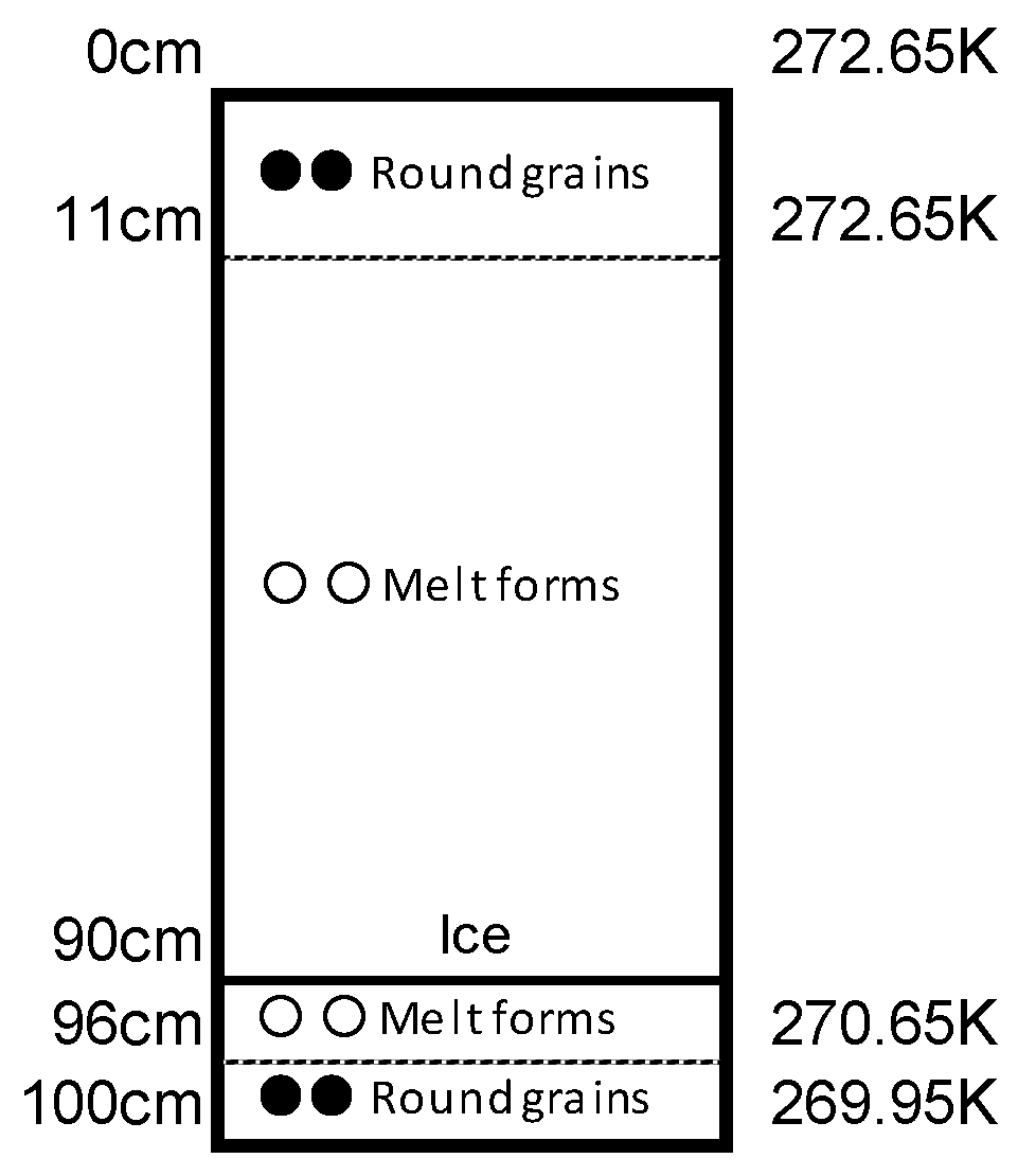
Figure 2, the in situ data for site QH3, as observed by Aoki et al. [
42] on 30 July 2011, includes the stratigraphy, snow classification, and temperature profile, but not snow particle size, snow density, or the snow water content profile. However, snow section observations for the GrIS are very rare and are often the only data available for the GrIS. Therefore, we used stratigraphy, snow classification, and temperature profile on the GrIS as indicators to evaluate snow properties. In the snow section, there is no new snow on the snow surface and “round grains” and “melt forms” are mixed at depths 0 cm to 96 cm. In addition, an ice layer is formed at around 90-cm depth. However, such a detailed vertical local profile cannot be readily related to signals from a satellite with a wide footprint. Thus, the microwave brightness temperatures, calculated using the snow stratigraphy, snow classification, and temperature profile in the RTM, do not necessarily correspond to the satellite microwave brightness temperature averaged over the wide satellite footprint.
In this study, we assumed a range for each physical parameter (emissivity from the ice sheet, layer thickness, snow particle radius, snow density, and snow water content), based on the indicators of stratigraphy, snow classification and temperature profile at the QH3 site. In all cases, we gave these ranges as input in the RTM. We calculated the microwave brightness temperature using the RTM and calculated the cost for each case using a cost function to reflect the correspondence between the satellite and estimated brightness temperatures (Equation (4)), as follows:
where
Tbe18 and
Tbe37 are the estimated brightness temperatures at 18.7 and 36.5 GHz, respectively, and
Tbo19 and
Tbo37 are the AMSR-E brightness temperatures at 18.7 and 36.5 GHz, respectively.
Using this equation, we identified the minimum cost and extracted the corresponding physical parameters for this case. Here, we refer to these values as the optimum physical parameters. Next, we needed to determine the optimum physical parameters (emissivity from ice sheet, layer thickness, snow particle radius, snow density, and snow water content) over the wide satellite footprint, including the QH3 site. As described above, there is no documentation of snow particle radii, snow density, or snow water content profiles at the QH3 site [
42].
In addition, the stratigraphy, snow classification, and temperature profiles at the QH3 site are clearly not valid over the entire region of the wide satellite footprint, which includes the QH3 site. Therefore, we extrapolated a suitable number of snow layers to model this footprint. We assumed the ranges of physical parameters for three and two snow layers, based on the indicators of stratigraphy, snow classification, and temperature profiles at the QH3 site, as described in
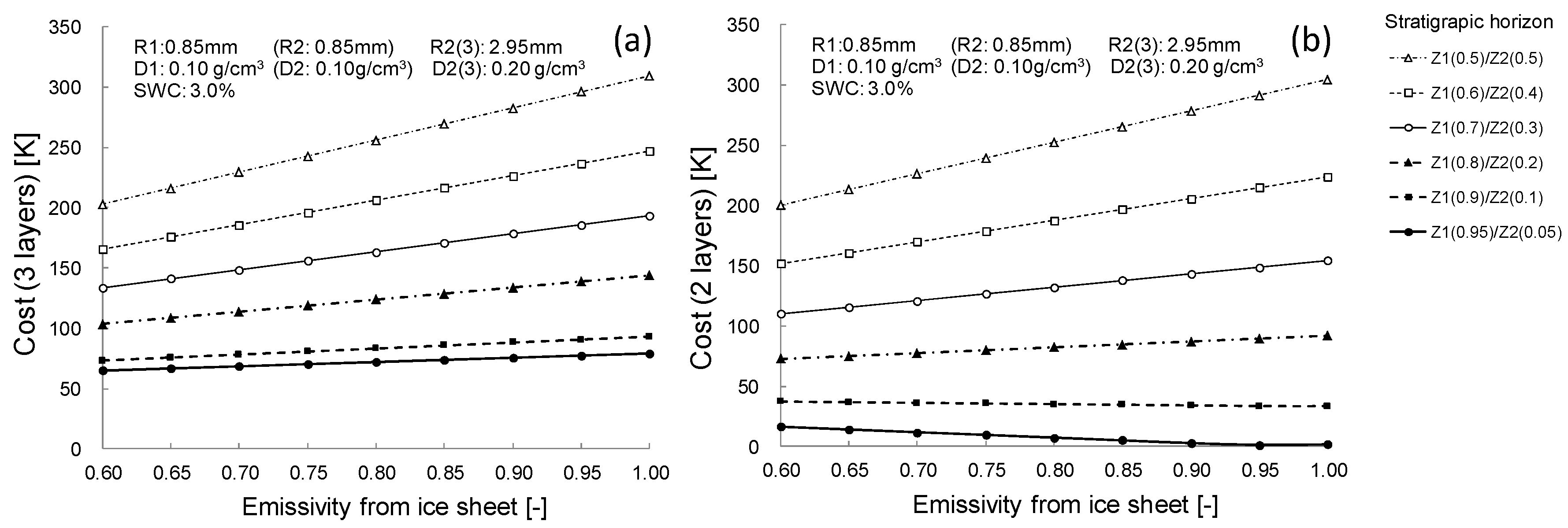
Table 2. Here, we surmised a single snow layer to be too simplistic and unable to describe the actual snowpack, given the snowpack’s extreme heterogeneity over the wide satellite footprint. We conducted tests with two snow layers having upper/bottom layers set to: 0.5 m/0.5 m, 0.6 m/0.4 m, 0.7 m/0.3 m, 0.8 m/0.2 m, 0.9 m/0.1 m, and 0.95 m/0.05 m, giving a total of six cases for a 1.0-m snow depth at the QH3 site. The surface snow layer in the three-snow-layer model had α = 0.01, 0.03, 0.05, 0.08, and 0.10 m, thereby adding five more permutations. We placed the surface layer of the three-snow-layer model on the surface of the uppermost layer in the two-snow-layer model, whereas the bottom layer in the three-snow-layer model is equivalent to the bottom layer in the two-snow-layer model. For example, the two-snow-layer model (0.5 m/0.5 m) corresponds to the three-snow-layer model comprising a surface layer (α m), a middle layer (0.5 m–α m) and a bottom layer (0.5 m). We set all the snow layer thicknesses as input to the RTM. Next, we calculated the microwave brightness temperature using the RTM and the cost for each of the cases using Equation (4) (c.f.
Figure 3).
Figure 3 is based on the optimum physical parameters (snow layer thickness: upper layer = 0.95 m and bottom layer = 0.05 m; snow particle radius: upper layer (R1) = 0.85 mm and bottom layer (R2) = 2.95 mm; snow density: upper layer (D1) = 0.10 g/cm
3 and bottom layer (D2) = 0.25 g/cm
3 and snow moisture (SWC) = 3 vol %), which we determined later. Clearly, the cost for the two-snow-layer model is less than that for three layers. Hence, we concluded that the two-snow-layer model is better at estimating snow depth on the GrIS. Furthermore, we determined that the least cost was associated with the upper (Z1)/bottom layer (Z2) = 0.95/0.05 m.
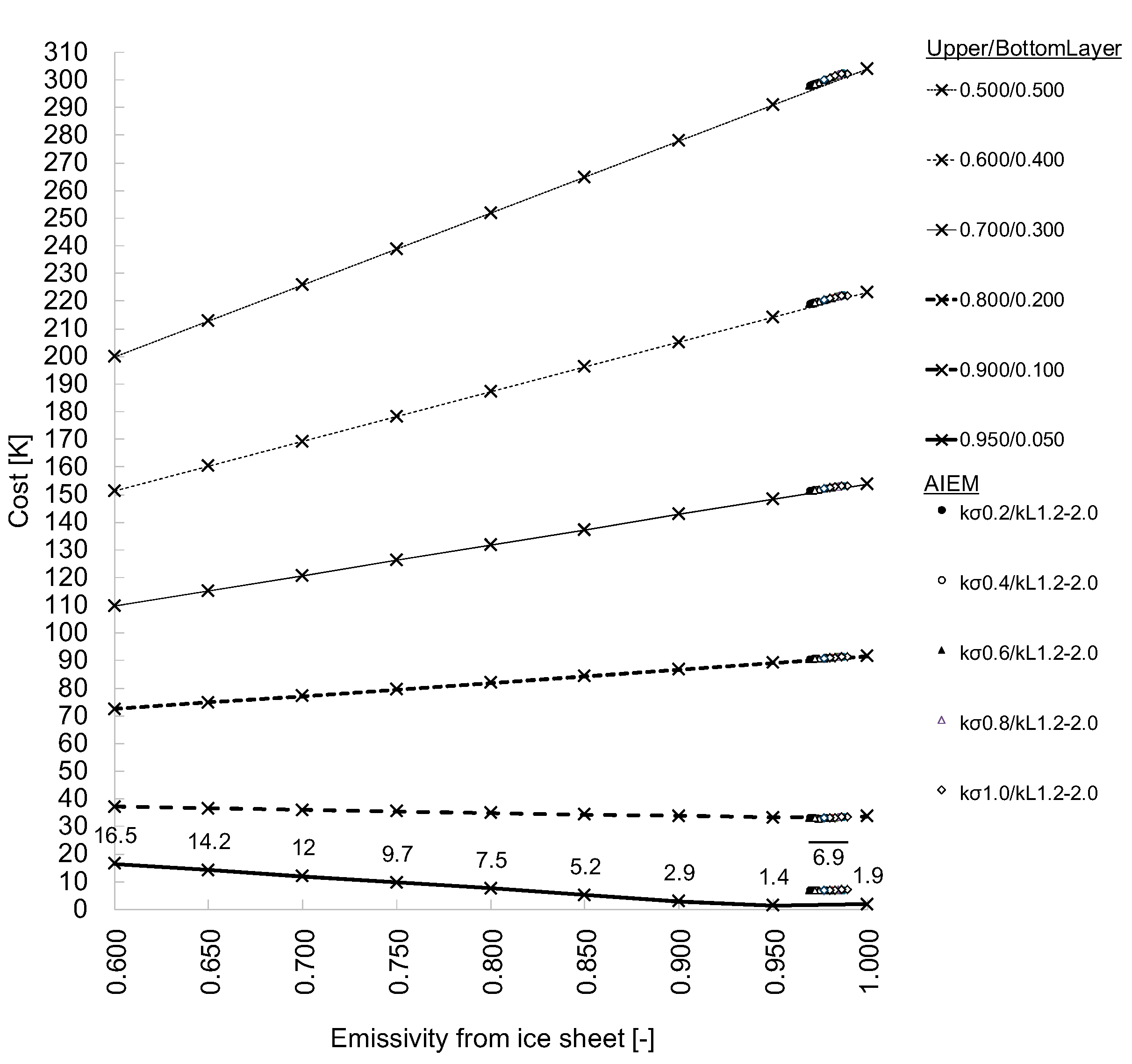
The ice surface of the GrIS is melted by the heat of solar radiation during the summer season, and the surface roughness of the ice sheet is reduced. Therefore, we hypothesized that surface scattering does not take place on the GrIS. However, we performed a test to evaluate this hypothesis, in which the variables in the AIEM are the dielectric constant, the normalized surface root mean square height (kσ), and the correlation length (kL). In this study, we set the dielectric constant for ice (
), but changed the kσ value from 0.2 to 1.0 (in 0.2 intervals), and the kL value from 1.2 to 2.0 (in 0.2 intervals). Then, by varying the kσ and kL values, we explored 25 different cases for each of the six-snow-layer cases having upper/bottom layers of 0.5/0.5 m, 0.6/0.4 m, 0.7/0.3 m, 0.8/0.2 m, 0.9/0.1 m, and 0.95/0.05 m. In addition, we varied the emissivity of the ice sheet from 0.6 to 1.0 in 0.05 intervals, and input these values into the RTM. We then calculated the microwave brightness temperature using the RTM, and the cost for each case using Equation (4) (c.f.
Figure 4). To clearly illustrate our results,
Figure 4 is based on the optimum physical parameters (snow particle radius: upper layer (R1) = 0.85 mm and bottom layer (R2) = 2.95 mm, snow density: upper layer (D1) = 0.10 g/cm
3 and bottom layer (D2) = 0.25 g/cm
3, and snow moisture (SWC) = 3 vol %), which we determined later. Clearly, the cost of the upper/bottom layer = 0.95/0.05 m is lowest. Likewise, the lowest cost of 1.4 was associated with an emissivity of 0.95. This also yields a value smaller than the average cost of the 25 cases (
) of the AIEM. In the RTM, we calculated the microwave radiation related to volume scattering by the background particles under the snowpack and are transferred from the bottom to the top layer. Next, we used the AIEM to determine the surface scattering and calculated the emissivity from the background surface. Thus, the only information required from under the snowpack is the emissivity from the background surface. We can also evaluate the volume scattering in the background when the background is a dense medium composed of many particles. However, our RTM cannot evaluate the volume scattering in the ice sheet because the ice sheet is a continuous block of ice. Hence, as the emissivity from the ice sheet, we assumed values in a range from 0.6 to 1.0 in 0.05 intervals after the microwave radiation was transferred to the ice sheet, and input these values into the RTM. Simultaneously, we varied other variables (kσ from 0.2 to 1.0 in 0.2 intervals, and kL from 1.2 to 2.0 in 0.2 intervals) of the AIEM and input them into the RTM. Next, we calculated the costs for all cases using the microwave brightness temperature, as calculated from the RTM. Lastly, we extracted the minimum cost and its corresponding conditions. In consequence, we found the optimum condition over the wide satellite footprint covering the QH3 site to be a two-layer snow structure, with a 0.95-m upper layer and a 0.05-m bottom layer snow thickness, and an emissivity value of 0.95 from the ice sheet.
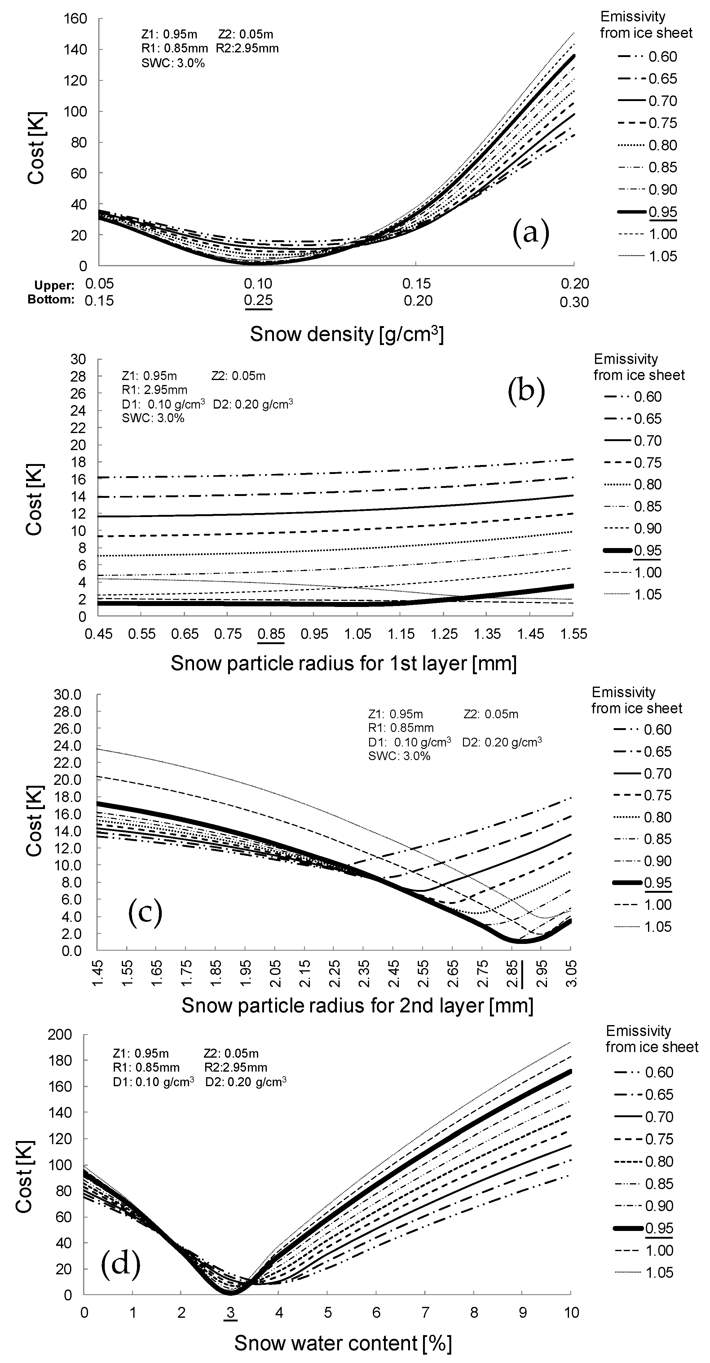
With two layers as the snow layer structure, with a 0.95-m upper layer/0.05-m bottom layer snow thickness, and 0.95 emissivity from the ice sheet, we set all variations of snow particle radius, snow density, and snow water content according to the variability range in
Table 2(2). Next, we calculated the microwave brightness temperature using the RTM and evaluated the cost for each case using Equation (4) (
Figure 5). Clearly, the cost reduces when the snow densities are 0.10/0.25 g/cm
3, the snow particle radii are 0.85/2.95 mm in the upper/bottom layers, and the snow water content is 3 vol %. Therefore, we used these values as the optimum snow densities, snow particle radii, and snow water contents over the wide satellite footprint covering the QH3 site.
For our initial guesses for this study, we applied the optimum physical parameters shown in
Table 3 (emissivity from the ice sheet of 0.95, upper snow layer thickness of 0.95 m, bottom snow layer thickness of 0.05 m, snow density in upper snow layer of 0.10 g/cm
3, snow density in bottom snow layer of 0.25 g/cm
3, snow particle radius in upper snow layer of 0.85 mm, snow particle radius in bottom snow layer of 2.95 mm, and snow water content of 3 vol %) over the wide satellite footprint including the QH3 site. To obtain various cases for these initial guesses, as indicators, we used the parameter ranges listed in
Table 3, based on the optimum physical parameters over the wide satellite footprint covering the QH3 site. When assuming these ranges, we also considered that although the wide satellite footprint covering the QH3 site is located on the northwest coast of the GrIS, their variability ranges should apply to the entire GrIS. Although the QH3 site was observed on 30 July 2011, the period of interest covers the end of the midwinter season to the snowmelt season. Ideally, we should evaluate the emissivity from the ice sheet and the RTM performance for the ice surface scattering using the deep snow observation site of López Moreno et al. [
44]. However, the observation data for this site did not include the stratigraphy, snow classification, or a temperature profile. Therefore, to estimate snow depth over the entire GrIS, we used the optimum emissivity from the ice sheet over the wide satellite footprint covering the QH3 site. In our results (
Section 5), we discuss the validity of using the 0.95 emissivity value to estimate snow depth.
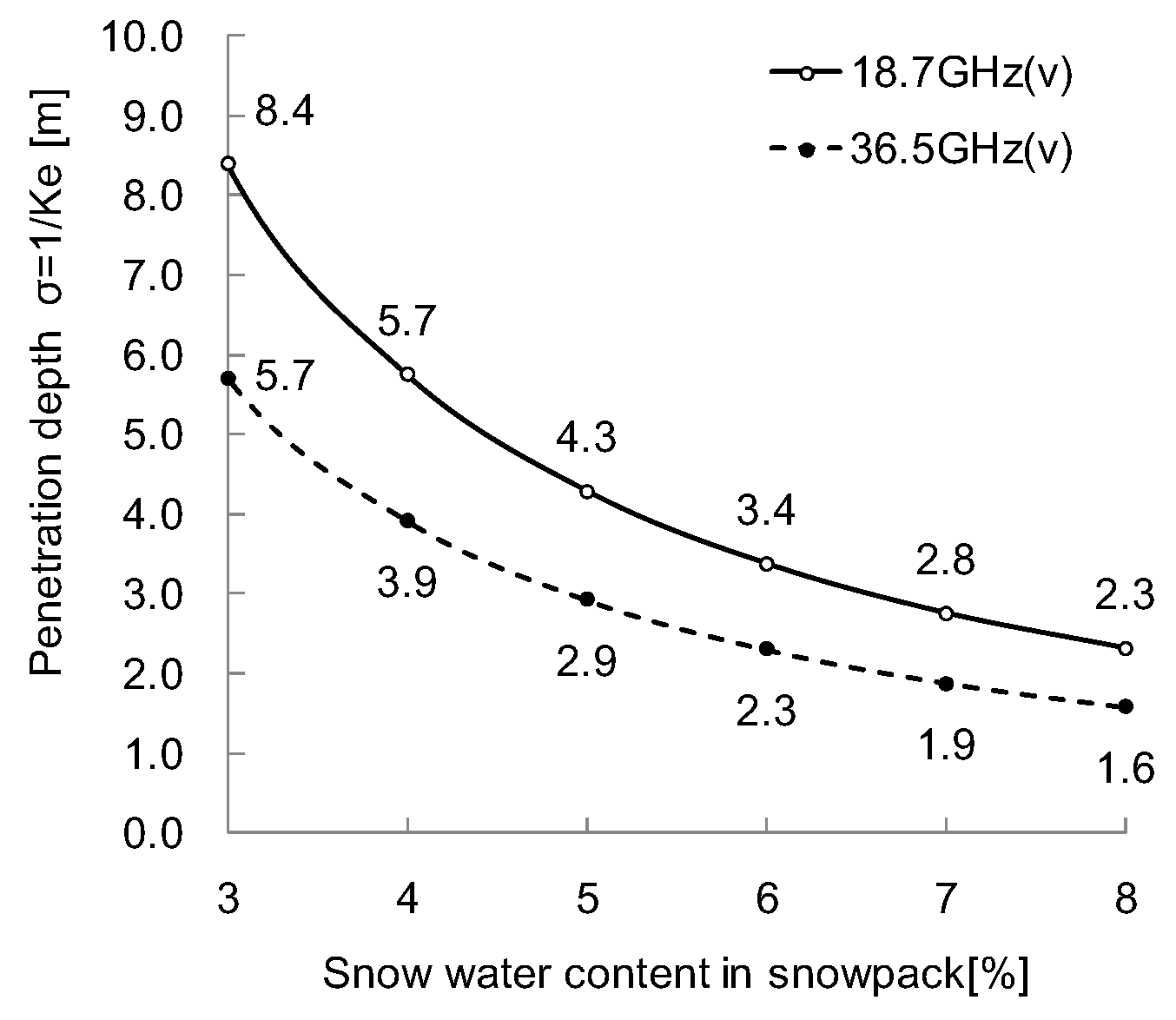
Figure 6 shows the penetration depths for 18.7 and 36.5 GHz (v), based on the extinction coefficient (Ke) of the snowpack calculated by the RTM. Clearly, the penetration depth decreases with an increase in the snow water content in the snowpack. When the snow water content is less than 4 vol %, the penetration depth of 36.5 GHz is greater than 2 m. The penetration depth of 36.5 GHz is less than 2 m, however, when the snow water content is greater than 6 vol %. Thus, there is a limit to the RTM’s snow estimation capability in snow depths from 2–3 m.
In this study, we varied the snow surface temperature, snow layer thickness, snow density, snow particle radius, and snow water content across the ranges given in
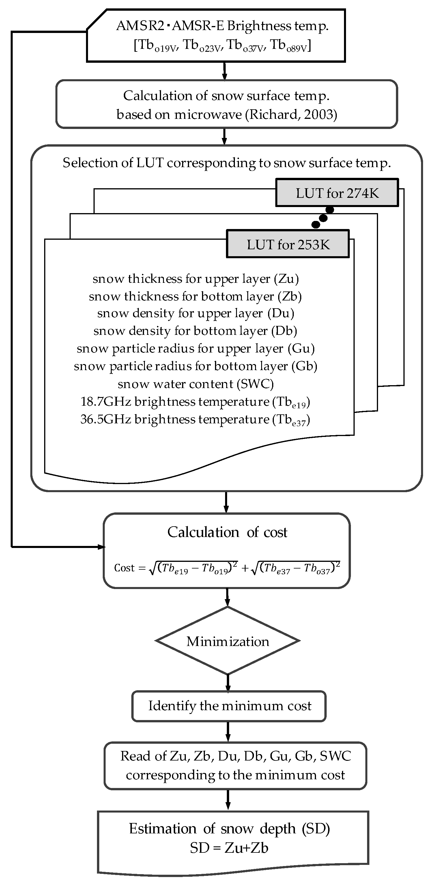
Table 3 and input these values into the RTM. We then calculated the microwave brightness temperature for frequencies of 18.7 and 36.5 GHz (v). We created a lookup table (LUT) for all snow thickness cases for the upper and bottom layers, snow densities for the upper and bottom snow layers, snow particle radii for the upper and bottom layers, and snow water contents, for the 18.7- and 36.5-GHz microwave brightness temperatures. We also created a LUT for each snow surface temperature from 253–274 K, at one K intervals. Thus, we generated a total of 22 LUTs. Using these LUTs, we then developed a simple snow retrieval algorithm (
Figure 7) that has the following flow path. We input the AMSR-E (or AMSR2) brightness temperatures for 18.7, 23.8, 36.5, and 89.0 GHz (
Tbo19,
Tbo23,
Tbo37, and
Tbo89) into the algorithm and calculate the snow surface temperature using the experimental formula developed by Richard et al. [
45]. We then select a LUT corresponding to the calculated snow surface temperature for microwave brightness temperatures of 18.7 and 36.5 GHz (
Tbe19 and
Tbe37) for all cases in the LUT, and calculate the cost using Equation (4). Next, we extract the minimum cost from all cases and output the optimum snow thickness for the upper and bottom layers, snow densities for the upper and bottom layers, snow particle radii for the upper and bottom layers, and snow water content corresponding to the minimum cost. Lastly, we estimate the snow depth (=snow thickness for upper + bottom layers).
5. Results
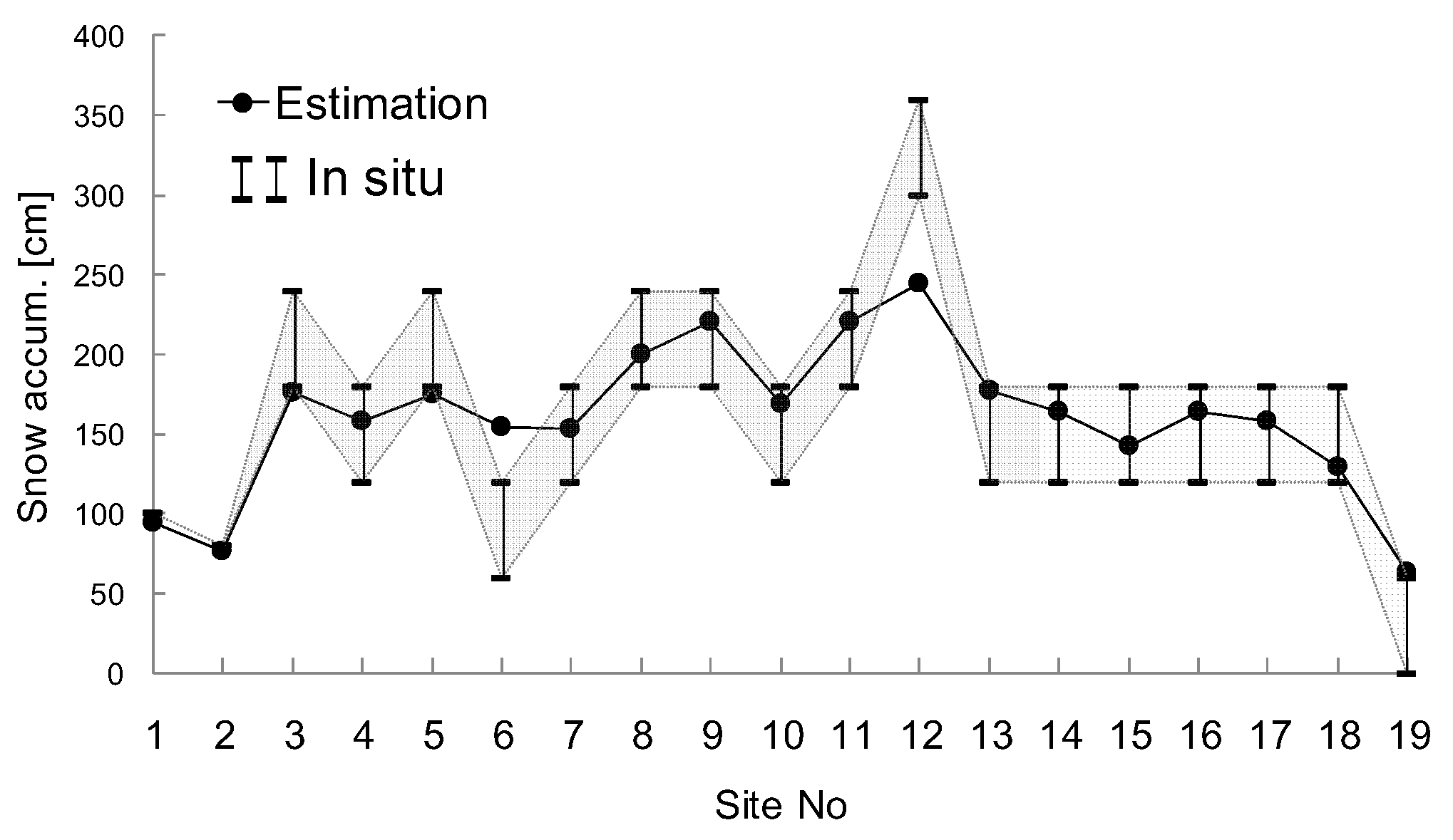
Figure 8 compares the estimated and in situ snow depths at 19 sites in Greenland, the locations of which are shown in
Figure 1. The estimated snow depths fit the in situ snow depths recorded at sites 1 and 2, and are in relatively good agreement with the in situ snow depths at sites 3 to 19. However, we recognize that microwave remote sensing cannot estimate dramatic spatial changes in snow depths as in the cases of sites 6 and 12, because the satellite footprint is too wide. We used an optimum emissivity value of 0.95 for the entire GrIS to generate the results shown in
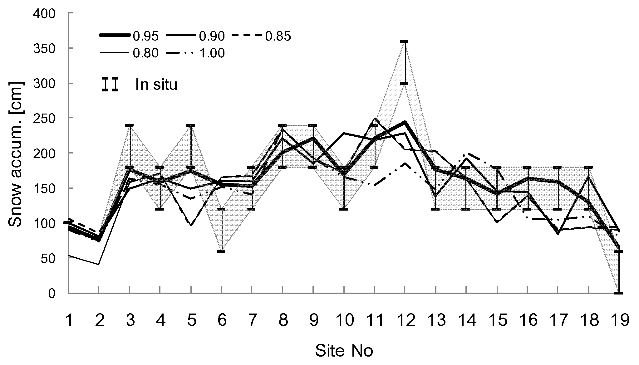
Figure 8. However, the inaccuracy in the emissivity values across the GrIS may generate discrepancies, as seen at sites 6 and 12. We calculated LUTs for emissivity values of 0.80, 0.85, 0.90, 0.95, and 1.00, and estimated snow depth based on these LUTs (
Figure 9). We then calculated the RMSE ratios to evaluate these results (
Table 4). We calculated the RMSE values for the in situ versus estimated snow depths at each emissivity and compared the RMSEs for emissivity values of 0.80, 0.85, 0.90, and 1.00 with the RMSE value for a 0.95 emissivity. Here, we define this ratio as the RMSE ratio. Given the spatial heterogeneity in snow depth, we used mean depth as the in situ snow depth at sites 3 to 19. As shown in
Figure 9 and
Table 4, we found no improvement in estimated snow depth using LUTs for emissivity values of 0.80, 0.85, 0.90, and 1.00. Hence, we affirm the reliability of the optimum emissivity (0.95) used to estimate snow depth over the GrIS.
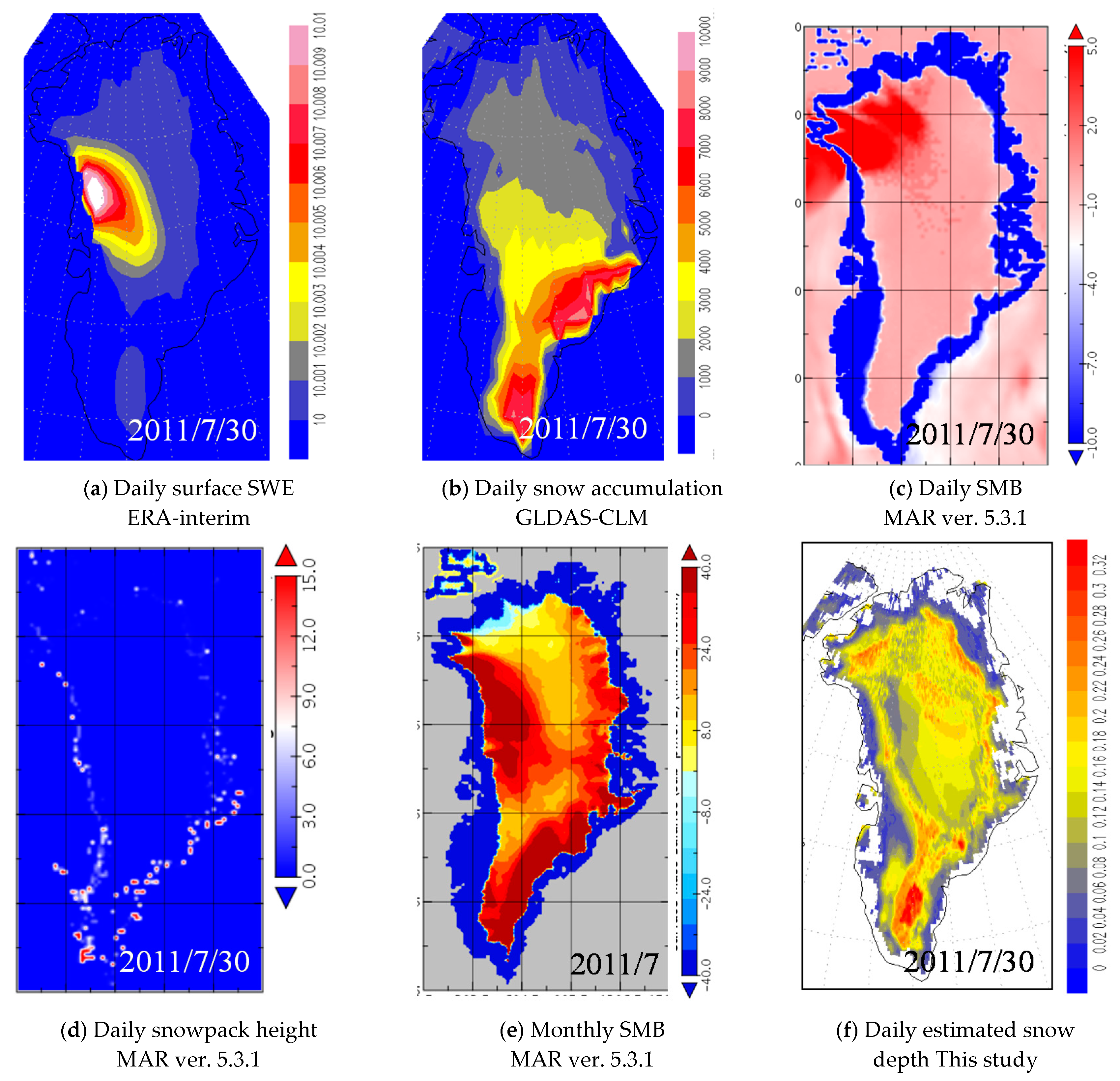
Figure 10,
Figure 11 and
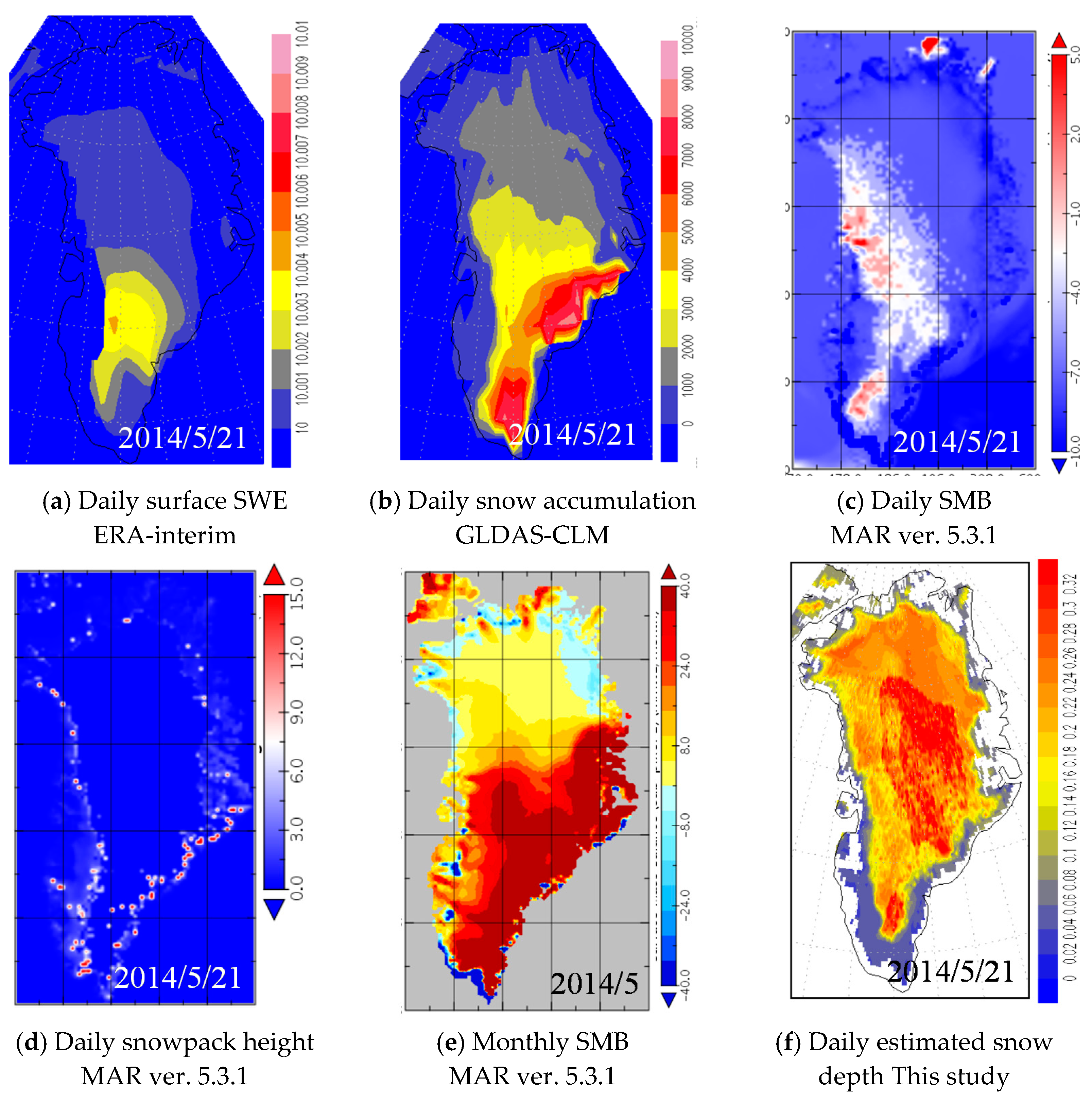
Figure 12 show the spatial distributions on the respective dates of 30 July 2011; 21 May 2014; and 11 June 2014 for the following variables: (a) the daily surface snow water equivalent (SWE; m) from the ERA-interim, with 0.75° spatial resolution; (b) the daily surface accumulation of snow (kg/m
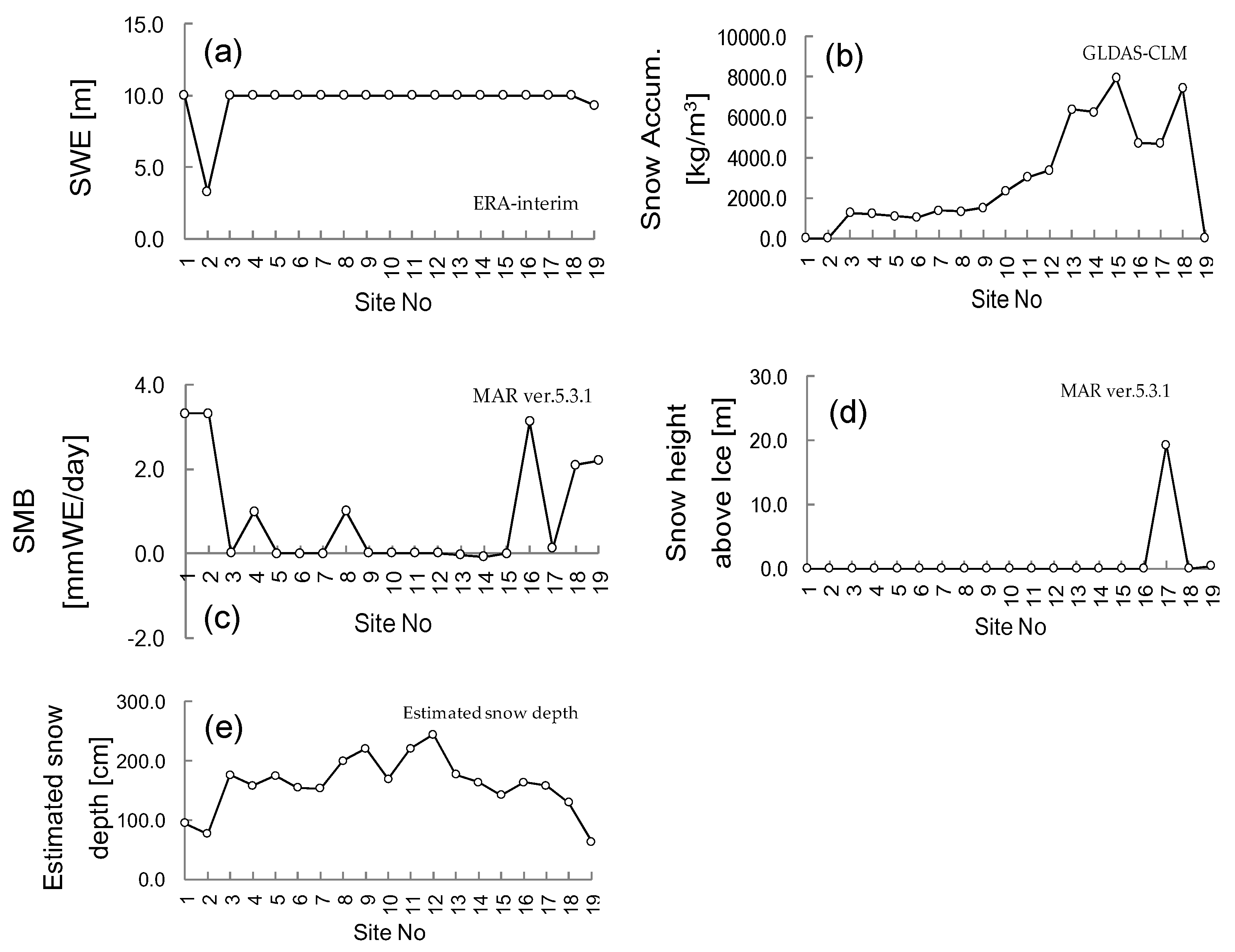
2) from the GLDAS-CLM, with 1° spatial resolution; (c) the daily surface mass balance (SMB; mm WE/day) from MAR ver. 5.3.1, based on the NCEPv1; (d) the snowpack height above ice (m) from MAR ver. 5.3.1 based on the NCEPv1, with 0.2° spatial resolution; (e) the monthly surface mass balance (SMB; mm WE/month) from MAR ver. 5.3.1 20CRv2c; and (f) the distribution of the estimated snow depth (cm) from this study, with a 0.25° spatial resolution. As a reference,
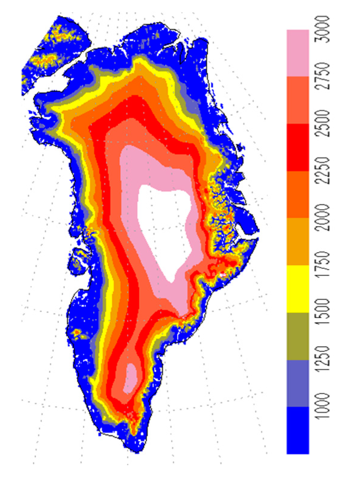
Figure 13 shows Greenland elevations derived from the NOAA elevation product.
Figure 14a–d,f shows the output at the 19 sites corresponding to the values given in
Table 1.
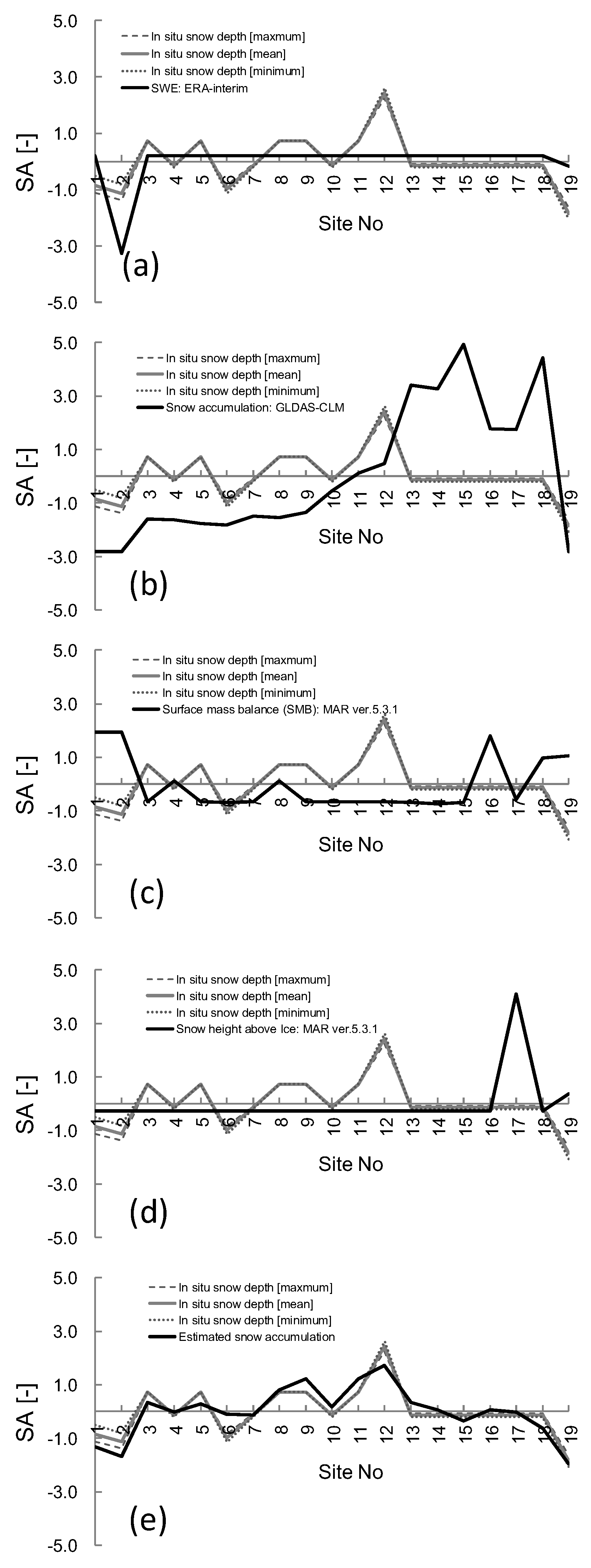
Various properties are reflected in the spatial distributions of each product; therefore, identifying the correct spatial distribution for seasonal snow depth from these products is difficult. In an integrated view, there is a common pattern to the spatial distributions of SWE from ERA-interim, and daily SMB from MAR on the 21 May 2014. Likewise, snow depth from GLDAS-CLM, and monthly SMB from MAR show a positive association in the southeast high-elevation mountain region. They also have a similar spatial distribution to the snow depths estimated in this study. Estimated snow depth in the central region of the GrIS is relatively higher than in other regions. However, we believe our estimated snow depth to be reasonable, because the central region has an elevation of 2500 m or more. However, we cannot check the actual snow depth in this region, so we have no choice but to validate the estimation accuracy using in situ snow depth data.
Each product has a different unit and definition, as described in
Figure 10,
Figure 11 and
Figure 12 and
Figure 14, and therefore cannot be directly compared. Instead, we investigated the standardized anomaly (SA) index of each product. First, we determined the best-fit distribution pattern that minimized the corrected Akaike information criterion (Equation (5)); Akaike [
46]) and Bayesian information criterion (Equation (6)) for the main output parameter of each product, using maximum likelihood estimates. Next, we used Equation (7) to transform these best-fit distributions into normal distributions. In addition, we standardized all the values by dividing the anomaly by the standard deviation of the transformed parameter which corresponds to using Equation (8) to calculate the standardized anomalies of the transformed parameters.
Table 5 shows the determined best-fit distribution pattern for the main output parameter of each product.
Figure 15 shows our validation, based on the SA index for each product, and
Table 6 lists our accuracy values (RMSE, bias, and correlation coefficient).
Figure 15e shows the potential of our method for estimating snow depth.
where
,
,
, and
is the distribution function for any parameter
x.
7. Conclusions
In this study, we used the RTM at a typical site (QH3 site), as observed by Aoki et al. [
42], to investigate the microwave properties of seasonal snow depth on the GrIS, and we determined the optimum physical parameters (emissivity from the ice sheet, snow density, snow particle size, and snow water content).
In this study, we investigated the microwave properties of seasonal snow depth on the GrIS using the RTM at a typical site (QH3 site), observed by Aoki et al. [
42], and determined optimum physical parameters (emissivity from ice sheet, snow density, snow particle size, and snow water content). To evaluate seasonal snow depth over the entire GrIS from the end of the midwinter season to the snowmelt season, we set the variability range based on these optimum physical parameters at the typical site (QH3 site), and calculated LUTs for the microwave brightness temperatures. To estimate seasonal snow depth on the GrIS solely from satellite microwave brightness temperature, we developed a simple snow retrieval algorithm using these LUTs, and estimated seasonal snow depth over the entire GrIS. Although we found that microwave remote sensing could not estimate a dramatic spatial change in snow depth, our estimated snow depths had relatively good overall agreement with the in situ snow depths at the 19 sites observed by Aoki et al. [
42] and López Moreno et al. [
44]. Next, we compared the spatial distribution of the estimated snow depths over the entire GrIS was those of other major products: SWE from ERA-interim, snow accumulation from GLDAS-CLM, and SMB and the snow height above ice from MAR ver. 5.3.1. As a characteristic tendency over the GrIS, we derived the deep snow distribution in the southeast high-elevation region similar to the snow accumulation of the GLDAS-CLM and the monthly SMB of MAR ver. 5.3.1. Subsequently, we evaluated the accuracies of our estimated snow depths and those of the other products using the SA index at the 19 sites. The calculated accuracies of our estimated snow depth were 0.43, 0.00, and 0.89 for the RMSE, bias, and correlation coefficient (r), respectively, although the accuracy of the other products was 0.95 to 0.43, −0.91 to −6.07 and −0.11 to −0.35, respectively. Thus, we demonstrated the applicability of our satellite snow depth retrieval algorithm based on our RTM. However, we acknowledge the following limitations. Our algorithm in this study targeted the end of the midwinter season to the snowmelt season on the GrIS. In addition, the reliability of our algorithm decreases for locally deep snow depths because our RTM has the limitation of reduced microwave penetration at the depths of 2–3 m. The reliability of our algorithm decreases for locally shallow snow depths because our RTM cannot estimate such snow depths using the spatially averaged microwave brightness temperature in the wide footprints of AMSR-E and AMSR2. Furthermore, we consider that to estimate snow depth with great accuracy using microwave remote sensing, we must rely on the following method: (1) Calculate the variation of the physical parameters (snow grain growth and aging of snow density) using the land surface model from the beginning of snow accumulation and, as initial guesses, estimate the snow thickness, snow particle radius, snow density, and snow water content. Next, use these initial guesses as input into the RTM and calculate the microwave brightness temperature. (2) Use a cost function to calculate cost that reflects the correspondence of the simulated and satellite microwave brightness temperatures. Determine the minimum cost extracted using the assimilation scheme and estimate the snow depth corresponding to the minimum cost conditions. However, we consider that the optimum snow depth cannot be estimated by this process alone. (3) To estimate the optimum snow depth, we should generate various cases around the initial guesses values using a perturbation method (e.g., a genetic particle filter; Qin et al. [
47]), and then implement step (2) for all cases. In this way, we can obtain an optimum snow depth corresponding to the minimum cost. We believe it is necessary to introduce this perturbation process to estimate the optimum snow depth. Here, we assumed that the initial guesses were the set of optimum physical parameters for the wide satellite footprint covering the QH3 site. We conclude that the cost related to the emissivity from the ice sheet is lower than that based on the AIEM to evaluate surface scattering. Ideally, we should evaluate the emissivity of the ice sheet using the deep snow region studied by López Moreno et al. [
44], but these observations lack stratigraphy, snow classification, and a temperature profile data. Therefore, to estimate snow depth over the entire GrIS, we used the optimum emissivity of 0.95 from the ice sheet over the wide satellite footprint covering the QH3 site. We validated the applicability of a 0.95 emissivity for snow depth estimation and confirmed its reliability against other measures. In conclusion, we demonstrated the potential for estimating seasonal snow depth using only passive microwave remote sensing on the GrIS during snow melting and an emissivity of 0.95 for the entire GrIS.
Furthermore, we affirmed the possibility of performing step (3) in the above method. In the future, we plan to acquire better spatiotemporal snow observation data, including snow section data. We are also developing a data assimilation system comprising steps (1) to (3), and will continue to investigate the effects of surface scattering on the ice sheet.


