Article

Multispectral LiDAR Point Cloud Classification: A Two-Step Approach

1
State Key Laboratory of Information Engineering in Surveying, Mapping and Remote Sensing, Wuhan University, 129 Luoyu Road, Wuhan 430072, China
2
Collaborative Innovation Center of Geospatial Technology, 129 Luoyu Road, Wuhan 430072, China
3
Institute of Spacecraft System Engineering, China Academy of Space Technology, Beijing 100094, China
4
School of Physics and Technology, Wuhan University, 129 Luoyu Road, Wuhan 430072, China
5
State Key Laboratory of Magnetic Resonance and Atomic and Molecular Physics, Wuhan Institute of Physics and Mathematics, Chinese Academy of Sciences, 30 Xiao Hongshan Road, Wuhan 430072, China
*
Authors to whom correspondence should be addressed.
Remote Sens. 2017, 9(4), 373; https://doi.org/10.3390/rs9040373
Submission received: 20 September 2016 / Revised: 7 April 2017 / Accepted: 13 April 2017 / Published: 17 April 2017

Abstract

:
Target classification techniques using spectral imagery and light detection and ranging (LiDAR) are widely used in many disciplines. However, none of the existing methods can directly capture spectral and 3D spatial information simultaneously. Multispectral LiDAR was proposed to solve this problem as its data combines spectral and 3D spatial information. Point-based classification experiments have been conducted with the use of multispectral LiDAR; however, the low signal to noise ratio creates salt and pepper noise in the spectral-only classification, thus lowering overall classification accuracy. In our study, a two-step classification approach is proposed to eliminate this noise during target classification: routine classification based on spectral information using spectral reflectance or a vegetation index, followed by neighborhood spatial reclassification. In an experiment, a point cloud was first classified with a routine classifier using spectral information and then reclassified with the k-nearest neighbors (k-NN) algorithm using neighborhood spatial information. Next, a vegetation index (VI) was introduced for the classification of healthy and withered leaves. Experimental results show that our proposed two-step classification method is feasible if the first spectral classification accuracy is reasonable. After the reclassification based on the k-NN algorithm was combined with neighborhood spatial information, accuracies increased by 1.50–11.06%. Regarding identification of withered leaves, VI performed much better than raw spectral reflectance, with producer accuracy increasing from 23.272% to 70.507%.

Graphical Abstract

1. Introduction

Target classification techniques based on remotely sensed data are widely used in many disciplines such as resource exploration, outcrop geology, urban environmental management, and agriculture and forestry management [1,2,3,4,5,6,7,8,9,10,11]. Target classification enables a more accurate understanding of targets and therefore supports better decision-making. Thus, the remote sensing community has been studying classification techniques and methods for many years. Target classification techniques and methods have matured and become diverse, given the recent advances in remote sensing technology and pattern recognition, newer approaches have extended and built upon traditional technologies.
Before multispectral LiDAR, two major technologies provided data for target classification, spectral imaging and light detection and ranging (LiDAR). Multispectral LiDAR data have similarities to both spectral imaging and LiDAR, thus the classification methods based on spectral images, and LiDAR data have acted as a reference when multispectral LiDAR techniques were initially developed. Support vector machine (SVM) is a supervised [12] classification method, and a popular non-parametric classifier widely used in the machine learning and remote sensing communities [13,14,15]. SVM can effectively overcome the curse of dimensionality and overfitting [16,17,18]. With the help of SVM, spectral image classification has performed successfully in many experiments [19,20]. Compared to spectral images, the classification of LiDAR point clouds is less mature because LiDAR requires complicated data processing and its wide application emerged only recently. LiDAR classification experiments have been conducted for applications in urban building extraction and forest management [21,22,23]. Spectral imaging and LiDAR have demonstrated their effectiveness for target classification; however, spectral imaging lacks three-dimensional (3D) spatial information, and conventional LiDAR systems operate on a single wavelength, which lacks spectra for objects.
Classification experiments employing complementary information from both LiDAR and images were conducted. The performance of classification generally were improved with the complementary information. Guo et al. [24] selected the random forests algorithm as a classifier and used margin theory as a confidence measure of the classifier to confirm the relevance of input features for urban classification. The quantitative results confirmed the importance of the joint use of optical multispectral and LiDAR data. García et al. [25] presented a method for mapping fuel types using LiDAR and multispectral data. Spectral intensity, the mean height of LiDAR returns and the vertical distribution of fuels were used with an SVM classification combining LiDAR and multispectral data. Laible et al. [26] conducted an object-based terrain classification with random forests by extracting 3D LIDAR-based and camera-based features. The 3D LIDAR-based features included maximum height, the standard deviation of height, distance, and the number of points. The results showed that classification based on extracted features from camera and LiDAR was feasible under different lighting conditions. The complementary information of LiDAR and images, however, can only be used effectively after accurate registration, which involves many difficulties [27].
As a novel remote sensing technology, multispectral LiDAR can capture both spectral and spatial information simultaneously [28,29], and has been used in various fields [30,31,32,33]. The introduction of the first commercial airborne multispectral LiDAR, Optech Titan, made multispectral LiDAR land cover classification feasible. Wichmann et al. [34] conducted an exploratory analysis of airborne-collected multispectral LiDAR data with a focus on classifying specific spectral signatures by using spectral patterns, thereby showing that a flight dataset is suitable for conventional spatial classification and mapping procedures. Zou et al. [35] presented an Object Based Image Analysis (OBIA) approach, which only used multispectral LiDAR point clouds datasets for 3D land cover classification. The results show that an overall accuracy of over 90% can be achieved for 3D land cover classification. Ahokas et al. [36] suggested that intensity-related and waveform-type features can be combined with point height metrics for forest attribute derivation in area-based prediction, and currently is an operatively applied forest inventory process used in Scandinavia. The airborne multispectral LiDAR Optech Titan system shows promising potential for land cover classification; however, as Optech Titan acquires LiDAR points in three channels at different angles, points from different channels do not coincide at the same GPS time [34]. Therefore, data processing involves finding corresponding points, which is a disadvantage of Optech Titan data.
Terrestrial multispectral LiDAR however, can overcome this disadvantage, and classification attempts have been undertaken. Hartzell et al. [37] classified rock types using the data from three different commercial terrestrial laser scanning systems with different wavelengths and compared the results with passive visible wavelength imagery. This analysis indicated that rock types could be successfully identified with radiometrically calibrated multispectral terrestrial laser scanning (TLS) data, with enhanced classification performance when fused with passive visible imagery. Gong et al. [38] compared the performance of different detection systems finding that classification based on multispectral LiDAR was more accurate than single-wavelength LiDAR and multispectral imaging. Vauhkonen et al. [39] studied the classification of spruce and pine species using multispectral LiDAR data with linear discriminant analysis. They found that the accuracies of two spectrally similar species could be improved by simultaneously analyzing reflectance values and pulse penetration. There are two kinds of classification for point clouds: object-based classification and point-based classification [40,41]. Object-based classification is for objects, which are composed of many points while point-based classification is for individual points. Most of the aforementioned classification experiments were point-based, based on statistical models and image analysis; but have not yet employed neighborhood spatial information to improve and enhance classification results.
The classification results could be improved considering the low signal to noise ratio of this kind of novel sensor data. Moreover, the reasons of low signal to noise ratio could be: high noise in the reflection signal collection [42,43], the close range experimental setup that caused high sensitivity of the sensing process [44], the instability of the laser power and the multi-return of the LiDAR beam [45]. The low signal to noise ratio brings about instability in the spectral intensity value of points, creating salt and pepper noise in the spectral-only classification [38] and thus lowering overall classification accuracy. To solve this problem, we proposed a subsequent k-nearest neighbors (k-NN) clustering step using neighborhood spatial information with a better classification outcome, overall.
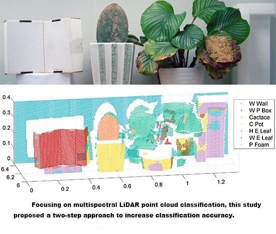
This article proposes a two-step approach for point-based multispectral LiDAR point cloud classification. First, we classified a point cloud based on spectral information (spectral reflectance or vegetation index). Second, we reclassified the point cloud using neighborhood spatial information. In the first step, the vegetation index (VI) was introduced into the classification of healthy and withered leaves. In the second step, the k-NN algorithm was employed with neighborhood spatial information for reclassification. The feasibility of the two-step classification method and the efficiency of neighborhood spatial information for increasing classification accuracy were assessed.

2. Materials

2.1. Equipment

The equipment used in this experiment was the multi-wavelength canopy LiDAR (MWCL) designed and established by Gong [28]. The MWCL system consists of three subsystems: the laser source, the optical receiver assembly, and the data acquisition and processing system. The laser sources are four independent semiconductor laser diodes with four wavelengths: 556, 670, 700, and 780 nm. The laser lights are synthesized into one beam and then transmitted to the target. Backscattered radiation is received by the optical receiver assembly, this equipment includes an achromatic Schmidt–Cassegrain telescope with a diameter of 20 cm and four photon-counting detectors. The platform details of the MWCL are described in a study published by Gong [28]. Using the MWCL system, multispectral LiDAR point cloud data were acquired.

2.2. Materials and Data

This research was conducted at the laboratory at Wuhan University in Central China. Seven experimental materials were used: a white wall; a white paper box; a cactus; a ceramic flowerpot; healthy scindapsus leaves; withered scindapsus leaves; and plastic foam. These seven materials were selected for two reasons: first, the artificial and vegetable materials were to demonstrate the multispectral LiDAR’s ability to classify artificial and vegetable targets; and second, the healthy and withered scindapsus leaves were included to validate whether different growing states could be recognized correctly.
The experimental materials were in decimeter scale and placed at a horizontal distance of six to six and a half meters from the MWCL receiver. The materials were lined up in front of a white wall. The height and length of the point cloud was 0.41 and 1.39 m. A photo and a MWCL point cloud of the experimental scene are shown in Figure 1 and Figure 2.
The MWCL data had seven dimensions, with four channels for spectra and three dimensions of spatial position (X,Y,Z), that is, the multispectral LiDAR point cloud. This data contained more information than either the spectral image or conventional LiDAR point cloud alone. The spectral image possesses abundant spectral information but only two-dimensional planar spatial information. The point cloud from one kind of conventional LiDAR, without an optical camera, possesses only one channel of spectrum and three-dimensional spatial positional information. The multispectral LiDAR point cloud combines the advantages of a spectral image and a conventional LiDAR point cloud.

2.3. Variation of Raw Spectral Reflectance

There were seven targets in the laboratory, each of which had a different spectral reflectance. The realistic spectral reflectance of the same target also varies from point to point because the realistic spectral reflectance is influenced by the spectral properties of a target, the incidence angle, transmission distance, and atmospheric attenuation.
The spectral properties of a target is the main factor in spectral reflectance, and is also the fundamental information on which the classification can be based. Given the variance of the surface of targets, the incidence angle of the beam changed for all targets, especially vegetation. Transmission distance was already considered when calibrating the echo reflectance, based on the radar equation. Atmospheric attenuation was not considered in this experiment because the transmission distance was too short (approximately 6–6.5 m), and the experiment was conducted in a clean room. The variation of raw spectral reflectance on seven targets is shown in Figure 3.
Figure 3 shows that the white wall maintained a high reflectance at all four wavelengths; most reflectances were between 0.9 and 1.0. The white paper box had a high reflectance at the other three wavelengths except for 670 nm (approximately 0.3–0.4). The cactus had a low reflectance (0.1–0.4) at three wavelengths except at 780 nm. The reflectance of the ceramic flowerpot was moderate (0.3–0.6) but was high at 700 nm. Healthy and withered scindapsus leaves had a similar reflectance at three wavelengths except at 700 nm. The reflectance of withered leaves at 700 nm was visibly higher than that of healthy leaves. Thus, 700 nm is a significant wavelength to distinguish between healthy and withered scindapsus leaves. The plastic foam exhibited great reflectance fluctuations over three wavelengths apart from 700 nm (nearly one), which means that the spectral feature of plastic foam was unstable. However, other targets had a steady spectral reflectance. This result serves as the basis of the classification based on spectral information.

3. Methods

The classification process consisted of two steps: routine classification based on spectral information followed by spatial majority k-NN clustering. First, we classified the multispectral LiDAR point cloud with an SVM classifier using spectral information (raw spectral reflectance and VI). Second, the k-NN algorithm was used by neighborhood spatial information to reclassify the multispectral LiDAR point cloud based on the first step. The details are described in the following sections.
In the first step, the classification experiments using raw spectral reflectance value included: (1) seven individual targets; (2) artificial and vegetable targets; and (3) healthy and withered scindapsus leaves. The classification based on VI included: (1) artificial and vegetable targets; and (2) healthy and withered scindapsus leaves. In the second step, all the aforementioned classification experiments were reclassified using neighborhood spatial information with the k-NN algorithm.

3.1. Classification Based on Raw Spectral Reflectance

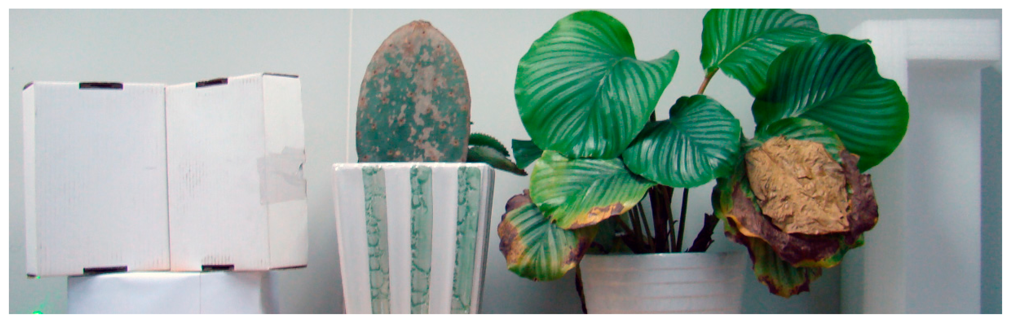
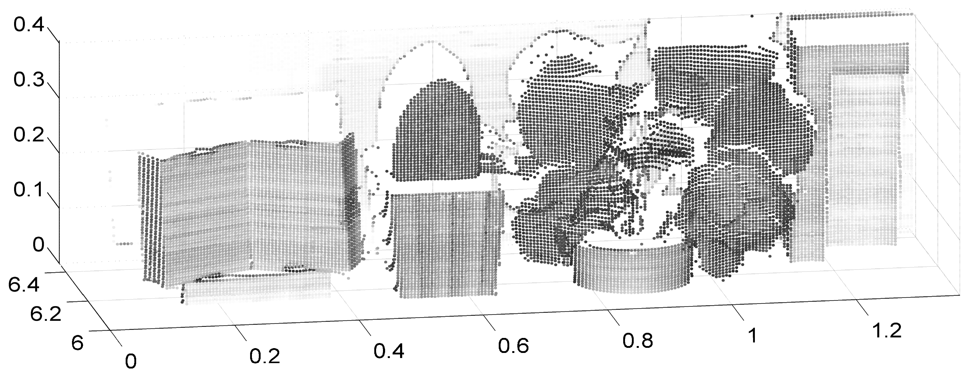
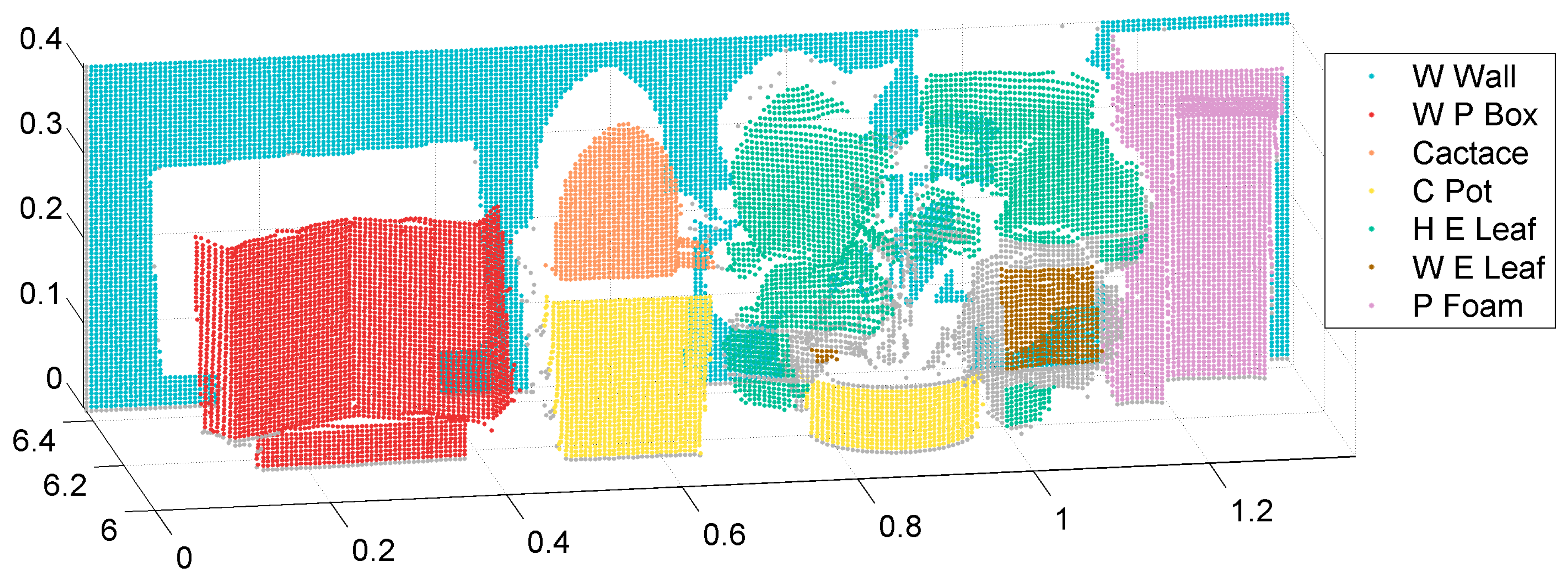
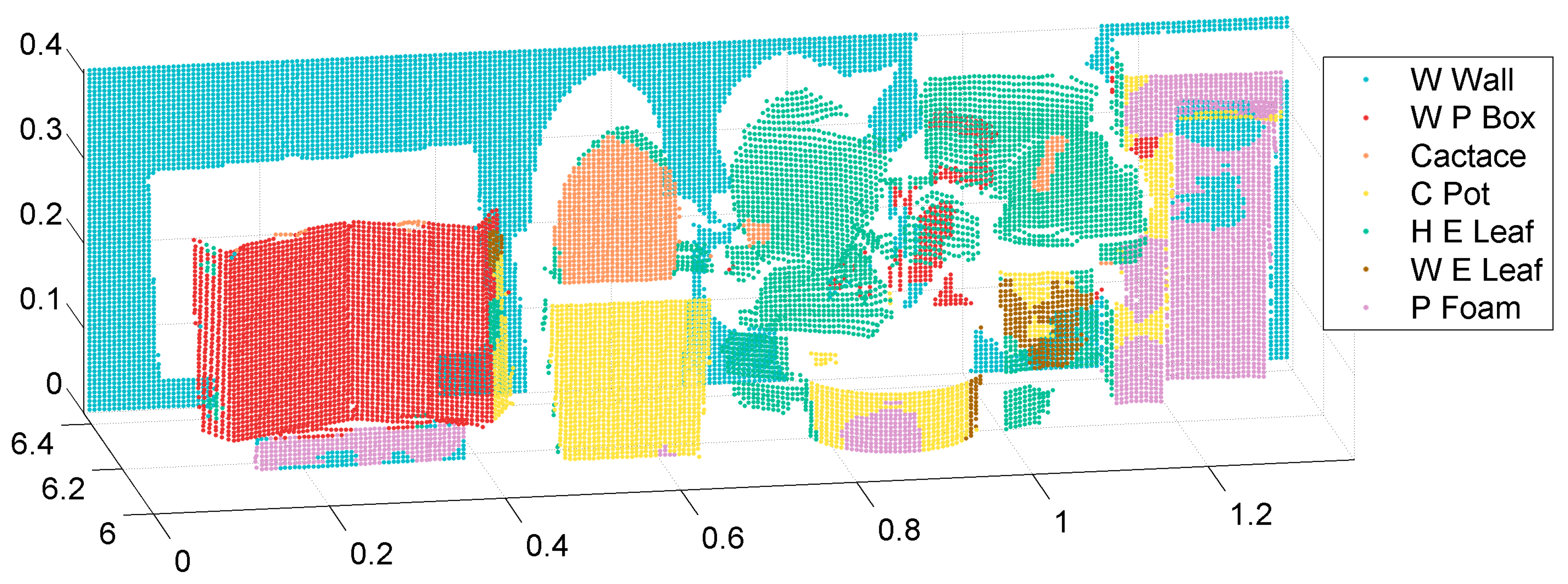
To evaluate classification accuracy, most points (92%) in the multispectral LiDAR point cloud were labeled manually using MATLAB software, with the spatial limitation for every target, as shown in Figure 4. Spatial outliers and points that were difficult to label manually were excluded (8%). The raw spectral reflectance of the multispectral LiDAR point cloud was normalized by spectraLon. SpectraLon is a fluoropolymer, and has the highest diffuse reflectance of any known material or coating over the ultraviolet, visible, and near-infrared regions of the spectrum [46]. An SVM classifier was used to train the classification model with the LibSVM proposed by Chang [47].
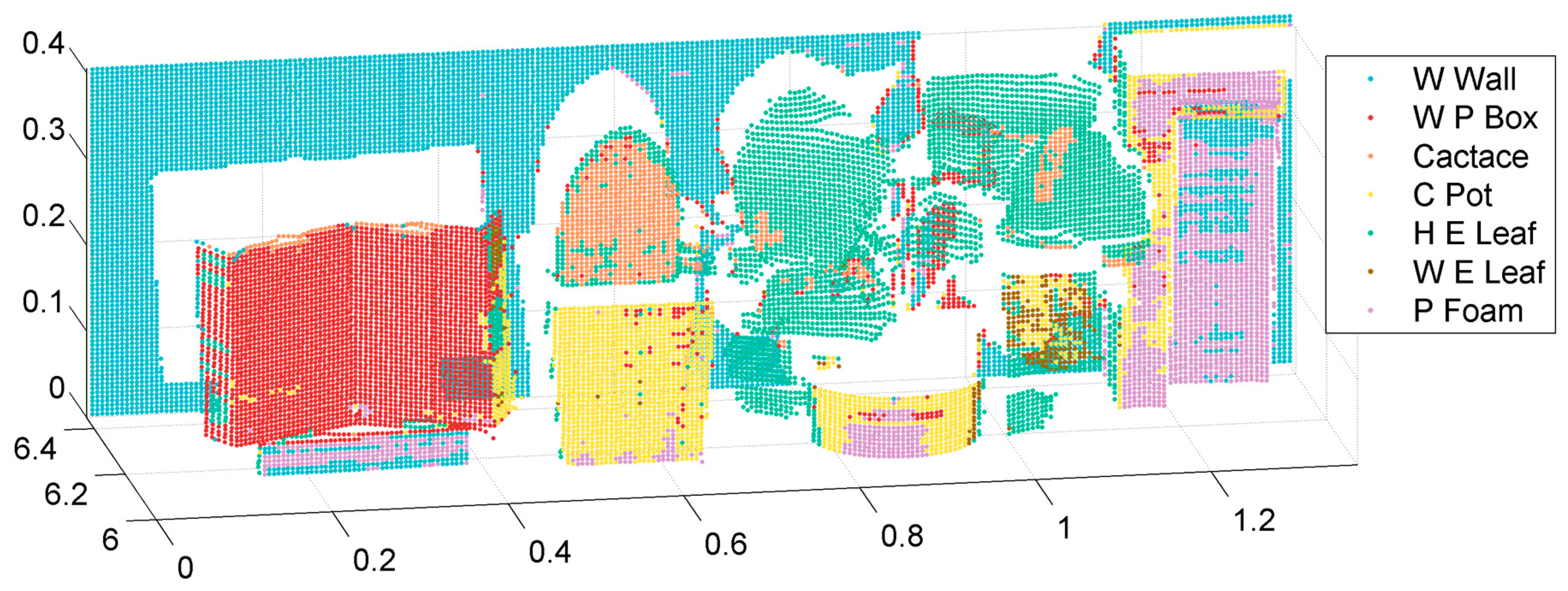
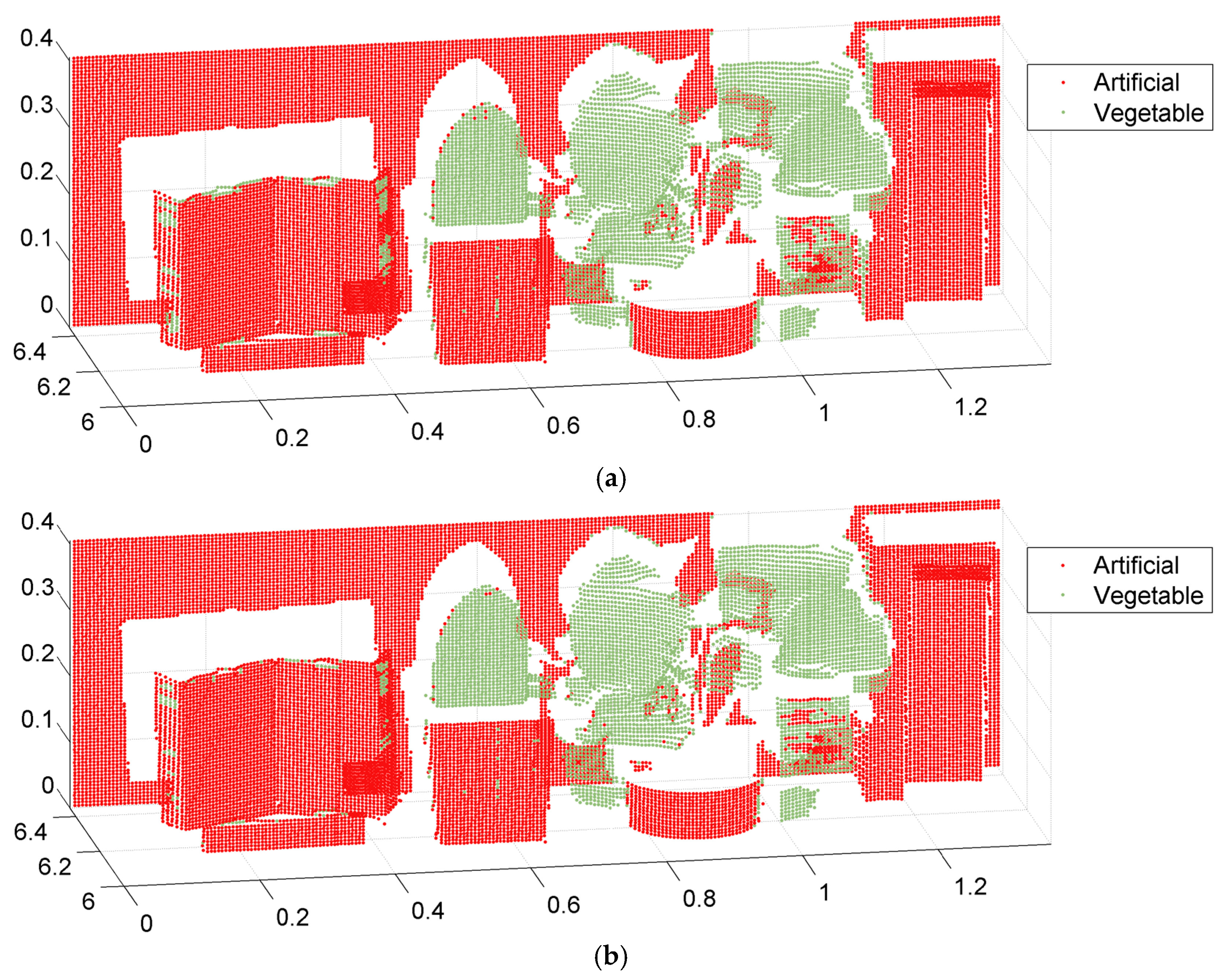
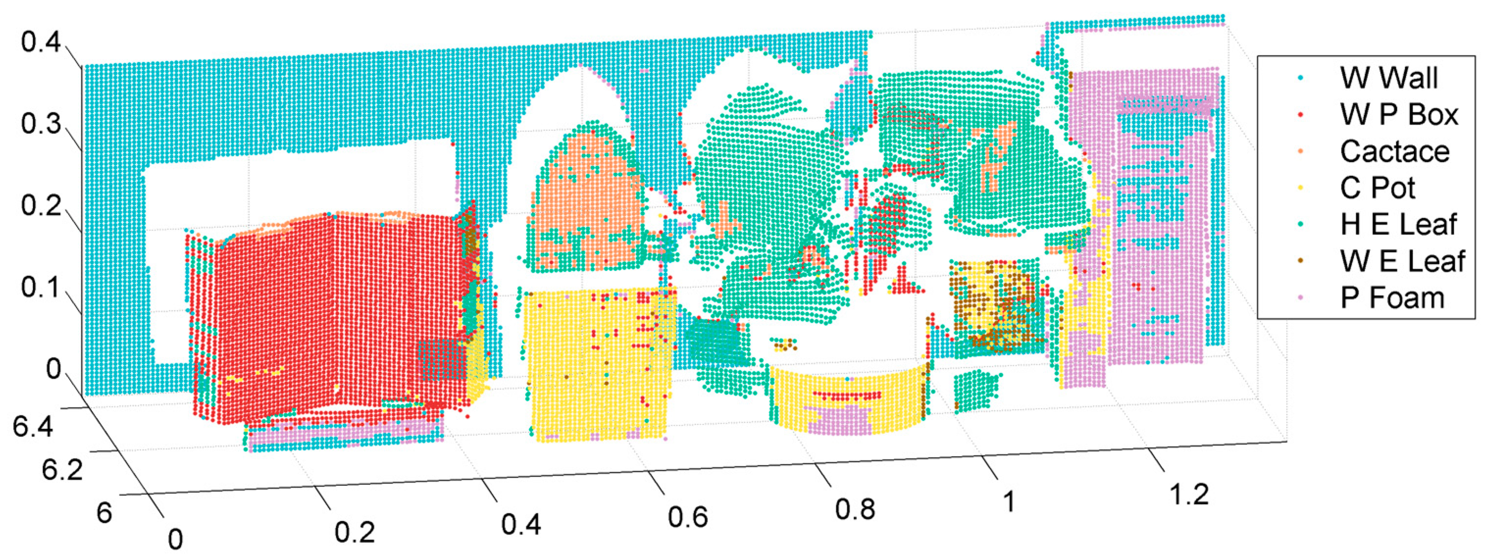
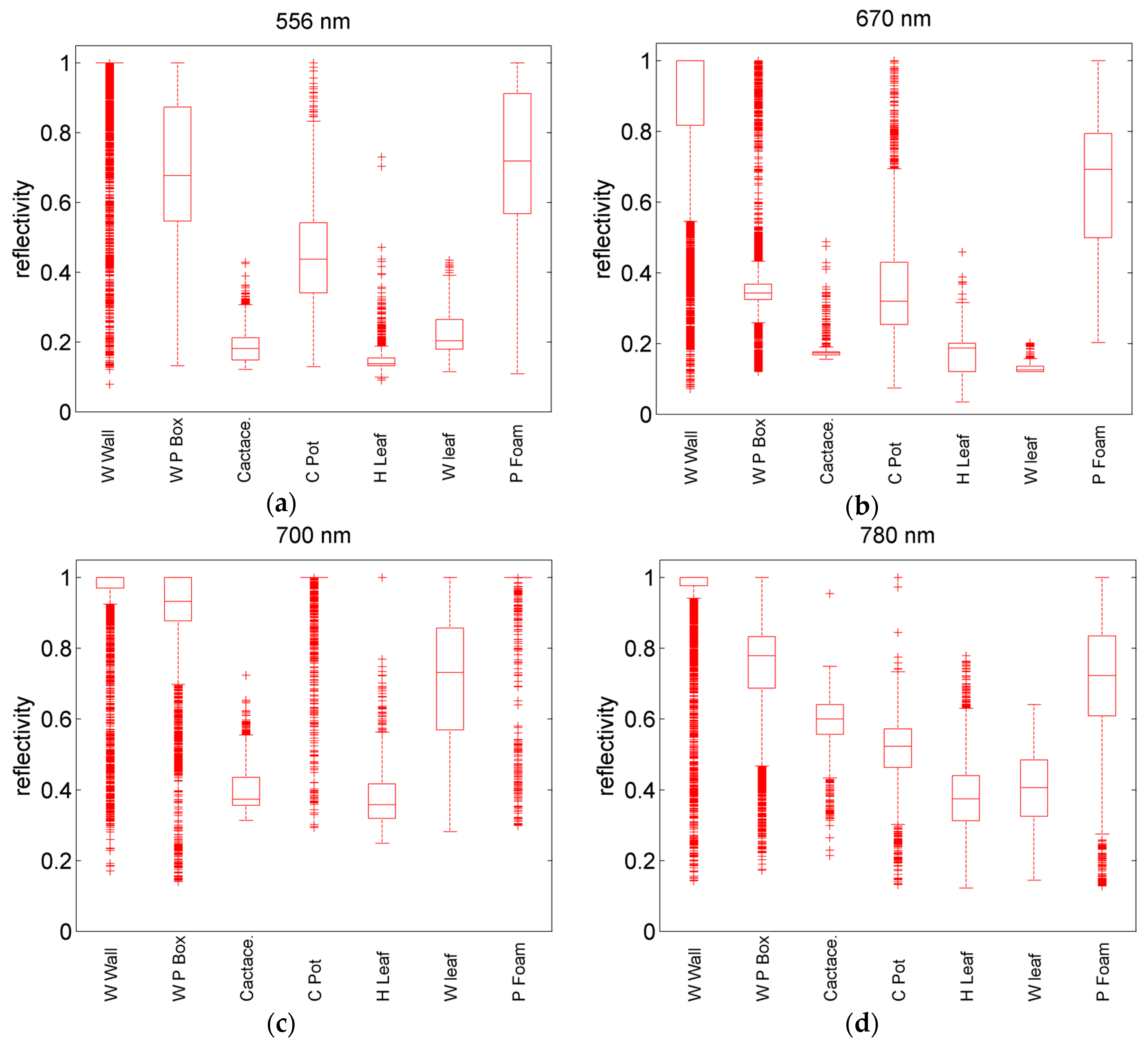
In this section, three classification sub-experiments were conducted with the use of raw spectral reflectance: (1) seven individual targets; (2) artificial (white wall, white paper box, ceramic flowerpot, plastic foam) and vegetable (cactus, healthy scindapsus leaves, withered scindapsus leaves) targets; and (3) healthy and withered scindapsus leaves. Training samples were a quarter of the total manually labeled points and were selected randomly with MATLAB. In this way, the spectral and spatial information of training samples were randomly distributed, and the integrity of training was ensured. The input parameters of the SVM classifier were four channels of raw spectral reflectance (556, 670, 700, and 780 nm). Results are shown in Figures 5, 6, and 8 in Section 4.

3.2. Classification Based on Vegetation Index (VI)

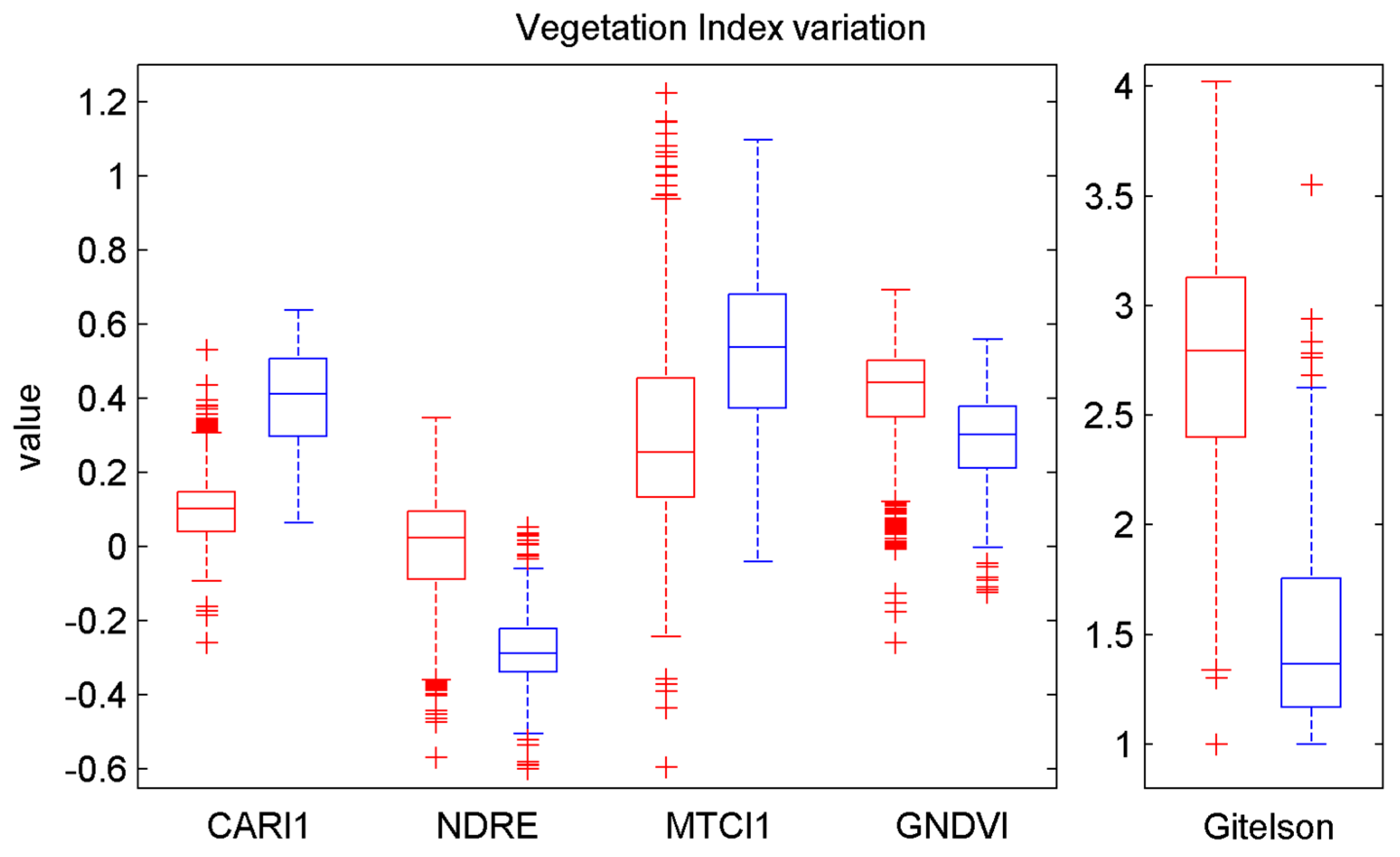
To enhance the capability of distinguishing artificial, healthy, and withered vegetable targets, VI was introduced to the classification. A VI is a spectral transformation of two or more bands designed to enhance the contribution of vegetation properties and allow reliable spatial and temporal inter-comparisons of terrestrial photosynthetic activity and canopy structural variations [48]. In consideration of the four wavelengths of the MWCL, namely, 556, 670, 700, and 780 nm, 14 types of VI were tested for the experiment separately, and are listed in Table 1 and Appendix A. A comparison among the classification results obtained by every single VI indicated that five VIs performed best; and were therefore selected as the input parameters of the SVM. The defined wavelengths in the original formula were replaced by the closest adapted wavelengths of the MWCL. The five VIs were calculated by the MWCL adapted formula for every point. These were additional classification features related to the biochemistry status of the vegetation.
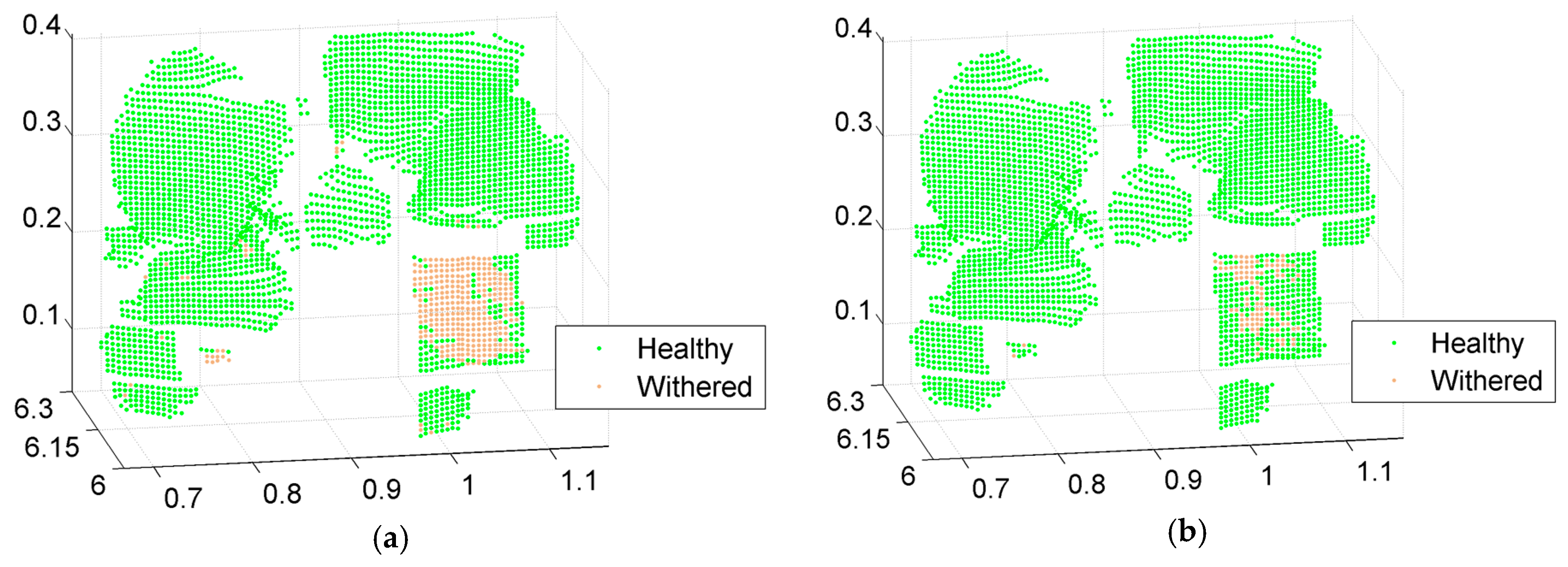
For this section, two classification sub-experiments were conducted with the use of the five VIs: (1) the artificial and vegetable targets; and (2) the healthy and withered scindapsus leaves. The training samples were the same as those in Section 3.1, and the classifier was SVM. Thus, only the input parameters were changed from Section 3.1 (from four channels of raw spectral reflectance to five channels of VI), thereby ensuring a comparison between the classification capability of VI and raw spectral reflectance.

3.3. Reclassification Based on Neighborhood Spatial Information with k-Nearest Neighbors Algorithm

After spectral information (raw spectral reflectance and VI) classification had allocated every point a class attribute, the k-NN classification algorithm was employed with the neighborhood spatial information for reclassification. The k-nearest neighbors algorithm is a non-parametric method for classification or regression [54]. In this experiment, the k-NN algorithm was used for classification in consideration of the nearest neighborhood point class.
Reclassification was based on the hypothesis that most of the neighborhood point class was correct after the first classification, where every point was assigned to the most common class considering its k (k is a positive integer) closest neighbors class attribute, in a fixed neighborhood distance. With a view to the scale of the targets, the density of point cloud, and the practical test, the k and neighborhood distance in this experiment were empirically set to 15 and two centimeters, respectively.
The two drawbacks of the k-NN algorithm are its sensitivity to the local samples of the data and the non-uniform distribution of samples. These two shortcomings can be overcome by the property of spatial distribution of the LiDAR point cloud. The distribution of one target in space is uninterrupted, thus, the points that describe one target are assembled in space. One point is usually surrounded by the points of the same target, and, furthermore, because of the steady scanning frequency, the density of points that describe one target is uniform.
Another advantage of employing k-NN to reclassify the multispectral LiDAR point cloud is the edge process. In images, most edges are surrounded by two or more classes of targets, thereby complicating the classification of the pixel on the edges. By contrast, most edges in a point cloud have only one class of target surrounding itself unless it is at the junction of different targets. Thus, the neighborhood points of the edge points are usually of the same class. Thus, the k-NN algorithm is suitable for the reclassification of the edges of the point cloud. The performance of k-NN is detailed in Section 4.3.

4. Results

4.1. Classification Based on Raw Spectral Reflectance

Figure 5 shows the classification result based on the raw spectral reflectance for seven individual targets. The salt and pepper noise is apparent in Figure 5. The overall accuracy was 81.258%; the confusion matrix is shown in Table 2. The confusion matrix shows that the user accuracies of most classes were more than 70%, but some of the producer accuracies were less than 70%: 40.4157% for withered scindapsus leaves and 62.8243% for plastic foam. With regard to the withered scindapsus leaves, 25.64% and 32.10% of points were classified as ceramic flowerpot and healthy scindapsus leaves, respectively, possibly because they were similar in the spectral feature space. Given the significant fluctuation of the reflectance of plastic foam over three wavelengths (Figure 3), precisely describing the spectral feature of plastic foam was difficult. Therefore, the classification result for plastic foam was not acceptable.
In addition, there were many error points at the edges of targets. For example, some points along the edges of the cactus were classified as healthy scindapsus leaves, and some points on the edges of the white wall were also falsely classified. Two main reasons explain these errors: first, the normal vector of the surface changes at the edge of the targets. Thus the scattering solid angle correspondingly changes, and a factor in raw spectral reflectance [55]. Second, the foot point of the beam may illuminate two or more targets simultaneously at the edges, and the echo reflectance combines echoes from different targets. Therefore, these types of points are difficult to classify and should be classified using spectral mixture analysis.
In the classification of artificial and vegetable targets, the cactus and scindapsus leaves were treated as vegetable targets and the others as artificial targets. The result based on raw spectral reflectance was satisfactory: overall accuracy was 96.457%. The classification result is shown in Figure 6a beside the result produced by VI (Figure 6b). Excluding individual noisy error points, there were main areas of error: the paper box; the withered scindapsus leaves; and the left edge of the plastic foam. The errors in the paper box and plastic foam are likely due to the changing incidence angle. Therefore, the correlation between the incidence angle and spectral reflectance requires further research. The errors seen in the withered leaves might result from the biochemical status of withered leaves when leaves change, thereby resulting in different spectral properties.
The classification result of healthy and withered scindapsus leaves on the basis of raw spectral reflectance and result obtained by VI are shown (Figure 8) in Section 4.2, for comparative purposes.

4.2. Classification Based on VI

In the classification of artificial and vegetable targets by VI, the accuracy was slightly better than that of raw spectral reflectance: 97.747% to 96.457%. The classification results are shown in Figure 6b. These experiments demonstrated that the MWCL could effectively classify artificial and vegetable objects using both raw spectral reflectance and VI.
For the classification of healthy and withered scindapsus leaves, the variance of five VIs of every point in healthy and withered scindapsus leaves is shown in Figure 7. Healthy and withered scindapsus leaves performed differently during every VI experiment. The variation in the distribution of the VI values for healthy and withered leaves was most significant in the case of CARI1, NDRE, and Gitelson, and merely noticeable in the case of MTCI1 and GNDVI.
The behaviors of healthy and withered scindapsus leaves on the spectrum are sharply different, especially in the visible region as seen in the photo (Figure 1). However, on scindapsus the classification result based on raw spectral reflectance was less accurate than that of the VI (Table 3). The result (Figure 8) indicates that the classification accuracy of VI (95.556%) was much better than that of raw spectral reflectance (90.039%), possibly because the VI could describe the biochemical status of leaves more precisely. In addition, NDRE and GNDVI could help remove the effect of incidence angle [55]. In particular, the VI was more helpful than raw spectral reflectance for recognizing withered scindapsus leaves (70.507%) while the accuracy of raw spectral reflectance was as low as 23.272%, as shown in Figure 8. This experiment demonstrated that the VI could be used by MWCL to classify healthy and withered scindapsus leaves, and increase the accuracy when recognizing withered scindapsus leaves in terms of raw spectral reflectance.

4.3. Reclassification Based on Neighborhood Spatial Information with k-NN

Reclassification was conducted after every spectral classification experiment, based on raw spectral reflectance and VI. The reclassification results obtained by k-NN with neighborhood spatial information are shown in Table 4. The k-NN algorithm helped to increase the classification accuracy in most experiments by 1.50–11.06% except in the recognition of withered scindapsus leaves by raw spectral reflectance due to the low first classification accuracy (23.272%). The results demonstrate that the k-NN algorithm with neighborhood spatial information performed well in most situations if the first spectra-based classification accuracy is reasonable.
If the first spectra-based classification accuracy of one class is too low, the neighborhood class attributes of most points of this class will be wrong. In k-NN, every point is assigned to the most common class of neighborhood points, considering its k (k is a positive integer) nearest neighbor class attribute. Therefore, the k-NN algorithm with neighborhood spatial information cannot work in this low first classification accuracy situation. That explains the declination of the classification accuracy of withered leaves based on raw spectral reflectance.
We analyzed the performance of the k-NN on a complex scene containing seven individual targets. After employing the k-NN algorithm with the neighborhood spatial information, the overall accuracy increased from 81.258% to 87.188%. Figure 9 shows the reclassification result, and the confusion matrix is presented in Table 5. A comparison with Table 2 shows increased producer and user accuracies, and a higher number of correctly classified points for every target.
The effect of the k-NN algorithm with neighborhood spatial information for the multispectral LiDAR point cloud is similar to that of image smoothing. This method corrects most falsely classified edge points, especially for the edges of the white wall. Scattered falsely classified points far away from edges were also corrected. The salt and pepper noise was mitigated. However, the large error area could not be corrected, and even some correct points that surrounded it were reclassified erroneously. This false reclassification may be a disadvantage of the k-NN algorithm with neighborhood spatial information, despite the evident increase in accuracy.
After the reclassification of seven individual targets, 11.83% of the points changed class: 8.88% were reclassified correctly, and 2.95% were reclassified falsely. These points are shown in Figure 10; where the green and red points denote the correctly and falsely reclassified points. The changed points were discretely distributed throughout the area, but no large error area with significant changes was found, thereby indicating that a large error area would not be corrected by the k-NN algorithm.

5. Discussion

The proposed two-step method was compared with the Gong method [38]. In Gong’s method, multispectral LiDAR point cloud was classified with the SVM. There were five dimensions of input parameters of the SVM: four for spectra, one for distance. Thus, the spatial information was not adequately used, and only used as one dimension of the input parameter of the SVM. For fair comparison, the training points were the same as those in our proposed two-step method. Therefore, the classification result of Gong’s method in this paper was slightly different from the result in Reference [38]. The confusion matrix and results are shown in Table 6 and Figure 11.
When comparing Table 5 and Table 6, our proposed two-step method had higher both user and producer accuracy for every class than via Gong’s method, except for the user accuracy of plastic foam. The lower user accuracy of plastic foam may be due to its great reflectance fluctuations at 556, 670 and 780 nm. However, in terms of the number of correctly classified points for plastic foam, our proposed method was better (1659 to 1639) and also the overall accuracy (87.188%) was higher than Gong’s method (82.797%).
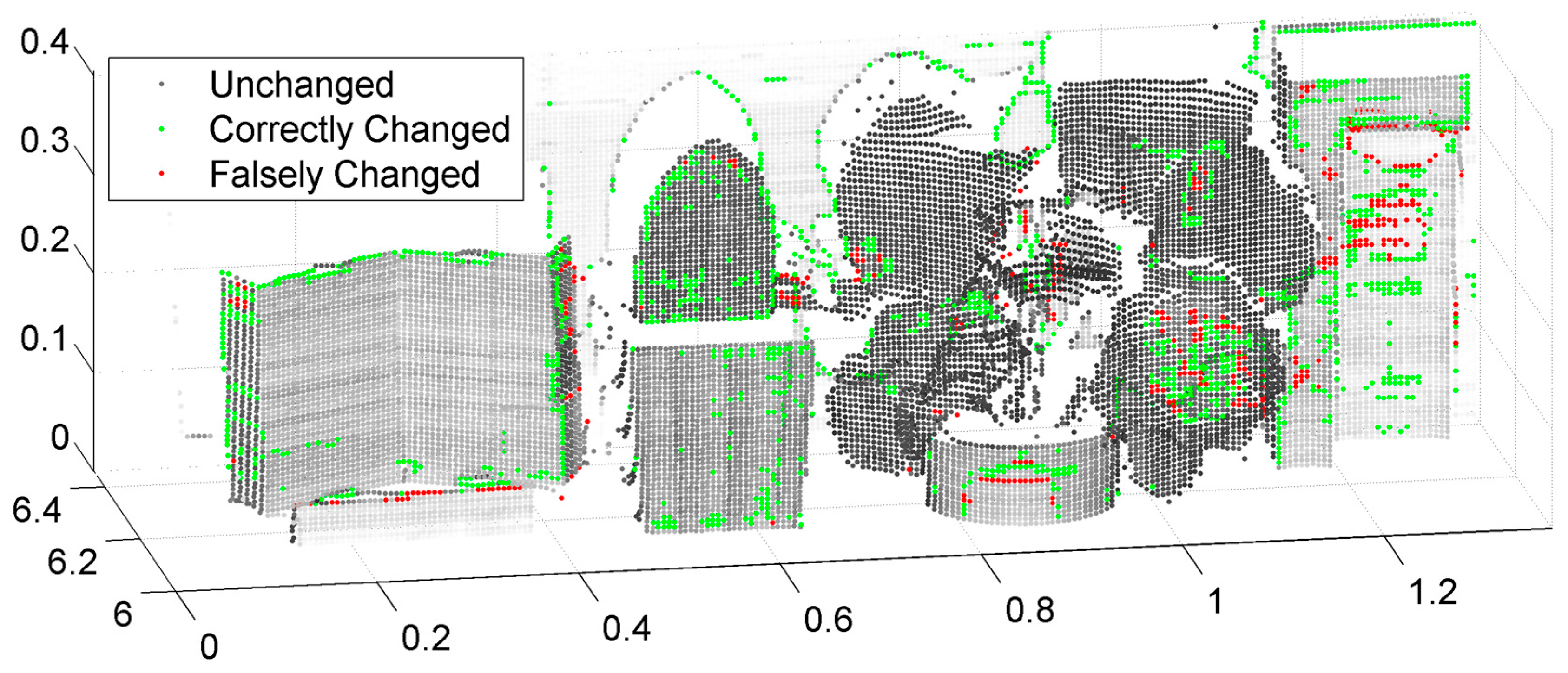
When comparing Figure 9 and Figure 11, the distribution of erroneously classified points was similar to our proposed method. The reason may be due to the role played by the spectral information in these two methods. Furthermore, the spectral information quality was actually not ideal in the area of error. In addition, there are many scatter error points in Gong’s method (Figure 11), unlike the result seen in Figure 9 classified by our two-step method. This also demonstrates the effectiveness of the k-NN algorithm with neighborhood spatial information.
The demerit of this two-step approach is that it cannot increase the classification accuracy if the first spectral classification accuracy is low. If the first classification accuracy of one class was low, then the class attributes of most neighborhood points will be wrong. The principle of k-NN is that every point was assigned to the most common class of neighborhood points, considering its k (k is a positive integer) closest neighbors class attribute. Therefore, the k-NN algorithm by neighborhood spatial information cannot work in this low spectral classification accuracy situation.

6. Conclusions

The data form of the multispectral LiDAR point cloud is unique because of its combination of spatial and spectral information, which is helpful for target classification. The properties of the data ensure that targets can be classified; first by using spectral information and then reclassified by using neighborhood spatial information. Experiments demonstrate the feasibility of this two-step classification method for multispectral LiDAR point cloud in most scenarios.
The first classification based on raw spectral reflectance performed well in most scenarios, aside from the classification of healthy and withered scindapsus leaves. After using the vegetation index, the classification accuracy of artificial and vegetable targets did not increase considerably. However, the overall classification accuracy of healthy and withered scindapsus leaves increased from 90.039% to 95.556%, compared with that obtained by raw spectral reflectance. For the identification of the withered scindapsus leaves, the accuracy increased from 23.272% to 70.507%, thereby indicating that vegetation indexes are more effective in classifying healthy and withered scindapsus leaves by multispectral LiDAR.
An analysis of the reclassification experiments indicates that the k-nearest neighbors algorithm with neighborhood spatial information can mitigate the salt and pepper noise and increase accuracy in most scenarios unless the first spectral classification accuracy was too low. Producer and user accuracies of every target rose in the confusion matrix in the seven-target classification (Table 1 and Table 2). The k-nearest neighbor algorithm in conjunction with neighborhood spatial information performed well in raw spectral reflectance and in the vegetation index experiments in most cases (overall accuracies increased by 1.50–11.06%). These results show that the proposed two-step classification method is feasible for multispectral LiDAR point clouds and that the k-nearest neighbor algorithm with neighborhood spatial information is an effective tool for increasing classification accuracy.
One disadvantage of this method is that the k-nearest neighbors algorithm with neighborhood spatial information will not work in low first spectral-information-based classification accuracy situations. In addition, it was conducted in a laboratory and the experimental targets were limited. Further outdoor experiments with more complicated targets would be required to complete the assessment of its feasibility.
Furthermore, a better algorithm for the spatial information to increase classification accuracy requires more research to utilize the spatial information more adequately. For example, the spectral-spatial method for hyperspectral imagery might be considered for the introduction for multispectral LiDAR. In addition, research on object and point classification, and the internal relation of object and point classification for multispectral LiDAR will be conducted.

Acknowledgments

This study was supported by the National Natural Science Foundation of China (Grant No. 41601360; 41611130114; 41571370); the Natural Science Foundation of Hubei Province (Grant No. 2015CFA002); the Fundamental Research Funds for the Central Universities (Grant No. 2042016kf0008); and the Open Research Fund of State Key Laboratory of Information Engineering in Surveying, Mapping and Remote Sensing (Grant No. 15R01).

Author Contributions

Wei Gong and Biwu Chen conceived and designed the experiments; Shuo Shi, Qingjun Zhang, Shalei Song, and Zhenbing Zhang performed the experiments; Biwu Chen analyzed the data; Jia Sun, Jian Yang and Lin Du contributed analysis tools; Biwu Chen wrote the paper.

Conflicts of Interest

The authors declare no conflict of interest.

Appendix A

Table A1. Other nine vegetation indexes except the selected five ones.
Vegetation IndexMWCL Adapted FormulaOriginal Formula
Triangle Vegetation Index (TVI) [56]0.5 × [120 × (R780 − R556) − 200 × (R670 − R556)]0.5 × [120 × (NIR − GREEN) –200 × (R − GREEN)]
Red-edge Triangular Vegetation Index (RTVI) [57][100 × (R780 − R700) – 10 × (R780 − R556)] sqrt (R700/R670)[100 × (R750 − R730) – 10 × (R750 − R550)] sqrt (R700/R670)
Modified Chlorophyll Absorption in Reflectance Index (MCARI) [58][(R700 − R670) − 0.2 × (R700 − R556)](R700/R670)[(R700 − R670) − 0.2 × (R700 − R550)](R700/R670)
Transformed Chlorophyll Absorption in Reflectance Index (TCARI) [59]3 × [(R700 − R670) − 0.2 × (R700 − R556)(R700/R670)]3 × [(R700 − R670) − 0.2 × (R700 − R550)(R700/R670)]
Red-edge Inflection Point (REIP) [60]700 + 40 × [(R670 + R780)/2 − R700]/(R780 − R700)700 + 40 × [(R670 + R780)/2 − R700]/(R740 − R700)
Normalized Difference Vegetation Index (NDVI) [61](R780 − R670)/(R780 + R670)(NIR − R)/(NIR + R)
Soil-Adjusted Vegetation Index (SAVI) [62][(R780 – R670)/(R780 + R670 + 0.5)] × (1 + 0.5)[(NIR − R)/(NIR + R + 0.5)] × (1 + 0.5)
Optimized Soil-Adjusted Vegetation Index (OSAVI) [63][(R780 – R670)/(R780 + R670 + 0.16)][(NIR − R)/(NIR + R + 0.16)]
Optimal Vegetation Index (VIopt) [64](1 + 0.45)((R780)2 + 1)/(R670 + 0.45)(1 + 0.45)((NIR)2 + 1)/(R + 0.45)

References

  1. Brekke, C.; Solberg, A.H.S. Oil spill detection by satellite remote sensing. Remote Sens. Environ. 2005, 95, 1–13. [Google Scholar] [CrossRef]
  2. Ricchetti, E. Multispectral satellite image and ancillary data integration for geological classification. Photogramm. Eng. Remote Sens. 2000, 66, 429–435. [Google Scholar]
  3. Li, C.; Wang, J.; Wang, L.; Hu, L.; Gong, P. Comparison of classification algorithms and training sample sizes in urban land classification with landsat thematic mapper imagery. Remote Sens. 2014, 6, 964. [Google Scholar] [CrossRef]
  4. Wardlow, B.D.; Egbert, S.L.; Kastens, J.H. Analysis of time-series modis 250 m vegetation index data for crop classification in the U.S. Central great plains. Remote Sens. Environ. 2007, 108, 290–310. [Google Scholar] [CrossRef]
  5. Yang, J.; Shi, S.; Gong, W.; Du, L.; Ma, Y.Y.; Zhu, B.; Song, S.L. Application of fluorescence spectrum to precisely inverse paddy rice nitrogen content. Plant Soil Environ. 2015, 61, 182–188. [Google Scholar] [CrossRef]
  6. Koch, B.; Heyder, U.; Weinacker, H. Detection of individual tree crowns in airborne LiDAR data. Photogramm. Eng. Remote Sens. 2006, 72, 357–363. [Google Scholar] [CrossRef]
  7. Immitzer, M.; Atzberger, C.; Koukal, T. Tree species classification with random forest using very high spatial resolution 8-band worldview-2 satellite data. Remote Sens. 2012, 4, 2661. [Google Scholar] [CrossRef]
  8. Wolter, P.T.; Mladenoff, D.J.; Host, G.E.; Crow, T.R. Improved forest classification in the northern lake states using multi-temporal landsat imagery. Photogramm. Eng. Remote Sens. 1995, 61, 1129–1144. [Google Scholar]
  9. Ramsey, E.; Rangoonwala, A.; Jones, C. Structural classification of marshes with polarimetric sar highlighting the temporal mapping of marshes exposed to oil. Remote Sens. 2015, 7, 11295. [Google Scholar] [CrossRef]
  10. Zhou, G.; Zhang, R.; Zhang, D. Manifold learning co-location decision tree for remotely sensed imagery classification. Remote Sens. 2016, 8, 855. [Google Scholar] [CrossRef]
  11. Yang, J.; Gong, W.; Shi, S.; Du, L.; Sun, J.; Song, S.L. Estimation of nitrogen content based on fluorescence spectrum and principal component analysis in paddy rice. Plant Soil Environ. 2016, 62, 178–183. [Google Scholar] [CrossRef]
  12. Serpico, S.B.; Bruzzone, L.; Roli, F. Special issue on non-conventional pattern analysis in remote sensingan experimental comparison of neural and statistical non-parametric algorithms for supervised classification of remote-sensing images. Pattern Recognit. Lett. 1996, 17, 1331–1341. [Google Scholar] [CrossRef]
  13. Licciardi, G.; Pacifici, F.; Tuia, D.; Prasad, S.; West, T.; Giacco, F.; Thiel, C.; Inglada, J.; Christophe, E.; Chanussot, J.; Gamba, P. Decision fusion for the classification of hyperspectral data: Outcome of the 2008 GRS-S data fusion contest. IEEE Trans. Geosci. Remote Sens. 2009, 47, 3857–3865. [Google Scholar] [CrossRef]
  14. Yang, J.; Gong, W.; Shi, S.; Du, L.; Sun, J.; Ma, Y.; Song, S. Accurate identification of nitrogen fertilizer application of paddy rice using laser-induced fluorescence combined with support vector machine. Plant Soil Environ. 2015, 61, 501–506. [Google Scholar] [CrossRef]
  15. Wieland, M.; Liu, W.; Yamazaki, F. Learning change from synthetic aperture radar images: Performance evaluation of a support vector machine to detect earthquake and tsunami-induced changes. Remote Sens. 2016, 8, 792. [Google Scholar] [CrossRef]
  16. Chen, J.; Wang, C.; Wang, R. Using stacked generalization to combine svms in magnitude and shape feature spaces for classification of hyperspectral data. IEEE Trans. Geosci. Remote Sens. 2009, 47, 2193–2205. [Google Scholar] [CrossRef]
  17. Marconcini, M.; Camps-Valls, G.; Bruzzone, L. A composite semisupervised svm for classification of hyperspectral images. IEEE Geosci. Remote Sens. Lett. 2009, 6, 234–238. [Google Scholar] [CrossRef]
  18. Chen, J.; Wang, C.; Wang, R. Fusion of svms in wavelet domain for hyperspectral data classification. In Proceedings of the 2009 IEEE International Conference on Robotics and Biomimetics (ROBIO), Guilin, China, 19–23 December 2009; pp. 1372–1375. [Google Scholar]
  19. Demir, B.; Erturk, S. Clustering-based extraction of border training patterns for accurate svm classification of hyperspectral images. IEEE Geosci. Remote Sens. Lett. 2009, 6, 840–844. [Google Scholar] [CrossRef]
  20. Mountrakis, G.; Im, J.; Ogole, C. Support vector machines in remote sensing: A review. ISPRS J. Photogramm. Remote Sens. 2011, 66, 247–259. [Google Scholar] [CrossRef]
  21. Zhan, Q.; Molenaar, M.; Tempfli, K. Building extraction from laser data by reasoning on image segments in elevation slices. Int. Arch. Photogramm. Remote Sens. Spat. Inf. Sci. 2002, 34, 305–308. [Google Scholar]
  22. Brodu, N.; Lague, D. 3D terrestrial LiDAR data classification of complex natural scenes using a multi-scale dimensionality criterion: Applications in geomorphology. ISPRS J. Photogramm. Remote Sens. 2012, 68, 121–134. [Google Scholar] [CrossRef]
  23. Vaughn, N.R.; Moskal, L.M.; Turnblom, E.C. Tree species detection accuracies using discrete point LiDAR and airborne waveform LiDAR. Remote Sens. 2012, 4, 377. [Google Scholar] [CrossRef]
  24. Guo, L.; Chehata, N.; Mallet, C.; Boukir, S. Relevance of airborne LiDAR and multispectral image data for urban scene classification using random forests. ISPRS J. Photogramm. Remote Sens. 2011, 66, 56–66. [Google Scholar] [CrossRef]
  25. García, M.; Riaño, D.; Chuvieco, E.; Salas, J.; Danson, F.M. Multispectral and LiDAR data fusion for fuel type mapping using support vector machine and decision rules. Remote Sens. Environ. 2011, 115, 1369–1379. [Google Scholar] [CrossRef]
  26. Laible, S.; Khan, Y.N.; Bohlmann, K.; Zell, A. 3D LiDAR- and camera-based terrain classification under different lighting conditions. In Autonomous Mobile Systems; Springer: Berlin/Heidelberg, Germany, 2012; pp. 21–29. [Google Scholar]
  27. Zhang, J.; Lin, X. Advances in fusion of optical imagery and LiDAR point cloud applied to photogrammetry and remote sensing. Int. J. Image Data Fusion 2016, 8, 1–31. [Google Scholar] [CrossRef]
  28. Wei, G.; Shalei, S.; Bo, Z.; Shuo, S.; Faquan, L.; Xuewu, C. Multi-wavelength canopy LiDAR for remote sensing of vegetation: Design and system performance. ISPRS J. Photogramm. Remote Sens. 2012, 69, 1–9. [Google Scholar] [CrossRef]
  29. Niu, Z.; Xu, Z.; Sun, G.; Huang, W.; Wang, L.; Feng, M.; Li, W.; He, W.; Gao, S. Design of a new multispectral waveform LiDAR instrument to monitor vegetation. IEEE Geosci. Remote Sens. Lett. 2015, 12, 1506–1510. [Google Scholar]
  30. Woodhouse, I.H.; Nichol, C.; Sinclair, P.; Jack, J.; Morsdorf, F.; Malthus, T.J.; Patenaude, G. A multispectral canopy LiDAR demonstrator project. IEEE Geosci. Remote Sens. Lett. 2011, 8, 839–843. [Google Scholar] [CrossRef]
  31. Li, W.; Sun, G.; Niu, Z.; Gao, S.; Qiao, H. Estimation of leaf biochemical content using a novel hyperspectral full-waveform LiDAR system. Remote Sens. Lett. 2014, 5, 693–702. [Google Scholar] [CrossRef]
  32. Nevalainen, O.; Hakala, T.; Suomalainen, J.; Mäkipää, R.; Peltoniemi, M.; Krooks, A.; Kaasalainen, S. Fast and nondestructive method for leaf level chlorophyll estimation using hyperspectral LiDAR. Agric. For. Meteorol. 2014, 198, 250–258. [Google Scholar] [CrossRef]
  33. Du, L.; Gong, W.; Shi, S.; Yang, J.; Sun, J.; Zhu, B.; Song, S. Estimation of rice leaf nitrogen contents based on hyperspectral LiDAR. Int. J. Appl. Earth Obs. Geoinf. 2016, 44, 136–143. [Google Scholar] [CrossRef]
  34. Wichmann, V.; Bremer, M.; Lindenberger, J.; Rutzinger, M.; Georges, C.; Petrini-Monteferri, F. Evaluating the potential of multispectral airborne LiDAR for topographic mapping and land cover classification. ISPRS Ann. Photogramm. Remote Sens. Spat. Inf. Sci. 2015, II-3/W5, 113–119. [Google Scholar] [CrossRef]
  35. Zou, X.; Zhao, G.; Li, J.; Yang, Y.; Fang, Y. 3D land cover classification based on multispectral LiDAR point clouds. ISPRS Int. Arch. Photogramm. Remote Sens. Spat. Inf. Sci. 2016, XLI-B1, 741–747. [Google Scholar]
  36. Ahokas, E.; Hyyppä, J.; Yu, X.; Liang, X.; Matikainen, L.; Karila, K.; Litkey, P.; Kukko, A.; Jaakkola, A.; Kaartinen, H. Towards automatic single-sensor mapping by multispectral airborne laser scanning. ISPRS Int. Arch. Photogramm. Remote Sens. Spat. Inf. Sci. 2016, XLI-B3, 155–162. [Google Scholar]
  37. Hartzell, P.; Glennie, C.; Biber, K.; Khan, S. Application of multispectral LiDAR to automated virtual outcrop geology. ISPRS J. Photogramm. Remote Sens. 2014, 88, 147–155. [Google Scholar] [CrossRef]
  38. Gong, W.; Sun, J.; Shi, S.; Yang, J.; Du, L.; Zhu, B.; Song, S. Investigating the potential of using the spatial and spectral information of multispectral LiDAR for object classification. Sensors 2015, 15, 21989–22002. [Google Scholar] [CrossRef] [PubMed]
  39. Vauhkonen, J.; Hakala, T.; Suomalainen, J.; Kaasalainen, S.; Nevalainen, O.; Vastaranta, M.; Holopainen, M.; Hyyppa, J. Classification of spruce and pine trees using active hyperspectral LiDAR. IEEE Geosci. Remote Sens. Lett. 2013, 10, 1138–1141. [Google Scholar] [CrossRef]
  40. Tang, T.; Dai, L. Accuracy test of point-based and object-based urban building feature classification and extraction applying airborne LiDAR data. Geocarto Int. 2014, 29, 710–730. [Google Scholar] [CrossRef]
  41. Antonarakis, A.S.; Richards, K.S.; Brasington, J. Object-based land cover classification using airborne LiDAR. Remote Sens. Environ. 2008, 112, 2988–2998. [Google Scholar] [CrossRef]
  42. Wallace, A.; Nichol, C.; Woodhouse, I. Recovery of forest canopy parameters by inversion of multispectral LiDAR data. Remote Sens. 2012, 4, 509–531. [Google Scholar] [CrossRef]
  43. Bo, Z.; Wei, G.; Shi, S.; Song, S. A multi-wavelength canopy LiDAR for vegetation monitoring: System implementation and laboratory-based tests. Procedia Environ. Sci. 2011, 10, 2775–2782. [Google Scholar] [CrossRef]
  44. Biavati, G.; Donfrancesco, G.D.; Cairo, F.; Feist, D.G. Correction scheme for close-range LiDAR returns. Appl. Opt. 2011, 50, 5872–5882. [Google Scholar] [CrossRef] [PubMed]
  45. Kao, D.L.; Kramer, M.G.; Love, A.L.; Dungan, J.L.; Pang, A.T. Visualizing distributions from multi-return LiDAR data to understand forest structure. Cartogr. J. 2005, 42, 35–47. [Google Scholar] [CrossRef]
  46. Georgiev, G.T.; Butler, J.J. Long-term calibration monitoring of spectralon diffusers brdf in the air-ultraviolet. Appl. Opt. 2007, 46, 7892–7899. [Google Scholar] [CrossRef] [PubMed]
  47. Chang, C.-C.; Lin, C.-J. Libsvm: A library for support vector machines. ACM Trans. Intell. Syst. Technol. 2011, 2, 27. [Google Scholar] [CrossRef]
  48. Huete, A.; Didan, K.; Miura, T.; Rodriguez, E.P.; Gao, X.; Ferreira, L.G. Overview of the radiometric and biophysical performance of the modis vegetation indices. Remote Sens. Environ. 2002, 83, 195–213. [Google Scholar] [CrossRef]
  49. Kim, M.S.; Daughtry, C.; Chappelle, E.; McMurtrey, J.; Walthall, C. The use of high spectral resolution bands for estimating absorbed photosynthetically active radiation (a par). In Proceedings of the 6th International Symposium on Physical Measurements and Signatures in Remote Sensing, Val d’lsère, France, 17–21 January 1994. [Google Scholar]
  50. Barnes, E.; Clarke, T.; Richards, S.; Colaizzi, P.; Haberland, J.; Kostrzewski, M.; Waller, P.; Choi, C.; Riley, E.; Thompson, T. Coincident detection of crop water stress, nitrogen status and canopy density using ground based multispectral data. In Proceedings of the 5th International Conference on Precision Agriculture, Bloomington, MN, USA, 16–19 July 2000; pp. 16–19. [Google Scholar]
  51. Haboudane, D.; Miller, J.R.; Pattey, E.; Zarco-Tejada, P.J.; Strachan, I.B. Hyperspectral vegetation indices and novel algorithms for predicting green lai of crop canopies: Modeling and validation in the context of precision agriculture. Remote Sens. Environ. 2004, 90, 337–352. [Google Scholar] [CrossRef]
  52. Gitelson, A.A.; Buschmann, C.; Lichtenthaler, H.K. The chlorophyll fluorescence ratio f735/f700 as an accurate measure of the chlorophyll content in plants. Remote Sens. Environ. 1999, 69, 296–302. [Google Scholar] [CrossRef]
  53. Gitelson, A.A.; Kaufman, Y.J.; Merzlyak, M.N. Use of a green channel in remote sensing of global vegetation from eos-modis. Remote Sens. Environ. 1996, 58, 289–298. [Google Scholar] [CrossRef]
  54. Altman, N.S. An introduction to kernel and nearest-neighbor nonparametric regression. Am. Stat. 1992, 46, 175–185. [Google Scholar] [CrossRef]
  55. Shi, S.; Song, S.; Gong, W.; Du, L.; Zhu, B.; Huang, X. Improving backscatter intensity calibration for multispectral LiDAR. IEEE Geosci. Remote Sens. Lett. 2015, 12, 1421–1425. [Google Scholar] [CrossRef]
  56. Broge, N.H.; Leblanc, E. Comparing prediction power and stability of broadband and hyperspectral vegetation indices for estimation of green leaf area index and canopy chlorophyll density. Remote Sens. Environ. 2001, 76, 156–172. [Google Scholar] [CrossRef]
  57. Nicolas, T.; Philippe, V.; Huang, W.-J. New index for crop canopy fresh biomass estimation. Spectrosc. Spectr. Anal. 2010, 30, 512–517. [Google Scholar]
  58. Daughtry, C.; Walthall, C.; Kim, M.; De Colstoun, E.B.; McMurtrey, J. Estimating corn leaf chlorophyll concentration from leaf and canopy reflectance. Remote Sens. Environ. 2000, 74, 229–239. [Google Scholar] [CrossRef]
  59. Haboudane, D.; Miller, J.R.; Tremblay, N.; Zarco-Tejada, P.J.; Dextraze, L. Integrated narrow-band vegetation indices for prediction of crop chlorophyll content for application to precision agriculture. Remote Sens. Environ. 2002, 81, 416–426. [Google Scholar] [CrossRef]
  60. Guyot, G.; Baret, F.; Major, D. High spectral resolution: Determination of spectral shifts between the red and the near infrared. Int. Arch. Photogramm. Remote Sens. 1988, 11, 740–760. [Google Scholar]
  61. Rouse, J.W., Jr.; Haas, R.; Schell, J.; Deering, D. Monitoring Vegetation Systems in the Great Plains With Erts. Available online: https://ntrs.nasa.gov/search.jsp?R=19740022614 (accessed on 20 September 2016).
  62. Huete, A.R. A soil-adjusted vegetation index (savi). Remote Sens. Environ. 1988, 25, 295–309. [Google Scholar] [CrossRef]
  63. Rondeaux, G.; Steven, M.; Baret, F. Optimization of soil-adjusted vegetation indices. Remote Sens. Environ. 1996, 55, 95–107. [Google Scholar] [CrossRef]
  64. Reyniers, M.; Walvoort, D.J.J.; Baardemaaker, J.D. A linear model to predict with a multi-spectral radiometer the amount of nitrogen in winter wheat. Int. J. Remote Sens. 2006, 27, 4159–4178. [Google Scholar] [CrossRef]
Figure 1. Photo of the realistic experimental scene.
Remotesensing 09 00373 g001
Figure 2. Point cloud of the experimental materials. The white wall points are almost white for high reflectance, which is why they are nearly invisible in this picture.
Remotesensing 09 00373 g002
Figure 3. Normalized spectral reflectance variation of seven targets on four wavelengths: (a) 556; (b) 670; (c) 700; and (d) 780 nm. The upper, bottom edge, and middle line of the box represent the 25th and 75th percentiles, and the median of the point cloud, respectively. The length of the dotted line is 1.5 times that of the box unless the end of dotted line contains all external points. Outliers are marked with crosses.
Remotesensing 09 00373 g003
Figure 4. Manually labeled multispectral light detection and ranging (LiDAR) point cloud in the seven materials: white wall, white paper box, cactus, ceramic flowerpot, healthy scindapsus leaves, withered scindapsus leaves and plastic foam, which are shown in blue, red, orange, yellow, green, brown and purple, respectively.
Remotesensing 09 00373 g004
Figure 5. Classification results based on raw spectral reflectance. Different colors represent the different results of targets. The representative color is the same as the training samples shown in Figure 4.
Remotesensing 09 00373 g005
Figure 6. Classification of artificial (white wall, white paper box, ceramic flowerpot, and plastic foam) and vegetable (cactus and scindapsus leaves) targets on the basis of (a) raw spectral reflectance; and (b) five VIs. Red and green points represent the artificial and vegetable samples, respectively.
Remotesensing 09 00373 g006
Figure 7. Variation of the five types of vegetation indexes of healthy (red) and withered (blue) scindapsus leaves: Chlorophyll Absorption Reflectance Index 1, Normalized Difference Red Edge, Modified Triangular Vegetation Index 1, Green Normalized Difference Vegetation Index, and Gitelson. The upper, bottom edge, and middle line of the box represent the 25th and 75th percentiles, and the median of the VI value, respectively. The length of the dotted line is 1.5 times that of the box unless end of the dotted line contains the external point. Outliers are marked with red crosses.
Remotesensing 09 00373 g007
Figure 8. Healthy and withered scindapsus leaves classification results based on (a) VI and (b) spectral reflectance. Green and brown points indicate healthy and withered leaves, respectively. The result indicates that the VI is more sensitive to the growing condition of leaves, which makes it helpful for discriminating between healthy and withered leaves.
Remotesensing 09 00373 g008
Figure 9. Reclassification result of seven individual targets based on the k-NN algorithm with spatial information. Different colors represent different targets. The representative colors are the same as those of the training samples in Figure 4.
Remotesensing 09 00373 g009
Figure 10. Colorful points represent the points whose class changed after reclassification based on the k-NN algorithm with spatial information. Gray, green, and red points represent the unchanged points, the correctly changed points, and the falsely changed points, respectively.
Remotesensing 09 00373 g010
Figure 11. Classification result of the seven individual targets based on Gong’s method [38]. Different colors represent different targets. The representative colors are the same as those of the training samples in Figure 4.
Remotesensing 09 00373 g011
Table 1. Details of five selected vegetation indices (VIs).
Vegetation IndexMWCL Adapted FormulaOriginal Formula
Chlorophyll Absorption Reflectance Index 1 (CARI1) [49](R700 − R670) − 0.2 × (R700 + R556)(R700 − R670) − 0.2 × (R700 + R550)
Normalized Difference Red Edge (NDRE) [50](R780 − R700)/(R780 + R700)(R790 − R720)/(R790 + R720)
Modified Triangular Vegetation Index1 (MTVI1) [51]1.2 × [1.2 × (R780 − R556) − 2.5 × (R670 − R556)]1.2 × [1.2 × (R800 − R550) − 2.5 × (R670 − R550)]
Gitelson [52]1/R7001/R700
Green Normalized Difference Vegetation Index (GNDVI) [53](R780 − R556)/(R780 + R556)(NIR − GREEN)/(NIR + GREEN)
Table 2. Confusion matrix of the classification based on raw spectral reflectance.
Predicted ClassProducer Accuracy
W WallW P BoxCactus.C PotH E LeafW E LeafP Foam
Ground truthW Wall548635097410641300.8907
W P Box187278473150134352000.7813
Cactus.1176250213000.7301
C Pot3690140168272110.7875
H E Leaf01417312728400.9342
W E Leaf06211113917500.4041
Plastic F36472134589314770.6282
User accuracy0.90810.84050.70780.67290.78450.70560.7319
Table 3. Confusion matrixes of the classification of healthy and withered scindapsus leaves, based on the VI (left) and raw spectral reflectance (right).
VIRaw Spectral Reflectance
Predicted ClassProducer AccuracyPredicted ClassProducer Accuracy
H LeafW LeafH LeafW Leaf
Ground truthH Leaf2896240.9918291910.9997
W Leaf1283050.70443331000.2309
User accuracy0.95770.9271 0.89760.9901
Table 4. Accuracies of first classification and reclassification by which the effect of k-nearest neighbors (k-NN) with neighborhood spatial information could be assessed. The last row shows the recognition accuracies of withered leaves in the classification of healthy and withered scindapsus leaves. The k-NN algorithm may not work when the accuracy of the first classification based on spectral information is too low.
Classification TargetsRaw Spectral ReflectanceVI
BeforeAfter k-NNBeforeAfter k-NN
Seven individual targets81.258%87.188%--
Artificial and vegetation96.457%97.957%97.747%99.302%
Healthy and withered leaves90.039%88.309%95.556%97.197%
Withered leaves23.272%12.903%70.507%81.567%
Table 5. Confusion matrix of the reclassification based on the k-NN algorithm with neighborhood spatial information.
Predicted ClassProducer Accuracy
W WallW P BoxCactusC PotH E LeafW E LeafP Foam
Ground truthW Wall57903160544130.9400
W P Box7929632011260312910.8332
Cactus007450111000.8703
C Pot000153843311660.8650
H E Leaf027402830000.9738
W E Leaf0009811322200.5127
Plastic F32528026177016590.7059
User accuracy0.93470.89540.88790.76360.86330.77890.7829
Table 6. Confusion matrix of the reclassification based on Gong’s method [38].
Predicted ClassProducer Accuracy
W WallW P BoxCactus.C PotH E LeafW E LeafP Foam
Ground truthW Wall5460380112911151630.8865
W P Box155287772135143251560.8074
Cactus335550295000.6483
C Pot3760149968201130.8426
H E Leaf11514412755400.9434
W E Leaf07011514216900.3903
Plastic F38712121789616390.6971
User accuracy0.90860.85370.70880.75100.76460.73790.7914

