Biomass Estimation of Xerophytic Forests Using Visible Aerial Imagery: Contrasting Single-Tree and Area-Based Approaches

Abstract

A large part of arid areas in tropical and sub-tropical regions are dominated by sparse xerophytic vegetation, which are essential for providing products and services for local populations. While a large number of researches already exist for the derivation of wall-to-wall estimations of above ground biomass (AGB) with remotely sensed data, only a few of them are based on the direct use of non-photogrammetric aerial photography. In this contribution we present an experiment carried out in a study area located in the Santiago Island in the Cape Verde archipelago where a National Forest Inventory (NFI) was recently carried out together with a new acquisition of a visible high-resolution aerial orthophotography. We contrasted two approaches: single-tree, based on the automatic delineation of tree canopies; and area-based, on the basis of an automatic image classification. Using 184 field plots collected for the NFI we created parametric models to predict AGB on the basis of the crown projection area (CPA) estimated from the two approaches. Both the methods produced similar root mean square errors (RMSE) at pixel level 45% for the single-tree and 42% for the area-based. However, the latest was able to better predict the AGB along all the variable range, limiting the saturation problem which is evident when the CPA tends to reach the full coverage of the field plots. These findings demonstrate that in regions dominated by sparse vegetation, a simple aerial orthophoto can be used to successfully create AGB wall-to-wall predictions. The level of these estimations’ uncertainty permits the derivation of small area estimations useful for supporting a more correct implementation of sustainable management practices of wood resources.

1. Introduction

Tree biomass is useful in assessing forest structure and condition, to estimate forest productivity and carbon fluxes; in providing a means of assessing sequestration of carbon in wood, leaves, and roots; and also as an indicator of both the biological and economic value of forest ecosystems. Thus, the estimation of forest biomass at different geographical scales (from local to global) becomes significant in reducing the uncertainty in the estimation of carbon sequestration, for measuring land degradation, and in understanding the roles that forests play in environmental processes [1]. In arid and sub-arid areas, rural populations depend greatly on fuelwood produced by sparse scrublands and woodlands. In such contexts, quick and cost-effective estimation and mapping of biomass availability is crucial for implementing proper management practices [2].

The traditional method of estimating forest biomass is based on field measurements, usually carried out in the framework of a statistical-based inventory. The direct measure of biomass with destructive methods is possible, but it is extremely time consuming [3]. For this reason, species-specific allometric models are used to estimate tree biomass on the basis of variables more easily measured in the field, such as tree diameter at breast height (DBH), tree height, crown projected area and/or wood density [4,5,6,7].

Alternatively, these variables measured in the field are used to estimate the growing stock volume of wood that is than transformed in biomass through species-specific expansion factors [8,9,10].

More recently, process-based ecosystem models simulating biogeochemical processes can also be used for predicting biomass [11]. Constraints in data source (e.g., climate data, soil, and topography), spatial resolution, and inaccuracy of models often resulted in high uncertainties in such estimates [12,13].

None of these approaches are able to produce wall-to-wall biomass spatial estimations. Conversely, remote sensing techniques have the capability of overcoming these limitations consistently capturing land surface features over large areas at limited costs [14]. In past decades, an increasing number of researches have explored the possible use of remote sensing-based models to provide accurate biomass estimation across different biomes and at different geographical scales.

Remotely sensed data collected by optical multispectral and hyperspectral sensors, radar (radio detection and ranging) and lidar (light detection and ranging) combined with techniques based on empirical regression models or non-parametric algorithms are commonly used to estimate above ground biomass (AGB) in forest areas. Kumar et al. [2], Lu et al. [14], and Wang et al. [15] recently provided good reviews of these methods.

AGB estimation exclusively from airborne visible imageries is instead not commonly reported in literature, mainly because of the problematic use of these images which are characterized by a complex spatial texture, typical of very high resolution data, and of their limited spectral information. Possible reasons for their limited use are also the high acquisition cost and thus the limited time frequency. For these reasons, even if forest inventories are frequently based on the use of digital airborne optical remote sensing [16], only a limited number of contributions are available describing their use for forest variables wall-to-wall estimation [17,18,19,20,21]. Previous investigations have taken into consideration aerial imagery, acquired in the near infrared (NIR) wavelengths only to complement other remotely sensed sources such as airborne laser scanning (ALS) [20].

We think that in arid areas with sparse xerophytic vegetation the AGB estimation is still possible on the basis of aerial photography only. Under these conditions, the capabilities of ALS or radar data in capturing the vertical variability of forest stands is not essential as it is in other environments. Such an hypothesis is supported by some studies based on very high spatial resolution satellite or airborne imagery used to delineate single tree canopy areas in arid [22] or urban [23] environments.

The single-tree approach based on canopy delineation can be used as a predictor to estimate AGB, but this procedure is complex and computing intensive when implemented on large regions [24,25]. For this reason, it is particularly interesting to investigate if a more simple area-based approach can lead to similar results. Considering the general availability of visible high spatial resolution aerial imagery at low or no cost, the proposed approach can be a valuable alternative for ABG biomass estimation in arid environments where ALS or high resolution multispectral imagery is not available, at least when forest areas are dominated by sparse vegetation.

The objective of this investigation is to assess the performance of single-tree and area-based approaches for AGB estimation, using high spatial resolution aerial visible color imagery over Cape Verde xerophytics woodlands.

2. Materials and Methods

2.1. Materials

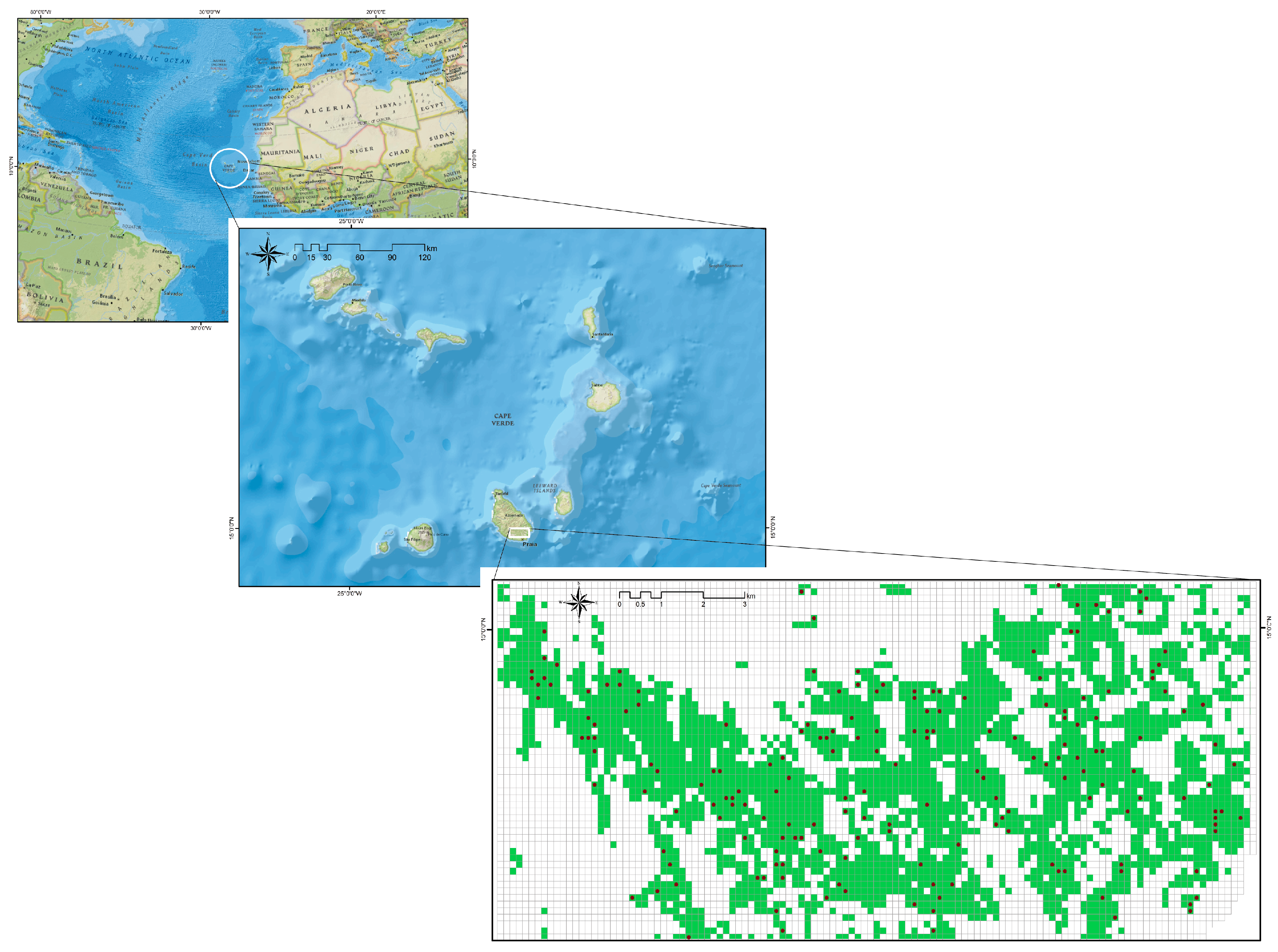
2.1.1. Study Area

Cape Verde is an archipelago of ten islands (nine inhabited) and five islets located in the eastern Atlantic Ocean, approximately 570 km from the coast of Senegal, West Africa (16°N, 24°W) (Figure 1).

The total land area for the archipelago is 4564 km². Cape Verde’s flora consists of 621 species of which 240 are indigenous and 84 endemic [26]. The current vegetation is the result of significant human impact that led to the introduction of nearly two thirds of the current species and substantial changes in the ecosystems. The Cape Verdean forests are the result of afforestation programs created over the past decades. The first afforestation programs initiated since 1930 during the Portuguese colonization. First in the humid areas and then intensified, after the country’s independence in 1975, in the arid and semi-arid zones to control soil erosion, and increasing the fuelwood and fodder production.

The study area is located in the south sector of Santiago Island, coordinates upper left 15°0′33.368′′N; 23°37′42.82′′W—lower right 14°56′11.818′′N; 23°27′40.946′′W, covering an area of 14,399 ha in the arid and semi-arid zones representatives of xerophytics woodlands of the island. Approximately 44% of this area is covered by forests (Figure 1) which are dominated by shrub-like growing species having an average canopy cover of 43%, and the mean tree density is 252 trees·ha⁻¹. Prosopis sp. represents the 95% in frequency, of the total fifteen wood species observed. Other species with some noticeable participation are Jatropha curcas, Acacia nilotica, Acacia Senegal, Parkinsonia aculeata and Acacia albida. The remaining non-forested land includes non-productive areas, agriculture and urban areas.

2.1.2. Field Data

The data used as ground truth for the study are based on the fieldwork carried out during the Cape Verde National Forest Inventory (NFI) in 2009. The inventory is based on a systematic sampling design with quadrats of 150 m. In the first phase of the NFI, the quadrats were classified in forest or non-forest by manual interpretation of high-resolution aerial orthophotography. The FAO forest definition was adopted. In the study area the forest area resulted in 14,399 ha.

In the second phase of the NFI, a subset of 10% of first phase forest units was selected by simple random sampling without replacement (SRSWOR) and surveyed in the field (Figure 1). In the center of each square a circular plot of 500 m² was created for such a purpose and all the trees in the plots taller than 50 cm were mapped and measured. The data collected are the following: tree position, tree species, tree height, crown projected area (based on 4 perpendiculars radius). The field work was carried out using the Field Map system [27]. For each field plot the AGB was calculated on the basis of local allometric equations developed within the CV-NFI [28]. The study on biomass models used destructive sampling of Prosopis juliflora that was carried out on three islands, namely Santo Antão, Santiago and Maio. The data used in this study are from 184 plots and 2218 measured trees.

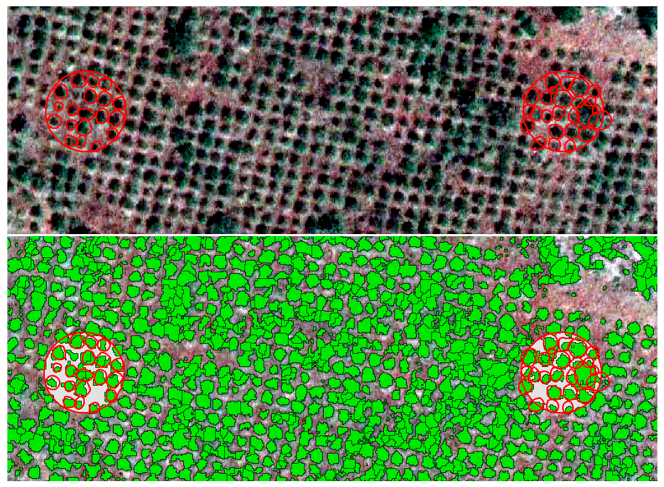
2.1.3. Aerial photo

The imagery dataset used for this study is an aerial RGB orthophoto acquired in January 2010 with a spatial resolution of 40 cm (

Table 1. The characteristic of the imagery used in the study.

Radiometric and Spectral Resolution	Natural Colour (RGB) 24-Bit Colour (3 × 8 Bits Per Band) Red, Blue, Green
Horizontal accuracies	±3 pixels
Sensor information	Analogic camera
Image width, height (pixels)	100,000 × 125,000
Ground sample distance (GSD)	0.4 × 0.4 m
Sun angle	>40°
Fly altitude	3800 m
Source	Geodata Air S.A.

).

The visible atmospherically resistant index (VARI) [29] in the form:

VARI = (Green − Red)/(Green + Red − Blue)

was calculated at this step and used as an additional band in the analysis.

2.1.4. Forest Map

When producing a wall-to-wall estimation of AGB it is essential to clearly define the spatial domain for which the estimation will be produced. Using the terminology adopted for the well-known k-nearest neighbors technique, such domain is called the target set which is the population units for which predictions of response variables (AGB biomass) are desired [30,31]. In this study we adopted as target set the forest area created in the first phase of the CV-NFI. From the original resolution of 150 m the forest/non-forest map was resampled at 22.4 m to approximately match the dimension (500 m²) of the field plots adopted in the NFI. This resulted in a total target set of 287,980 pixels corresponding to approximately 14,399 ha, for which the AGB estimation was produced.

2.2. Methods

In this study, we compared two approaches for the wall-to-wall prediction of AGB: (i) single tree detection, and (ii) area-based mapping. The first one is based on the object-oriented single tree mapping by image segmentation and object-oriented classification, while the second one is based on the pixel level tree crown mapping by unsupervised classification of the aerial imagery. Both the methods bring to the production of a plot level value of the crown projection area (CPA), which is then used as a predictor for the AGB estimation. We first present the methods used for both the approaches based on an empiric optimization of the algorithms, and then the final wall-to-wall estimation procedure.

2.2.1. Single Tree

The aerial image was processed by a multiresolution segmentation based on the well-known region growing algorithm implemented in the eCognition software [32]. After testing different settings combinations, we adopted a scale factor equal to 5, a color/shape ratio equal to 0.3, and a smoothness/compactness ratio equal to 0.6 (Figure 2).

2.2.2. Area-Based

After testing several supervised classification methods with both parametric and non-parametric approaches, we adopted an unsupervised classification based on the iso-clustering algorithm implemented in the TerrSet software [33,34].

Iso-clustering is an iterative self-organizing, unsupervised classifier based on a concept similar to the well-known isodata routine of Ball and Hall [35] and cluster routines such as the H-means and K-means procedures. We find that the best results were obtained using 8 clusters that were further reclassified to obtain a boolean map at 0.4 m resolution (Figure 3).

We then calculated the total CPA per each field plot as the area of the 0.4 m pixels from the boolean map for each one of the field plots of the NFI. We used a generalized linear model (GLM) to predict the total ABG biomass per plot on the basis of the CPA value.

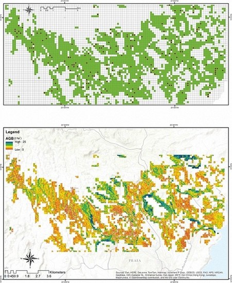
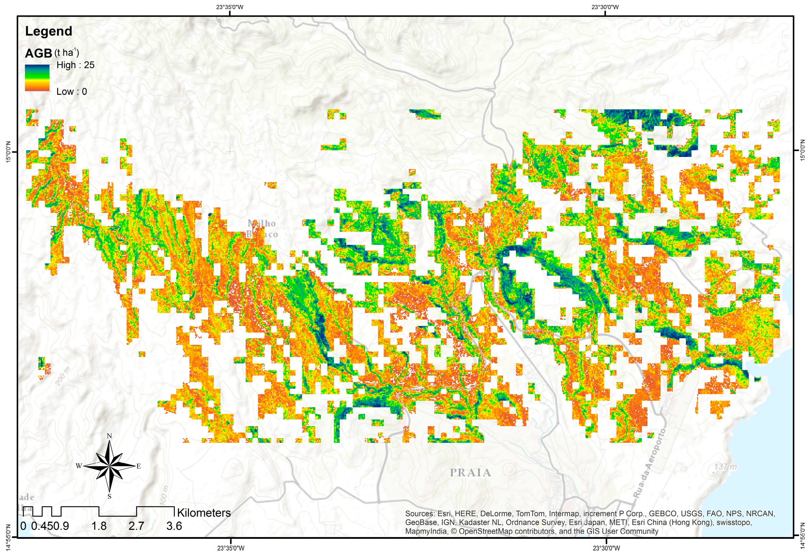
2.2.3. Wall-to-Wall AGB Spatial Estimation

For each of the 500 m² pixels in the 14,399 ha of forest in the study area, we calculated the CPA on the basis of the best model. This means that using the area-based approach we calculated the CPA summing up the 0.4 m resolution pixels from the boolean map. We then applied the linear model to derive a wall-to-wall estimation of the ABG biomass to all the 287,980 pixels of the target set.

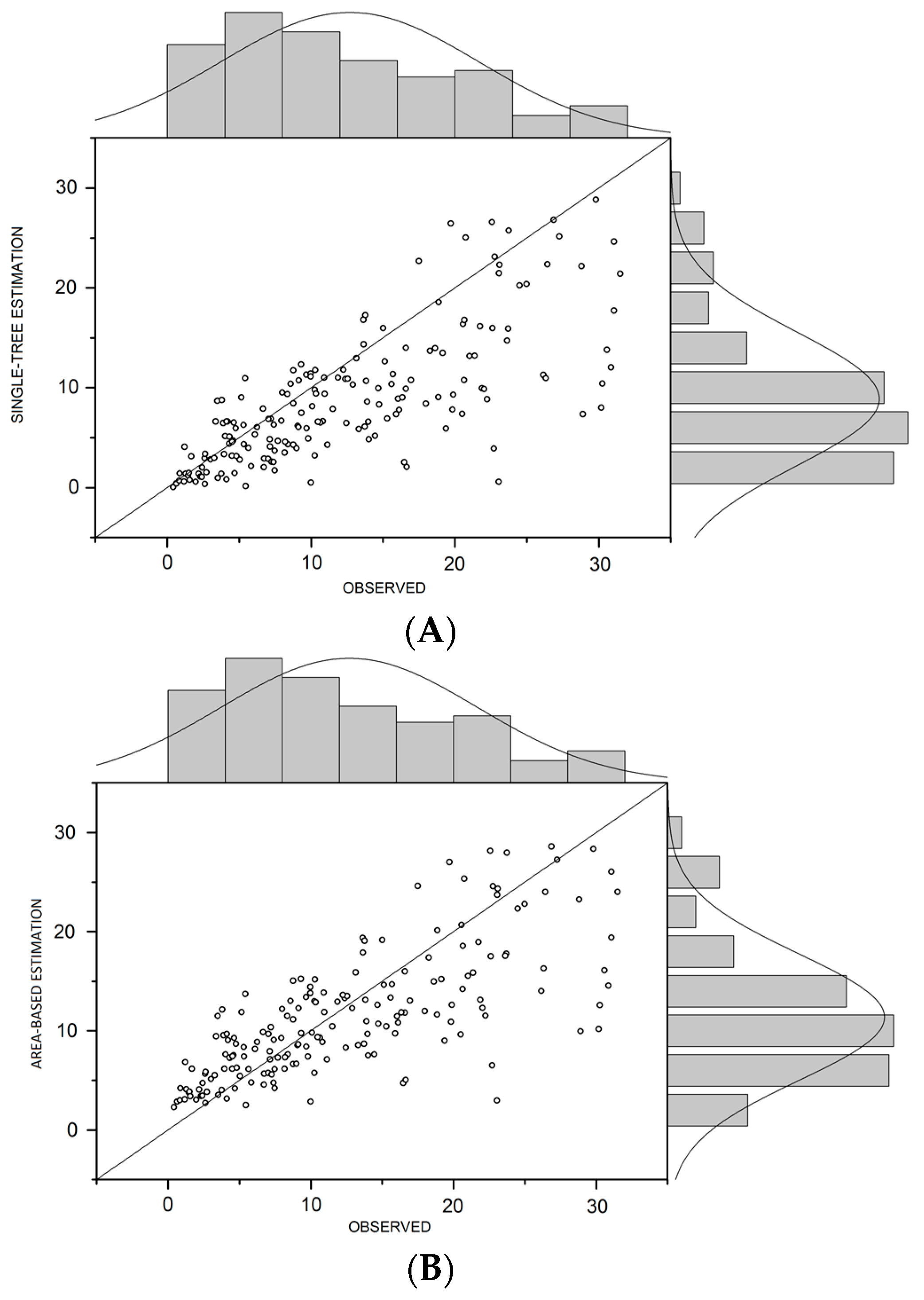
The accuracy of the final results was derived comparing estimates with measured AGB in the field by calculating the root mean square error (RMSE) (Equation (1)) and its percent version (RMSE%) (Equation (2)).

$$RMSE=\sqrt{\frac{{\displaystyle {\sum }_{i=1}^n{(X_{obs,i}-X_{model,i})}^2}}{n}}$$

(1)

$$RMSE\%=\frac{RMSE}{\overline{X_{obs}}}$$

(2)

where $X_{obs\text{},i}$ is the AGB measured in the i-th sampling unit and $X_{model,i}$ is the AGB estimated for the same i-th unit from the single-tree or area-based approach. $\overline{X_{obs}}$ is the average of the AGB measured in all the sampling units.

3. Results

The performance statistics of the linear models (Figure 4) developed for the single-tree and area-based approaches are in

Table 2. The parameters and performances of the GLM used to predict the AGB on the basis of CPA from the single-tree and area-based approach.

	Single-Tree		Area-Based
Intercept	131.79	SE = 29.69	−72.56	SE = 19.48
Slope	2.50	SE = 0.128	3.47	SE = 0.084
Pearson	0.83		0.95
Adj. R-Square	0.70		0.90

. Even if both the models demonstrated the possibility of predicting AGB (at the 0.05 level, the slope of the models was always significantly differ from zero), the area-based approach demonstrated better performances (Figure 4) with an adjusted R-square 30% higher than the tree-level result.

Wall-to-Wall Predictions

As expected from the model development phase, the area-based approach was able to produce a slightly more accurate spatial estimation of the AGB (RMSE of 4.76 t·ha⁻¹, 45% of the true average value) if compared with the tree-level approach (RMSE of 5.04 t·ha⁻¹, 48% of the true average value) (Figure 5).

The area-based model was used to derive the final AGB wall-to-wall spatial estimation in the study area (Figure 6).

4. Discussion

On the basis of the results achieved, both the models demonstrated a slight underestimation of the real AGB measured in the field, though the underestimation was higher for the single-tree approach (Figure 7).

From a visual inspection of the imagery, it seems that this phenomenon can be related to the fact that brighter crown portions of the trees tend to be confused with the soil background, resulting in an underestimation of the crown size mapped and thus of the predicted biomass. Moreover, the models cannot differentiate different values of biomass in those plots where the tree canopy occupies most of the plots area, in these conditions partial crown overlaps cannot be considered, resulting again in an underestimation of biomass predictions. This phenomenon, called saturation, is well documented in literature when biomass predictions are based on optical or radar images [36]. Sunlit and shaded area/ratio contain information that can further improve the predictions. In this study, they were not considered, but such information is essential to reveal vegetation clumping, and were found useful in spatial modeling of forest productivity [37,38].

The performance of our models is lower than what is reported in similar studies carried out on the basis of very high resolution multispectral satellite images. For example, Ozdemir [24] reports a RMSE of approximately 13% for the estimation of stem volume of sparse vegetation dominated by Juniperus spp. on the basis of QuickBird imagery in western Turkey. Several reasons can contribute to explaining these differences.

For example, in the single-tree approach we noticed that large crowns are sometimes segmented in more than one polygon that are thus erroneously considered as small trees with very little biomass. The biomass summed up at plot level of these artifacted small trees results much smaller than the real biomass. We tried to reduce this effect adjusting the scale of the segmentation process, but better results can be probably obtained by stratifying the image in subsets based on tree dimension and applying different segmentation scales in each subset.

Other uncertainty sources may have influenced the accuracy of the estimations, both on the basis of the single-tree or the area-based approach, but it was not possible to directly take into account all of them in this study.

For example, the relationship between data measured in the field plots and the analysis of the remotely sensed data are based on the perfect co-registration between the GNSS positioning acquired in the field and the georefering of the orthophotos. Errors in GNSS positioning cause observations of ground attributes to be associated with incorrect spectral values. This has an adverse impact on the possibility of deriving accurate spatially continuous maps and to draw correct inferences from them [39]. In this study, we tried to minimize this error source using real-time DGPS, electronic compass navigation and laser rangefinder. Nevertheless, the measurement of the tree crown projected area in the field is a challenging task for the irregularity and variability of crown shapes.

Finally, to reduce the bias of AGB pixel level estimation we recommend the use of predictions aggregated for larger areas. This type of approach is frequently recalled as small area estimation (SAE) [40]. For example, when the results are aggregated for the whole area of 14,399 ha the design-based estimation of the total AGB based on the sampling design was 182,882 Mg against 163,861 Mg predicted by the area-based model and 147,993 Mg predicted by the single-tree model.

As is clearly reported in literature, more accurate results in AGB estimations can be reached only with the introduction of different remotely sensed predicting variables, such as multispectral images, or 3D information from ALS or photogrammetry [25,41].

5. Conclusions

The goal of this study was to evaluate if non-photogrammetric visible aerial imagery could be used for the wall-to-wall prediction of forest biomass in a study area located in the island of Santiago in Cape Verde, dominated by xerophytic vegetation. More specifically, we were interested in comparing the single-tree and the area-based approaches. To do so, we used the data from the local National Forest Inventory made of 184 plots in a study area of 14,399 ha.

The results we obtained bring us to the following main conclusions.

• Aerial photography in these specific forest conditions characterized by sparse trees can be used to produce wall-to-wall predictions of forest biomass independently of the approach followed. This is relevant especially for those areas where ALS or high resolution multispectral satellite data are not yet available. Predictions are valid until the tree canopy tends to close. In areas with a denser tree canopy, estimations based on optical data only tend to accumulate higher uncertainty.
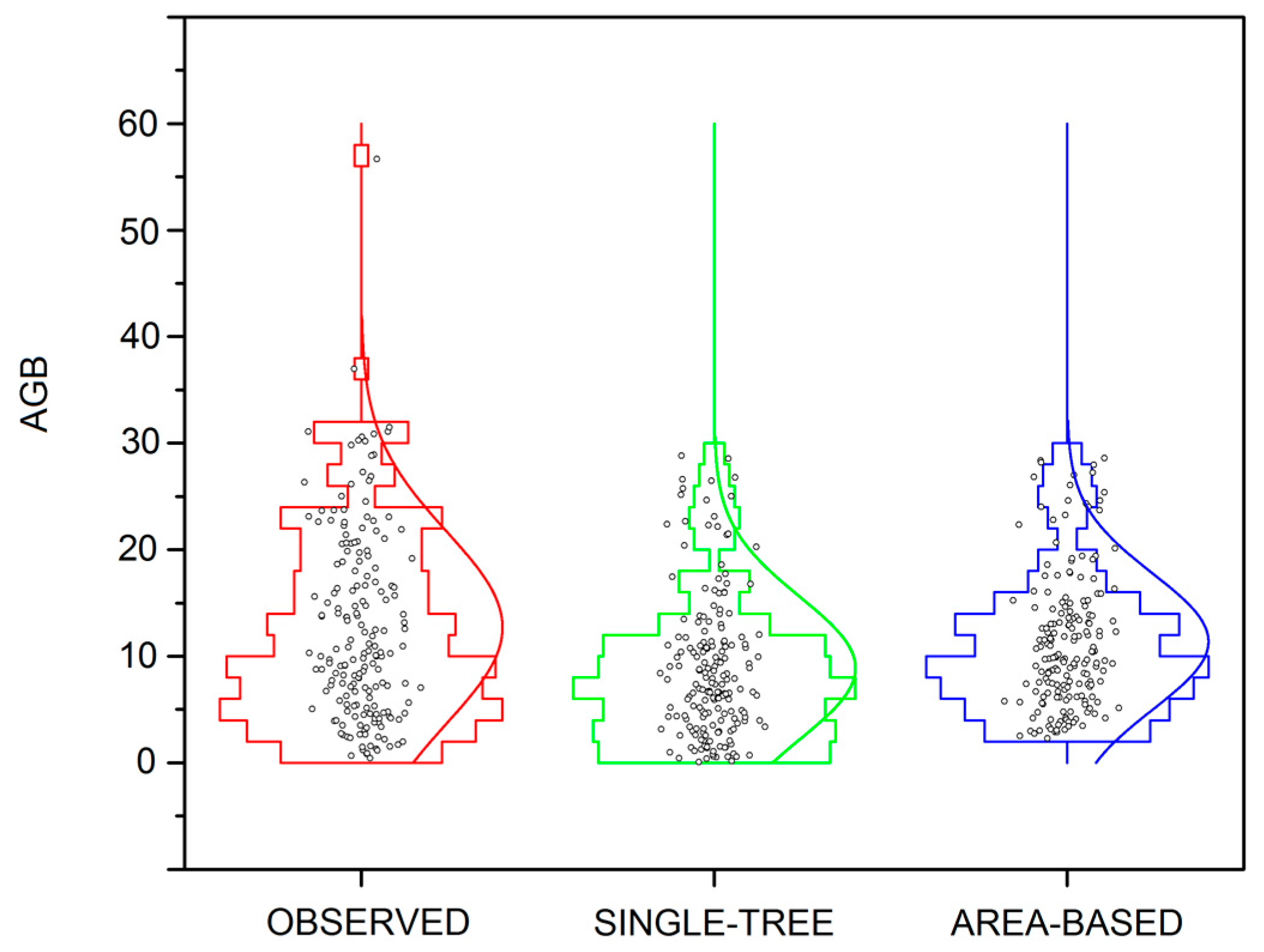
• The area-based approach was more accurate than the single-tree method. This is an important finding because this method is also the easiest in terms of image processing complexity and computation time and thus of hardware and software requirements. We noted that when the biomass values to be predicted are lower, the performance of the single-tree approach is higher, but the area-based approach demonstrates a more uniform prediction across the overall biomass range.

A further improvement of the method requires the stratification of the remotely sensed data on the basis of background characteristics and ancillary data, thus permitting a finer tuning during image processing.

Deeper GIS analysis oriented to the elaboration of more detailed forest maps can play a significant role in improving the estimation accuracy. This could be the basis for an iterative process of tuning the models for biomass and forest cover mapping that could be extended to the whole country.

References

- Foody, G.M. Remote sensing of tropical forest environments: Towards the monitoring of environmental resources for sustainable development. Int. J. Remote Sens. 2003, 24, 4035–4046. [Google Scholar] [CrossRef]
- Kumar, L.; Sinha, P.; Taylor, S.; Alqurashi, A.F. Review of the use of remote sensing for biomass estimation to support renewable energy generation. J. Appl. Remote Sens. 2015, 9, 097696_1–097696_28. [Google Scholar] [CrossRef]
- Klinge, H.; Rodriguez, W.A.; Brunig, E.; Fittkau, E.J. Biomass and structure in a central amazônian rain forest. In Tropical Ecological Systems: Trends in Terrestrial and Aquatic Research; Golley, F.B., Medina, E., Eds.; Springer: Berlin, Germany, 1975; pp. 115–122. [Google Scholar]
- Overman, J.P.M.; Witte, H.J.L.; Saldarriaga, J.G. Evaluation of regression models for above-ground biomass determination in Amazon rainforest. J. Trop. Ecol. 1994, 10, 207–218. [Google Scholar] [CrossRef]
- Nelson, B.W.; Mesquita, R.; Pereira, J.L.G.; de Souza, S.G.A.; Batista, G.T.; Couto, L.B. Allometric Regression for Improved Estimate of Secondary Forest Biomass in the Central Amazon. For. Ecol. Manag. 1999, 117, 149–167. [Google Scholar] [CrossRef]
- Henry, M.; Besnard, A.; Asante, W.A.; Eshun, J.; Adu-Bredu, S.; Valentini, R.; Bernoux, M.; Saint-André, L. Wood density, phytomass variations within and among trees, and allometric equations in a tropical rainforest of Africa. For. Ecol. Manag. 2010, 260, 1375–1388. [Google Scholar] [CrossRef]
- Chave, J.; Réjou-Méchain, M.; Búrquez, A.; Chidumayo, E.; Colgan, M.S.; Delitti, W.B.C.; Duque, A. Improved allometric models to estimate the aboveground biomass of tropical trees. Glob. Chang. Biol. 2014, 20, 3177–3190. [Google Scholar] [CrossRef] [PubMed]
- Brown, S.; Lugo, A.E. Biomass of tropical forests: A new estimate based on forest volume. Science 1984, 223, 1290–1293. [Google Scholar] [CrossRef] [PubMed]
- Lehtonen, A.; Mäkipää, R.; Heikkinen, J.; Sievänen, R.; Liski, J. Biomass expansion factors (BEFs) for scots pine, Norway spruce and birch according to stand age for boreal forests. For. Ecol. Manag. 2004, 188, 211–224. [Google Scholar] [CrossRef]
- Segura, M.; Kanninen, M. Allometric models for tree volume and total aboveground biomass in a tropical humid forest in costa rica. Biotropica 2005, 37, 2–8. [Google Scholar] [CrossRef]
- Smyth, C.; Kurz, W.; Neilson, E.; Stinson, G. National-scale estimates of forest root biomass carbon stocks and associated carbon fluxes in Canada. Glob. Biogeochem. Cycles 2013, 27, 1262–1273. [Google Scholar] [CrossRef]
- Rivington, M.; Matthews, K.B.; Bellocchi, G.; Buchan, K. Evaluating uncertainty introduced to process-based simulation model estimates by alternative sources of meteorological data. Agric. Syst. 2006, 88, 451–471. [Google Scholar] [CrossRef]
- Zhang, L.; Yu, G.; Gu, F.; He, H.; Zhang, L.M.; Han, S. Uncertainty Analysis of Modeled Carbon Fluxes for a Broad-leaved Korean Pine Mixed Forest Using a Process-based Ecosystem Model. J. For. Res. 2012, 17, 268–282. [Google Scholar] [CrossRef]
- Lu, D.; Chen, Q.; Wang, G.; Liu, L.; Li, G.; Moran, E. A survey of remote sensing-based aboveground biomass estimation methods in forest ecosystems. Int. J. Digit. Earth 2014. [Google Scholar] [CrossRef]
- Wang, Q.; Adiku, S.; Tenhunen, J.; Granier, A. On the relationship of NDVI with leaf area index in a deciduous forest site. Remote Sens. Environ. 2005, 94, 244–255. [Google Scholar] [CrossRef]
- Leckie, D.G. Advances in remote sensing technologies for forest surveys and management. Can. J. For. Res. 1990, 20, 464–483. [Google Scholar] [CrossRef]
- Greer, J.D. The view from above. J. For. 1993, 8, 10–14. [Google Scholar]
- Holopainen, M.; Lukkarinen, E. Digital Aerial Photographs in Forest Inventory; Department of Forest Resource Management Publications, University of Helsinki: Helsinki, Finland, 1994; Volume 4, pp. 1–33. [Google Scholar]
- Blackburn, G.A.; Milton, E.J. An ecological survey of deciduous woodlands using airborne remote sensing and geographical information systems (GIS). Int. J. Remote Sens. 1997, 18, 1919–1935. [Google Scholar] [CrossRef]
- Tuominen, S.; Haapanen, R. Estimation of forest biomass by means of genetic algorithmbased optimization of airborne laser scanning and digital aerial photograph features. Silva Fenn. 2013, 47, 902. [Google Scholar] [CrossRef]
- Uuttera, J.; Haara, A.; Tokola, T.; Maltamo, M. Determination of the spatial distribution of trees from digital aerial photographs. For. Ecol. Manag. 1998, 110, 275–282. [Google Scholar] [CrossRef]
- Gärtner, P.; Förster, M.; Kurbanb, A.; Kleinschmit, B. Object based change detection of Central Asian Tugai vegetation with very high spatial resolution satellite imagery. Int. J. Appl. Earth Obs. Geoinf. 2014, 31, 110–121. [Google Scholar] [CrossRef]
- Ardila, J.P.; Bijker, W.; Tolpekin, V.A.; Stein, A. Quantification of crown changes and change uncertainty of trees in an urban environment. ISPRS J. Photogram. Remote Sens. 2012, 74, 41–55. [Google Scholar] [CrossRef]
- Ozdemir, I. Estimating stem volume by tree crown area and tree shadow area extracted from pan-sharpened Quickbird imagery in open Crimean juniper forests. Int. J. Remote Sens. 2008, 29, 5643–5655. [Google Scholar] [CrossRef]
- Hirschmugl, M.; Ofner, M.; Raggam, J.; Schardt, M. Single tree detection in very high resolution remote sensing data. Remote Sens. Environ. 2007, 110, 533–544. [Google Scholar] [CrossRef]
- Brochmann, C.; Rustan, Ø.H.; Lobin, W.; Kilian, N. The Endemic Vascular Plants of the Cape Verde Islands, W Africa (Sommerfeltia); Botanical Garden and Museum, University of Oslo: Oslo, Norway, 1997; Volume 24, pp. 1–356. [Google Scholar]
- Černý, M.; Bukša, I.F.; Pasternak, V.P. Usage of Field Technology Field-Map in Forest Management and Nature Protection; Geoinformatics: Kiev, Ukraine, 2006. [Google Scholar]
- Cienciala, E.; Centeio, A.; Blazek, P.; Soares, M.C.G.; Russ, R. Estimation of stem and tree level biomass models for Prosopis juliflora/pallid applicable to multi-stemmed tree species. Trees 2013, 27, 1061–1070. [Google Scholar] [CrossRef]
- Gitelson, A.A.; Kaufman, Y.J.; Stark, R.; Rundquist, D. Novel algorithms for remote estimation of vegetation fraction. Remote Sens. Environ. 2002, 80, 76–87. [Google Scholar] [CrossRef]
- Chirici, G.; Barbati, A.; Corona, P.; Marchetti, M.; Travaglini, D.; Maselli, F.; Bertini, R. Non-parametric and parametric methods using satellite images for estimating growing stock volume in alpine and Mediterranean forest ecosystems. Remote Sens. Environ. 2008, 112, 2686–2700. [Google Scholar] [CrossRef]
- Chirici, G.; Mura, M.; McInerney, D.; Py, N.; Tomppo, E.O.; Waser, L.T.; Travaglini, D.; McRoberts, R.E. A meta-analysis and review of the literature on the k-Nearest Neighbors technique for forestry applications that use remotely sensed data. Remote Sens. Environ. 2016, 176, 282–294. [Google Scholar] [CrossRef]
- Mueller, M.; Segl, K.; Kaufmann, H. Edge-and region-based segmentation technique for the extraction of large, man-made objects in high-resolution satellite imagery. Pattern Recognit. 2004, 37, 1619–1628. [Google Scholar] [CrossRef]
- Adams, R.; Bischof, L. Seeded region growing. IEEE Trans. Pattern Anal. Mach. Intell. 1994, 16, 641–647. [Google Scholar] [CrossRef]
- Shih, F.Y.; Cheng, S. Automatic seeded region growing for color image segmentation. Image Vis. Comput. 2005, 23, 877–886. [Google Scholar] [CrossRef]
- Ball, G.H.; Hall, D.J. A Novel Method of Data Analysis and Pattern Classification; Stanford Research Institute: Menlo Park, CA, USA, 1965. [Google Scholar]
- Wang, G.; Zhang, M.; Gertner, G.Z.; Oyana, T.; McRoberts, R.E.; Ge, H. Uncertainties of Mapping Aboveground Forest Carbon Due to Plot Locations Using National Forest Inventory Plot and Remotely Sensed Data. Scand. J. For. Res. 2011, 26, 360–373. [Google Scholar] [CrossRef]
- Chen, J.M.; Menges, C.H.; Leblanc, S.G. Global mapping of foliage clumping index using multi-angular satellite data. Remote Sens. Environ. 2005, 97, 447–457. [Google Scholar] [CrossRef]
- He, L.; Chen, J.; Pisek, J.; Strahler, A.H. Global clumping index map derived from the MODIS BRDF product. Remote Sens. Environ. 2012, 119, 118–130. [Google Scholar] [CrossRef]
- McRoberts, R.E. The effects of rectification and Global Positioning System errors on satellite image-based estimates of forest area. Remote Sens. Environ. 2010, 114, 1710–1717. [Google Scholar] [CrossRef]
- Breidenbach, J.; Astrup, R. Small area estimation of forest attributes in the Norwegian National Forest Inventory. Eur. J. For. Res. 2012, 131, 1255–1267. [Google Scholar] [CrossRef]
- Tuominen, S.; Pitkänen, J.; Balazs, A.; Korhonen, K.T.; Hyvönen, P.; Muinonen, E. NFI plots as complementary reference data in forest inventory based on airborne laser scanning and aerial photography in Finland. Silva Fenn. 2014, 48, 983. [Google Scholar] [CrossRef]