Abstract
Wind farms (WFs) can affect the local climate, and local climate change may influence underlying vegetation. Some studies have shown that WFs affect certain aspects of the regional climate, such as temperature and rainfall. However, there is still no evidence to demonstrate whether WFs can affect local vegetation growth, a significant part of the overall assessment of WF effects. In this research, based on the moderate-resolution imaging spectroradiometer (MODIS) vegetation index, productivity and other remote-sensing data from 2003 to 2014, the effects of WFs in the Bashang area of Northern China on vegetation growth and productivity in the summer (June–August) were analyzed. The results showed that: (1) WFs had a significant inhibiting effect on vegetation growth, as demonstrated by decreases in the leaf area index (LAI), the enhanced vegetation index (EVI), and the normalized difference vegetation index (NDVI) of approximately 14.5%, 14.8%, and 8.9%, respectively, in the 2003–2014 summers. There was also an inhibiting effect of 8.9% on summer gross primary production (GPP) and 4.0% on annual net primary production (NPP) coupled with WFs; and (2) the major impact factors might be the changes in temperature and soil moisture: WFs suppressed soil moisture and enhanced water stress in the study area. This research provides significant observational evidence that WFs can inhibit the growth and productivity of the underlying vegetation.
1. Introduction
Wind turbines can modify the surface fluxes of momentum, sensible heat, water vapor, and carbon dioxide by enhancing turbulence, increasing surface roughness, and changing the stability of the atmospheric boundary layer (ABL) [1,2]. As reported in previous studies, the large establishment of wind farms (WFs) influence the local climate [3,4]. Based on field campaigns or model simulations, these studies found that large-scale WFs could alter local temperature, reduce precipitation and even mitigate extreme weather [5,6,7]. However, due to lack of sufficient observations for validation and the simple parameterization of WFs, the simulated results have significant uncertainties [4,8]. In addition, field campaigns usually cover a short time span and include only a few measurements, limiting the representativeness of the results. Therefore, due to the limitations of climate models and field campaigns, an increasing number of studies are using remote-sensing data to investigate the effects of WFs on regional climate [9,10,11,12,13]. Remote sensing data provides global spatial sampling information with high temporal and spatial resolution, and can thus be used to analyze the effects of large-scale WFs. Zhou et al. analyzed the effects of WFs on land surface temperature (LST) in Texas and found a nighttime warming effect of 0.31 °C–0.70 °C [9,10]. Slawsky et al. analyzed the impacts of three WFs in Northern Illinois and provided further observational evidence of a warming effect at night caused by WFs [14].
Since wind farms can affect local climate [9,12,15], changes in local climate, such as temperature and precipitation, may affect local vegetation growth and productivity over WFs [16]. Since the beginning of the 21st century, China has built enormous wind turbines. In 2010, wind energy capacity in China reached 42.3 GW, exceeding the 40.3 GW capacity of the United States, and ranking first in the world. In 2015, newly-installed wind energy capacity in China amounted to 30.8 GW, accounting for 48.9% of newly-installed capacity worldwide [17]. Within this newly installed wind energy capacity, wind energy development has been fastest in Hebei province and Inner Mongolia [18,19]. However, the effects of the rapid development of WFs on local climate and vegetation growth in China have not yet been thoroughly evaluated.
In this paper, we use the moderate-resolution imaging spectroradiometer (MODIS) vegetation index (leaf area index, LAI; normalized difference vegetation index, NDVI; and enhanced vegetation index, EVI) data, MODIS productivity data (gross primary production, GPP; net primary production, NPP), and other auxiliary data (temperature, soil moisture, evapotranspiration, albedo, and wind) to analyze the effects of WFs on summer (June–August, JJA) vegetation growth in the Bashang area of Northern China. The specific objectives of this paper are as follows: (1) to identify whether the WFs in Bashang can influence the summer vegetation growing status and productivity and (2) to further explore the possible processes for the effects of WFs on local vegetation growth.
2. Materials and Methods
2.1. Study Area
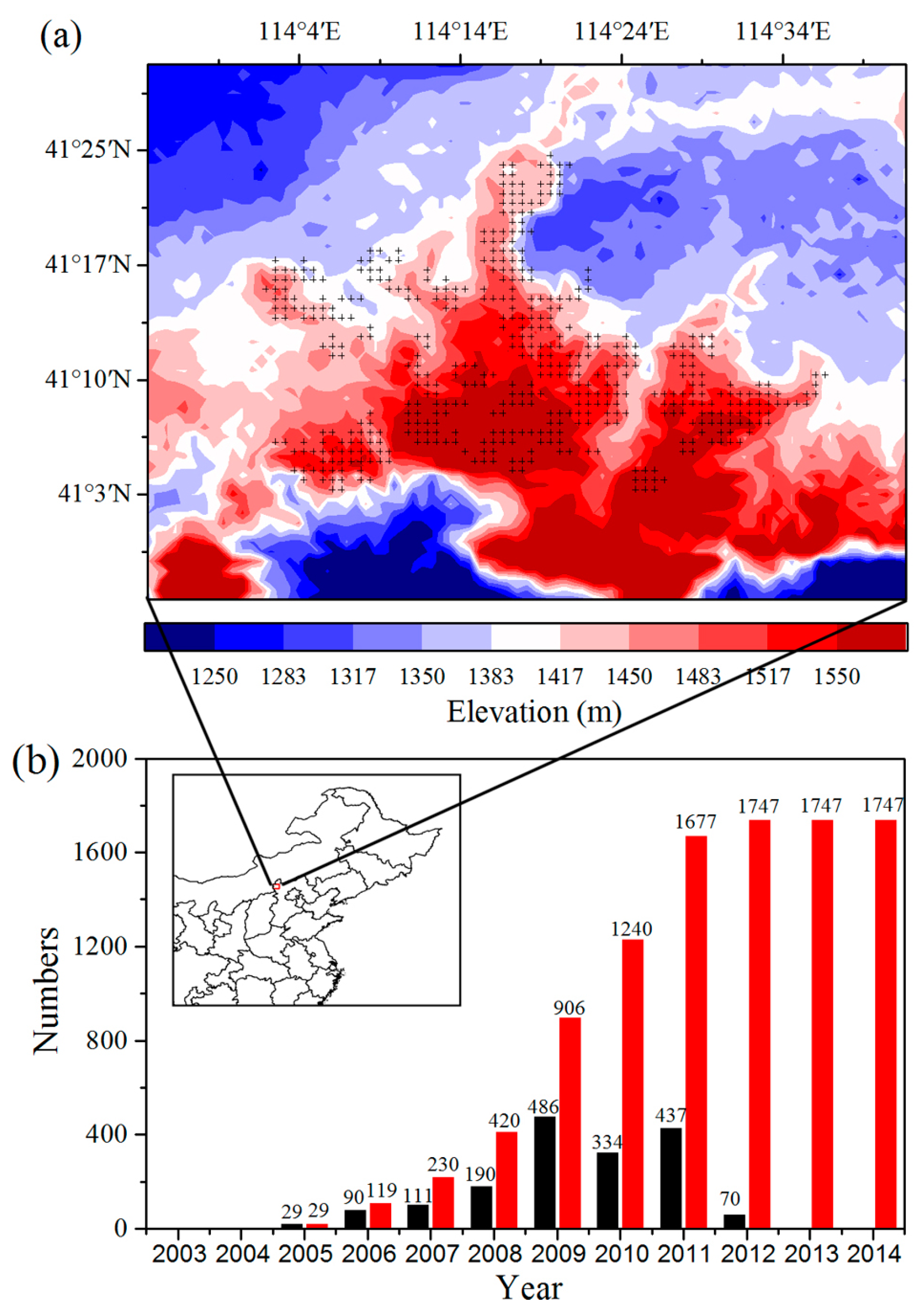
The study area (40.9°N–41.5°N, 113.9°E–114.7°E) is located in the Bashang area of Hebei province, Northern China (Figure 1a). In 2005, WF construction began in the study area and was completed near the end of 2011. We verified the wind turbines on Google Earth and confirmed the locations of a total of 1747 wind turbines in the study area by field campaigns (Figure 1b). The heights of the wind turbines range from 77 m to 93 m, and the diameters of their support columns are nearly 4 m. The land cover types in the study area consist mainly of crops, grassland, water, wetlands, and urban areas. The major land cover types of the regions where the WFs are located are crops and grassland, accounting for 44.7% and 53.4%, respectively, of the land cover (Figure S1).
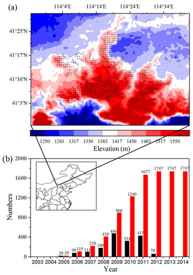
Figure 1.
(a) Surface elevation (m) at ~1 km spatial resolution for the study region. Plus symbols represent pixels with one or more wind turbines. (b) Number of individual wind turbines built annually over the period 2003–2014. The numbers of annual (black) and accumulated (red) turbines built for each year are shown on the top of the bar. The location of the study region is plotted within the map of northeast China. The data is based on “2012–2015 Research Report of China wind power market and being built in the construction of wind farm project.” The location of study area is plotted (red) within the map of China.
2.2. Data
The vegetation indexes (VIs) in this paper are from the Collection 5 MODIS 8-days, and 1 km leaf area index (LAI) data (MOD15A2) for the period 2003–2014. The monthly normalized difference vegetation index (NDVI) and enhanced vegetation index (EVI) data (MOD13A3) with a spatial resolution of 1 km are also used to characterize vegetation growth status [20]. The vegetation productivity data used in this paper include gross (GPP, MOD17A2) and net primary productivity (NPP, MOD17A3) with a spatial resolution of 1 km. The temporal resolution of GPP and NPP are eight days and one year, respectively [21,22]. Since there is no suitable monthly NPP data, annual NPP data was used to characterize the changes in the net primary production of vegetation.
To investigate the processes of the observed effects, we use related auxiliary data, including the MODIS LST, albedo and evapotranspiration (ET), Climate Change Initiative (CCI) soil moisture v02.2 and wind speed and direction of Modern-Era Retrospective Analysis for Research and Applications (MERRA) [23]. The temporal and spatial resolution of the LST (MYD11A2), albedo (MCD43B3) and ET (MOD16A2) are every eight-days and 1 km [24,25,26], respectively, and those of the soil moisture data are daily and 0.25° [27]. The LST product for Aqua (MYD11A2) includes two measurements, at approximate local solar times of 13:30 and 01:30. The wind speed and direction of MERRA are composites of the U- and V-wind speeds, with a temporal resolution of once per hour and a spatial resolution of 0.5° × 0.667° [23]. In this research, the wind speeds and directions at 50 m above the surface at 05:30 and 17:30 (UTC), which approximately correspond to the local times of 13:30 and 01:30 in the study area, are chosen. Since this height is close to the height of the wind turbines, it can approximately represent the wind speeds associated with the wind turbines.
2.3. Data Processing and Methods
The MODIS data used in this paper are all the sinusoidal equal-area projections of 1 km and then re-projected onto a 0.01° resolution, which are coarser than the 1 km data to avoid spatial gaps [14]. Finally, there are 4617 pixels (81 columns, 57 rows), covering 1747 wind turbines. Vegetation growth exhibits strong spatial variability at the pixel level, which is mostly related to changes in topography or land surface types. Although the EVI varies from one wind farm to another, and between WFPs and NNWFPs, the mean areal EVI difference between WFPs and NNWFPs is very small (Figure S2). The effects of surface heterogeneity, such as land surface type and topography, are minimized by using average anomalies [11]. First, the average summer (June–August) average values of LAI and GPP for every year are calculated, and are then used to create summer anomalies by subtracting the climatological data at every pixel during 2003–2014. The NPP, LST, albedo, and ET data are processed in the same way. According to the longitudes and latitudes of the wind turbines’ locations, the corresponding pixels for the soil moisture data are chosen. The summer averages and the anomalies of soil moisture are then calculated.
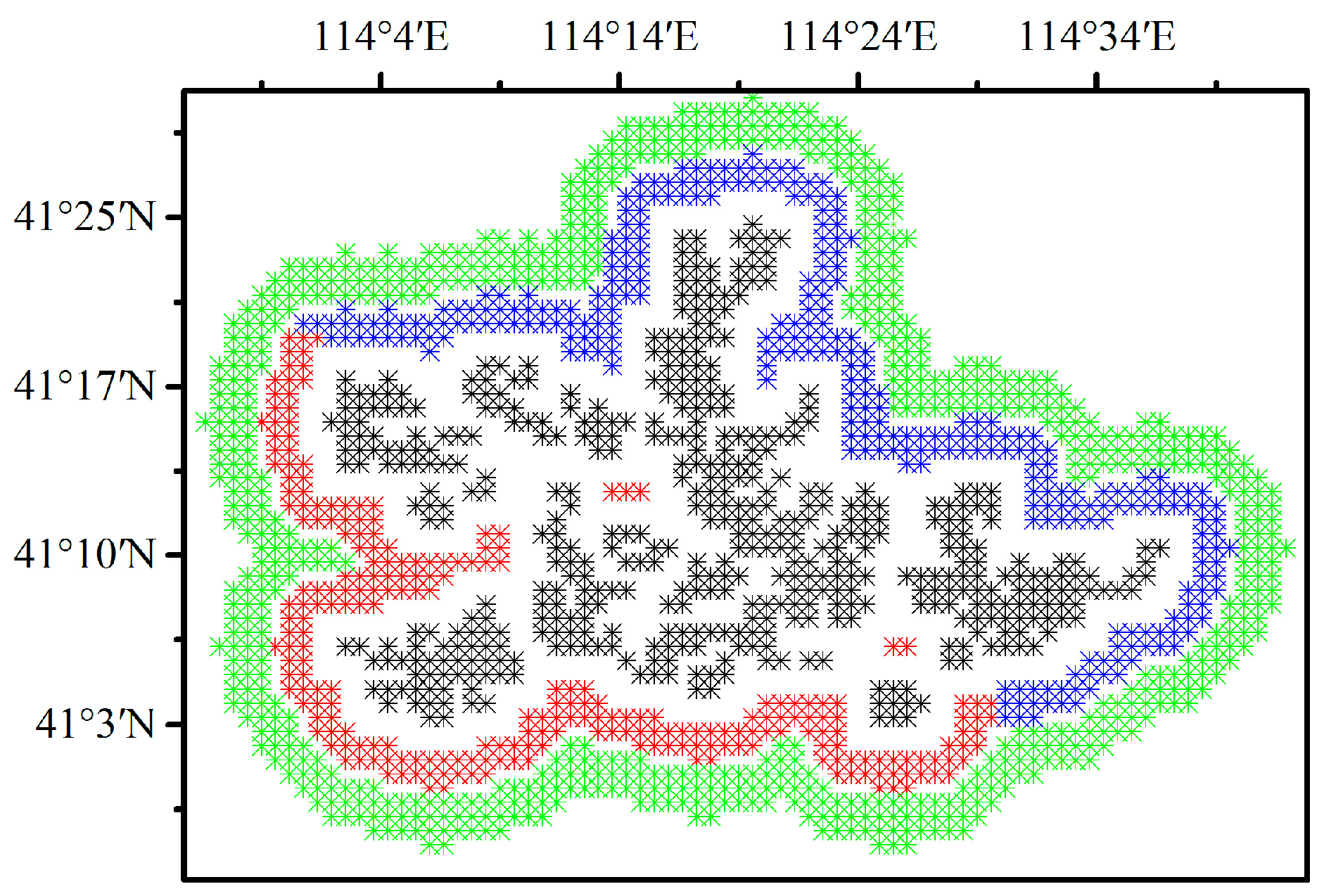
Pixels containing at least one wind turbine are defined as wind farm pixels (WFPs) and pixels located 6 to 9 km away from the WFPs are defined as nearby non-wind-farm pixels (NNWFPs) [9,28]. The transitional zone between WFPs and NNWFPs avoids the effect of turbulence caused by blade rotation on the NNWFPs [29]. Finally, a total of 484 WFPs and 690 NNWFPs are obtained (Figure 2). To explore the downwind effect of the WFs, the 537 pixels that are 3 to 5 km away from the WFPs are divided into the following two groups: upwind wind farm pixels (UWFPs, 245 pixels) and downwind wind farm pixels (DWFPs, 292 pixels) (Figure 2). Since the wind direction in the study area during the growing season is mainly from the southwest to northeast (see the discussion), the pixels to the southwest of WFPs are designated as UWFPs, and the pixels to the northeast of WFPs are designated as DWFPs.
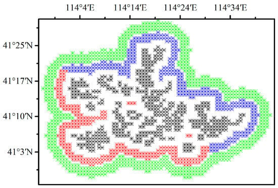
Figure 2.
Definition of wind farm pixels (WFPs, 484 pixels in black), upwind wind farm pixels (UWFPs, 245 pixels in red), downwind wind farm pixels (DWFPs, 292 pixels in blue) and nearby non-wind farm pixels (NNWFPs, 690 pixels in green) at a spatial resolution of 0.01°.
As the background LAI varies substantially from one year to another, in order to highlight the spatial variability at the pixel scale, for each year the regional mean LAI anomalies (one constant value) are removed from the original anomalies as proposed by Zhou et al. [9]. Then, the differences of average LAI anomalies, during the post- and pre-turbine construction periods, are calculated to analyze the spatial coupling between the differences and the layout of wind turbines. Since the wind turbines built during 2006–2011 in the study area account for 94.3% of the total, two time periods are selected to represent pre- and post-turbine construction periods, 2003–2005 and 2012–2014. In addition, two single years, 2004 and 2012 (the regional mean anomalies are similar), are chosen to calculate the differences in the LAI anomaly for two individual years. Note that the LAI changes shown in the figures represent changes relative to regional mean values rather than absolute changes. The study area is very small (0.6° × 0.8°) and, therefore, it can be reasonably assumed that the WFPs and NNWFPs have the same climatic background. If the development of wind turbines can affect the LAI, the LAI difference between WFPs and NNWFPs will change over time. The effects of the WFs on vegetation growth are quantified by using the average LAI difference between WFPs and NNWFPs (WFPs minus NNWFPs) after the building of the WFs (2012–2014) subtracted from that before building the WFs (2003–2005). The calculation of GPP and NPP anomalies differences follow a similar approach.
In this research, the SCI (spatial coupling index) is used to assess the spatial coupling of the wind turbines pattern with LAI changes [14]. The differences of 4617 LAI in the study area are ranked in decreasing order, and the first 5% (231), 10% (462), and 15% (693) of pixels with the smallest LAI differences (the strongest decreasing signal) are selected. Then, the percentage of these 5%, 10%, and 15% pixels falling into the WFPs (484 pixels), NNWFPS (690 pixels), UWFPs (245 pixels), and DWFPs (292 pixels) are calculated and referred to as SCI. For example, if there are 100 pixels in the top 10% pixels (462) with the smallest LAI differences falling into WFPs, the SCI of WFPs is 21.6% (100 pixels divided by 462 pixels). If the LAI changes are distributed randomly, the possibilities of the four groups (referred to as the threshold of SCI) would have been 10.5% (484 pixels divided by 4617 pixels) for WFPs, 14.9% (690 pixels divided by 4617 pixels) for NNWFPs, 5.3% (245 pixels divided by 4617 pixels) for UWFPs, and 6.3% (292 pixels divided by 4617 pixels) for DWFPs. If the SCI is larger than the threshold of SCI, it means that the VI changes have a good spatial coupling with the group.
3. Results
First, the spatial coupling of the layout of WFPs and LAI anomaly differences are calculated to analyze the effect of the WFs on vegetation growth. Figure 3a–c show LAI anomaly differences at pixel scale in the summer between pre- and post-turbine construction periods (2012–2014 minus 2003–2005), and the probability distributions of LAI anomaly differences between WFPs and NNWFPs. The results show that negative LAI anomaly differences are spatially coupled with wind turbines, with 86.2% of WFPs corresponding to negative LAI anomaly differences. The average of LAI anomaly differences is −0.11 ± 0.10 and 0.01 ± 0.13 for WFPs and NNWFPs, a significant difference (p < 0.01) according to the t-test statistics. This result indicates that WFPs inhibit vegetation growth compared with NNWFPs. The spatial distributions of individual year average LAI anomaly differences are very similar to those of multi-year averages (Figure 3b,d), with 84.1% of WFPs corresponding to the negative LAI anomaly differences. The average of LAI anomaly differences is −0.12 ± 0.13 and 0.01 ± 0.13 for WFPs and NNWFPs, respectively, which is also a significant difference (p < 0.01). The anomaly differences for NDVI and EVI are also analyzed in this paper. The results for NDVI and EVI are found to be very similar to those for LAI, which indicates that the WFs inhibit vegetation growth in summer (Figure S3). Note that, to the northeast of the WFs, there is a small area with zero anomalies in the vegetation index and net vegetation productivity. The reason for this observation is that the land cover type in this area is a lake, and the MODIS LAI and the vegetation productivity present no data for this area.
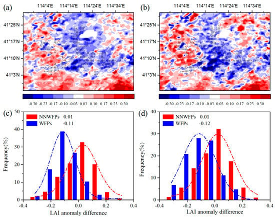
Figure 3.
Summer MODIS LAI anomaly differences and the corresponding LAI anomaly differences probability distribution of WFPs and NNWFPs between post- and pre-turbine-construction years (a,c) (2012–2014 minus 2003–2005 averages) and (b,d) (2012 minus 2004). WFPs and NNWFPs are defined as in Figure 2. Plus symbols represent pixels with one or more wind turbines.
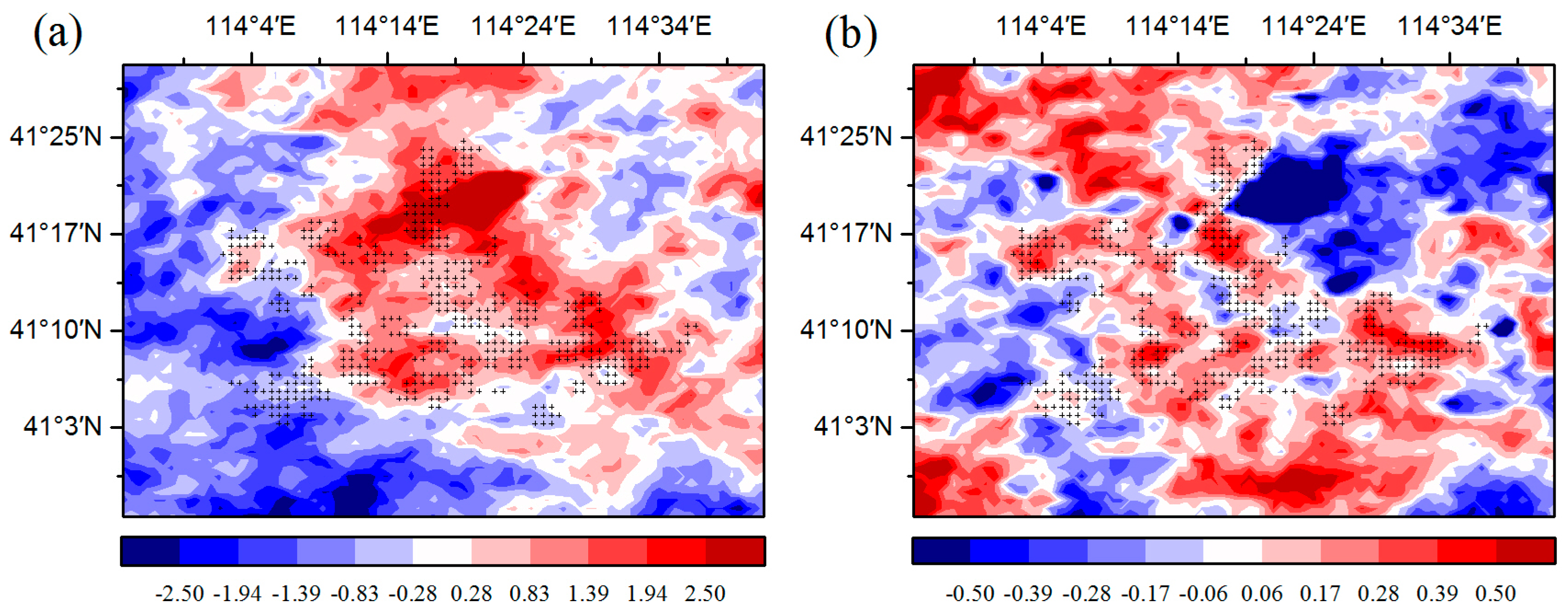
Then, the effects of WFs on vegetation productivity are analyzed. Figure 4 shows the summer GPP and annual NPP differences at pixel scale between the pre- and post-turbine construction periods (2012–2014 minus 2003–2005) in the study area. The results show that 80.4% negative summer GPP anomaly differences are spatially coupled with the wind turbines (Figure 4a). The average of GPP anomaly differences is −16.51 ± 21.10 (−0.42 ± 33.59) g C m−2 JJA−1 for WFPs (NNWFPs), which are significantly different (p < 0.01) according to the t-test statistics. The annual NPP anomaly differences over WFPs (−8.36 ± 13.08 g C m−2 year−1) are significantly smaller than that over NNWFPs (0.19 ± 19.02 g C m−2 year−1, p < 0.01), with 71.9% of WFPs corresponding to negative NPP anomaly differences (Figure 4b). We also calculated average summer GPP and annual NPP of WFPs and NNWFPs in 2003–2005 and 2012–2014 (Figure 4c,d). From 2003 to 2005, the average summer GPP over WFPs is 179.03 g C m−2 JJA−1 and significantly larger than the GPP (175.26 g C m−2 JJA−1) over NNWFPs (p < 0.01). From 2012 to 2014, the average summer GPP over WFPs (NNWFPs) increased to 291.78 (304.10 g C m−2 JJA−1). Vegetation productivity in WFPs has a smaller rate of increase in summer GPP, becoming significantly smaller than that in NNWFPs (p < 0.01). From 2003 to 2005, the average annual NPP over WFPs (236.18 g C m−2 year−1) is significantly larger than that over NNWFPs (232.68 g C m−2 year−1, p < 0.05). From 2012 to 2014, the average annual NPP over WFPs (NNWFPs) decreased to 222.67 (227.72 g C m−2 year−1). Vegetation productivity in the WFPs has a larger rate of decrease of NPP, becoming significantly smaller than that in NNWFPs (p < 0.01). The results of summer GPP and annual NPP indicate that, compared with NNWFPs, WFPs inhibit vegetation productivity.
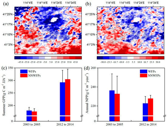
Figure 4.
(a) Summer MODIS GPP (g C m−2 JJA−1) and (b) annual MODIS NPP (g C m−2 year−1) anomaly differences between post- and pre-turbine construction years (2012–2014 minus 2003–2005 averages). (c) Average summer GPP and (d) annual NPP of WFPs and NNWFPs in 2003–2005 and 2012–2014.
The spatial coupling of the layout of the WFPs and vegetation index and productivity anomaly differences, are quantified by comparing the SCI values of 5%, 10%, and 15% pixels of the smallest vegetation index as well as GPP, and NPP anomaly differences located in WFPs with the corresponding SCI threshold. Generally, the larger the SCI value, the stronger the spatial coupling. The SCI values for LAI, NDVI, EVI, GPP, and NPP in WFPs range from 9.5% to 35.5%, and 14 of the 15 are larger than the threshold (10.8%), indicating a strong spatial coupling between the layout of WFPs and vegetation anomaly differences. In other words, WFs can inhibit vegetation growth and productivity (Table 1).

Table 1.
Variations in the percentage of the top 5%, 10%, and 15% pixels with the strongest decreasing anomalies falling into each group of pixels (referred to as spatial coupling index (SCI)). WFPs, NNWFPs, DWFPs, and UWFPs are defined in the main text and are shown in Figure 2. Values with (*) are larger than those that would be generated randomly.
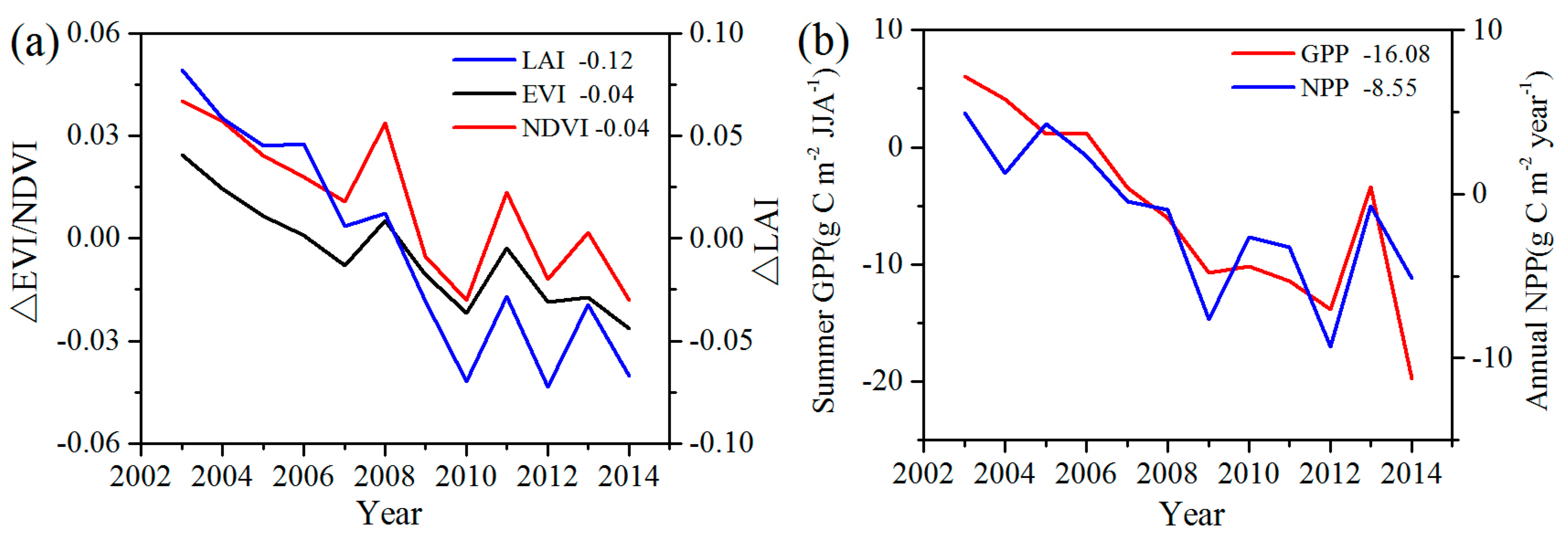
To analyze the quantitative effects of the WFs on vegetation growth and productivity for 2003–2014 in the study area, the area mean time series of differences in VI, GPP, and NPP between WFPs and NNWFPs (WFPs minus NNWFPs) are analyzed (Figure 5). Although the time series is short, the LAI, EVI, and NDVI differences all present significant downward trends, which are as follows: −0.15/11 years (p < 0.01), −0.04/11 years (p < 0.01) and −0.05/11 years (p < 0.01). The vegetation productivity also shows downward trends and the decreasing trends are −20.93 g C m−2/11 years (p < 0.01) for summer GPP and −10.19 g C m−2/11 years (p < 0.01) for annual NPP. Based on the vegetation index and productivity differences between post- and pre-turbines construction periods (2012–2014 minus 2003–2005), the effects of WFs on vegetation growth are quantified. From 2003 to 2014, the inhibiting effects of the WFs on vegetation growth are −0.12 (LAI), −0.04 (EVI), and −0.04 (NDVI), or 14.5%, 14.8%, and 8.9%, respectively, compared with the climatology values of 0.83 (LAI), 0.27 (EVI), and 0.45 (NDVI) for WFPs. The inhibiting effects of the WFs on vegetation productivity are −16.08 g C m−2 JJA−1 (GPP) and −8.55 g C m−2 year−1 (NPP), representing a change of 8.9% and 4.0% of the climatology value 180.81 g C m−2 JJA−1 and 214.86 g C m−2 year−1 over the WFPs. Note that the VI differences and vegetation productivity differences both remain relatively stable after 2012. The main reason for this trend may be that the wind turbine construction was essentially complete after 2012 and, as a result, the differences in VI, GPP and NPP between WFPs and NNWFPs gradually become stabilized. However, during the first few years, the number of wind turbines in WFPs gradually increased and, therefore, the differences between WFPs and NNWFPs gradually become larger (Figure 1a).
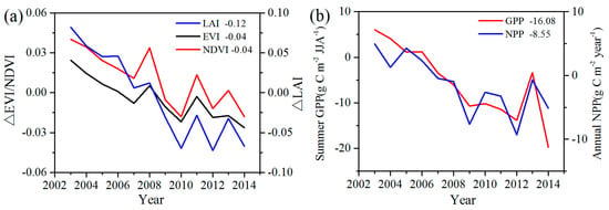
Figure 5.
Inter-annual variations of area mean (a) vegetation index differences and (b) GPP and NPP between WFPs and NNWFPs (WFPs minus NNWFPs) for the period 2003–2014. The insert numbers are the area mean VI, GPP, and NPP differences between the post- and pre-turbine construction periods (2012–2014 minus 2003–2005). WFPs and NNWFPs are defined as in Figure 2.
4. Discussion
In this paper, MODIS vegetation index and productivity data are used to analyze the effects of WFs on vegetation growth in the Bashang area in Northern China. The results show that the WFs have a significant inhibiting effect on vegetation growth and productivity both spatially and temporally. The potential processes, such as land-use change, differences in vegetation type, changes in climate, and wind speed and direction, may contribute to the inhibiting effect of vegetation growth.
Construction of WFs and other human activities change the land cover type, thus affecting the vegetation growth in the study area. In this research, Finer Resolution Observation and Monitoring of Global Land Cover (FROM-GLC) data for two periods in 2000 and 2010 are used to analyze land use changes in WFPs and NNWFPs in the study area. The spatial resolution of the data is 30 m [30]. The results show that the proportion of non-vegetation pixels (water and urban areas) in WFPs changes from 0.72% to 1.25%, while from 2000 to 2010, that in the NNWFPs changes from 2.50% to 3.48% (Figure S1). The proportions of the non-vegetation pixels and their changes in WFPs and NNWFPs are very small. Although the construction of wind turbines may indeed damage the vegetation canopy, the annual plants (grassland and crop) in the study area are able to recover quickly after being damaged in the next year (Figure S4). With the increase of the effect of WFs on daytime LST, vegetation growth cannot be restored to the level before the construction, or even continue to decrease, indicating that WFs do affect vegetation growth by changing the vegetation growth environment (Figure S4).
The difference in land cover types, such as different crop species and crop management, may also have potential influences on vegetation growth. For two main vegetation types in the WFPs and NNWFPs (crop and grass), the effects of the WFs are approximately the same (Figure S5). It is reasonable to assume that WFs have a similar effect on different crop species. The effect of crop species differences and crop managements would be much smaller than the strong and persistent signal of wind farm impacts. According to field campaigns, the support column of a wind turbine accounts for 4 m2, and 1747 wind turbines account for approximately 7000 m2, which represent a very small proportion (less than 0.1%) of the WFPs. Therefore, for the study area, land cover changes and differences in vegetation type for WFPs and NNWFPs have no significant effect on the underlying vegetation growth.
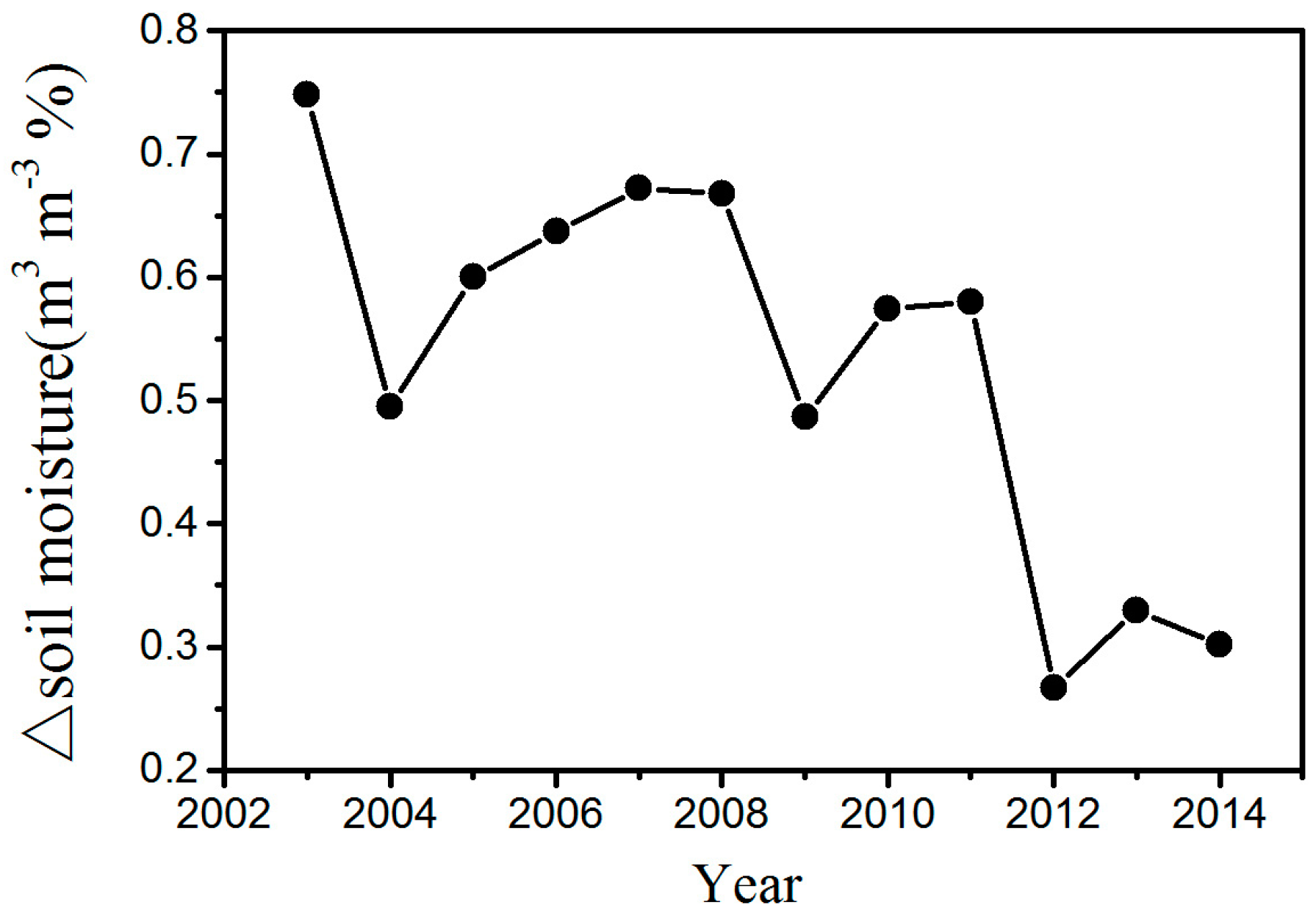
The changes in temperature may play an important role in the effect of WFs on vegetation growth. There is a warming effect of 0.15–0.18 °C coupled with WFs at night, which agrees with most existing studies (Figure 6b) [12,13,15]. The possible reason for this phenomenon is that the diurnal and seasonal variations in wind speed and the changes in near-surface atmospheric boundary layer (ABL) conditions due to wind turbines operations [9]. Contrary to some existing studies, this research finds that there is also a warming effect of 0.45–0.65 °C coupled with WFs during the daytime (Figure 6a). Zhou et al. [9] speculated that the possible reason is the slow development of the daytime unstable and convective layer [31]. Changes in ET may also play a role in daytime warming [32]. The ET in the WFPs is lower than that in the NNWFPs, and reduced transpiration may contribute to a higher LST in WFPs (Figure S6). In the study area, the LAI is negatively related to the daytime LST, and the correlations are all significant at a confidence level of 95% (Figure S7). The main reason for this trend may be that the WFs can reduce soil moisture through increasing LST in the study area (Figure 7). In this research, the study area is located in the semi-arid area of Northern China where soil moisture has a decisive effect on vegetation growth [16]. An increase in the LST reduces soil moisture and enhances water stress on vegetation growth. As a result, growth conditions for vegetation growth are suppressed, leading to a lower vegetation index. Furthermore, we also observed decreasing vegetation productivity in the WFs, which may be caused by inhibited photosynthesis through increasing water stress and enhanced autotrophic respiration through increasing nighttime temperatures.

Figure 6.
Summer MODIS LST anomaly differences (°C) between post- and pre-turbine-construction years (2012–2014 minus 2003–2005 averages) at (a) ~13:30 LT daytime and (b) ~01:30 LT nighttime. Plus symbols represent pixels with one or more wind turbines.
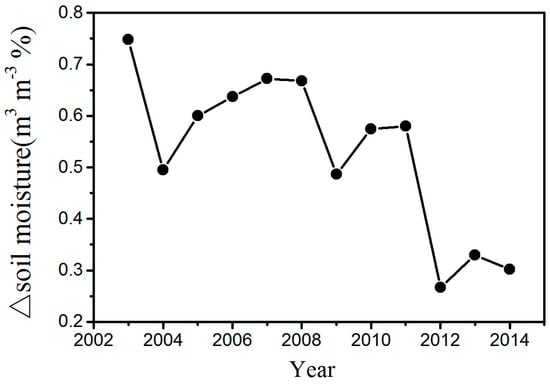
Figure 7.
Interannual variations of area mean soil moisture difference between WFPs and NNWFPs (WFPs minus NNWFPs) in the summer for the period 2003–2014.
Wind speed is the main factor determining energy conversion in wind turbines. Wind turbines have a cut-in and a cut-out wind speed, which are approximately 3–4 m/s and 20 m/s, respectively [10]. The wind speed in the study area is generally 4–8 m/s, meaning that the wind turbines can operate most of the time (Figure 8). Wind direction in the study area can affect the effects of WFs on LST, and thereby affect vegetation growth and productivity. Generally, the winds blow mainly from the southeast and northwest at night and from the southwest during the daytime (Figure 8). The positive LST anomaly differences all occur to the northwest and southeast of the WFs at night and to the northeast in the daytime (Figure 6). This result indicates that a downwind warming effect is occurring in the study area. To assess the downwind effect on vegetation growth, the SCI values of 5%, 10%, and 15% pixels of the smallest vegetation index anomaly differences located in UWFPs, DWFPs, and NNWFPs are compared with the corresponding SCI thresholds (5.3%, 6.3%, and 14.9%). The higher the SCI value of the DWFPs, the stronger the downwind effect. The SCI of the DWFPs ranges from 6.1% to 10.8% and 14 of the 15 are higher than the corresponding SCI thresholds (6.3%), indicating the existence of a downwind effect on vegetation growth (Table 1). In contrast, only 6 of the 15 SCI values for NNWFPs and none of the SCI values for UWFPs are higher than the corresponding SCI thresholds, indicating that the smallest vegetation index anomaly differences are unlikely to be found in the NNWFPs and UWFPs.
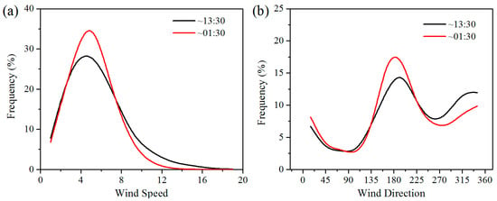
Figure 8.
Histogram of MERRA hourly 50 m (a) wind speed (m/s) and (b) direction in summer averaged over the study area during the period 2003–2014. Wind direction is determined by U- and V-components and measured in terms of degrees clockwise between 0 and 360(°). The wind from the North corresponds to 360° (0°), from the East corresponds to 90°, from the South corresponds to 180°, and from the West corresponds to 270°.
The main source of uncertainty in this paper comes from the errors in the MODIS vegetation index and productivity products [20,21,24]. Although the MODIS products represent the highest-quality retrieval data from clear-sky conditions, it still contains errors and noise due to clouds, aerosols, and the imperfection of the retrieval algorithms. In addition, there may be discrepancies in determining the positions of the wind turbines. The matching of various kinds of data of different resolutions may also produce errors in the results. However, the spatial and temporal averaging used in this paper can effectively reduce errors and uncertainties. The remaining residuals may not produce a spatial coupling between the layout of WFs and the vegetation index anomaly differences, especially when many different kinds of vegetation indexes are used.
5. Conclusions
In this study, the effects of WFs on the underlying vegetation growth in the Bashang area of Northern China are analyzed. The results show that WFs inhibit local vegetation growth and productivity, decreasing LAI, EVI, and NDVI by approximately 14.5%, 14.8%, and 8.9% from 2003 to 2014. There is an inhibiting effect of 8.9% on summer GPP and 4.0% on annual NPP over WFs. Potential reasons for the inhibiting effects are as follows: (1) inhibited photosynthesis through increasing water stress and enhanced autotrophic respiration through increasing daytime and nighttime temperatures and (2) downwind inhibited growth status and photosynthesis induced by the downwind warming effect. Our analysis provides clear observational evidence of the inhibiting effect on vegetation growth caused by WFs in the Bashang area of Northern China.
As the analysis is from a short period over a local region with rapid growth of wind farms, it should be kept in mind that the estimated inhibiting effects cannot be generally applied to other WFs. Wind farms affect the vegetation growth by changing local climate and damaging vegetation structures through constructions. For a given wind farm, the inhibiting effect should be quantified by fully considering local background environmental factors (e.g., temperature and soil moisture) and the recovery of vegetation with different vegetation conditions. Our results raise intriguing questions whether these suppressing patterns are observed in other WFs as well, and about trade-offs between production of clean energy and potential suppression of ecosystem functions.
Supplementary Materials
The following are available online at www.mdpi.com/2072-4292/9/4/332/s1. Figure S1: FROM-GLC land cover map in 2000 and their changes in 2010 at spatial resolutions of ~30 m; Figure S2. MODIS summer EVI climatology (2003–2011 averages); Figure S3: Summer MODIS EVI and NDVI differences between post- and pre-turbine-construction years; Figure S4: Inter-annual variations of area mean daytime LST and LAI differences in July, August and September; Figure S5: Inter-annual variations of area mean LAI and GPP differences of crop and grass between WFPs and NNWFPs; Figure S6: Summer MODIS ET and Albedo (%) differences between post- and pre-turbine-construction years; Figure S7: The spatial distribution map of the coefficient between summer MODIS LAI anomalies and LST anomalies.
Acknowledgments
The authors thank Jia Chen, Rongyun Tang, and Yifeng Peng for help in field measurements. We also thank Peipei Xu for helpful comments that improved this manuscript. This work was supported by the National Key Research and Development Program of China (No. 2016YFB0501404) and National Natural Science Foundation of China (No. 41331173). Data associated with this research (location of wind turbines and other climate data) can be obtained from the corresponding author via e-mail (zhaoxiang@bnu.edu.cn).
Author Contributions
Bijian Tang and Donghai Wu conceived of and designed the experiments. Bijian Tang processed and analyzed the data. All authors contributed to the ideas, writing, and discussion.
Conflicts of Interest
The authors declare no conflict of interest.
References
- Rajewski, D.A.; Takle, E.S.; Lundquist, J.K.; Prueger, J.H.; Pfeiffer, R.L.; Hatfield, J.L.; Spoth, K.K.; Doorenbos, R.K. Changes in fluxes of heat, H2O, and CO2 caused by a large wind farm. Agric. For. Meteorol. 2014, 194, 175–187. [Google Scholar] [CrossRef]
- Armstrong, A.; Waldron, S.; Whitaker, J.; Ostle, N.J. Wind farm and solar park effects on plant-soil carbon cycling: Uncertain impacts of changes in ground-level microclimate. Glob. Chang. Biol. 2014, 20, 1699–1706. [Google Scholar] [CrossRef] [PubMed]
- Balog, I.; Ruti, P.M.; Tobin, I.; Armenio, V.; Vautard, R. A numerical approach for planning offshore wind farms from regional to local scales over the mediterranean. Renew. Energy 2016, 85, 395–405. [Google Scholar] [CrossRef]
- Vautard, R.; Thais, F.; Tobin, I.; Bréon, F.-M.; de Lavergne, J.-G.D.; Colette, A.; Yiou, P.; Ruti, P.M. Regional climate model simulations indicate limited climatic impacts by operational and planned european wind farms. Nat. Commun. 2014, 5. [Google Scholar] [CrossRef] [PubMed]
- Roy, S.B.; Traiteur, J.J. Impacts of wind farms on surface air temperatures. Proc. Natl. Acad. Sci. USA 2010, 107, 17899–17904. [Google Scholar]
- Fiedler, B.; Bukovsky, M. The effect of a giant wind farm on precipitation in a regional climate model. Environ. Res. Lett. 2011, 6, 045101. [Google Scholar] [CrossRef]
- Jacobson, M.Z.; Archer, C.L.; Kempton, W. Taming hurricanes with arrays of offshore wind turbines. Nat. Clim. Chang. 2014, 4, 195–200. [Google Scholar] [CrossRef]
- Fitch, A.C.; Lundquist, J.K.; Olson, J.B. Mesoscale influences of wind farms throughout a diurnal cycle. Mon. Weather Rev. 2013, 141, 2173–2198. [Google Scholar] [CrossRef]
- Zhou, L.; Tian, Y.; Roy, S.B.; Thorncroft, C.; Bosart, L.F.; Hu, Y. Impacts of wind farms on land surface temperature. Nat. Clim. Chang. 2012, 2, 539–543. [Google Scholar] [CrossRef]
- Zhou, L.; Tian, Y.; Roy, S.B.; Dai, Y.; Chen, H. Diurnal and seasonal variations of wind farm impacts on land surface temperature over western texas. Clim. Dyn. 2013, 41, 307–326. [Google Scholar] [CrossRef]
- Zhou, L.; Tian, Y.; Chen, H.; Dai, Y.; Harris, R.A. Effects of topography on assessing wind farm impacts using modis data. Earth Interact. 2013, 17, 1–18. [Google Scholar] [CrossRef]
- Xia, G.; Zhou, L.; Freedman, J.M.; Roy, S.B.; Harris, R.A.; Cervarich, M.C. A case study of effects of atmospheric boundary layer turbulence, wind speed, and stability on wind farm induced temperature changes using observations from a field campaign. Clim. Dyn. 2016, 46, 2179–2196. [Google Scholar] [CrossRef]
- Harris, R.A.; Zhou, L.; Xia, G. Satellite observations of wind farm impacts on nocturnal land surface temperature in iowa. Remote Sens. 2014, 6, 12234–12246. [Google Scholar] [CrossRef]
- Slawsky, L.; Zhou, L.; Roy, S.; Xia, G.; Vuille, M.; Harris, R. Observed thermal impacts of wind farms over northern illinois. Sensors 2015, 15, 14981. [Google Scholar] [CrossRef] [PubMed]
- Chang, R.; Zhu, R.; Guo, P. A case study of land-surface-temperature impact from large-scale deployment of wind farms in china from guazhou. Remote Sens. 2016, 8, 790. [Google Scholar] [CrossRef]
- Wu, D.; Zhao, X.; Liang, S.; Zhou, T.; Huang, K.; Tang, B.; Zhao, W. Time-lag effects of global vegetation responses to climate change. Glob. Chang. Biol. 2015, 21, 3520–3531. [Google Scholar] [CrossRef] [PubMed]
- Lin, Y.; Tu, L.; Liu, H.; Li, W. Fault analysis of wind turbines in china. Renew. Sustain. Energy Rev. 2016, 55, 482–490. [Google Scholar] [CrossRef]
- Leung, D.Y.; Yang, Y. Wind energy development and its environmental impact: A review. Renew. Sustain. Energy Rev. 2012, 16, 1031–1039. [Google Scholar] [CrossRef]
- Sun, S.; Liu, F.; Xue, S.; Zeng, M.; Zeng, F. Review on wind power development in china: Current situation and improvement strategies to realize future development. Renew. Sustain. Energy Rev. 2015, 45, 589–599. [Google Scholar] [CrossRef]
- Huete, A.; Didan, K.; Miura, T.; Rodriguez, E.P.; Gao, X.; Ferreira, L.G. Overview of the radiometric and biophysical performance of the modis vegetation indices. Remote Sens. Environ. 2002, 83, 195–213. [Google Scholar] [CrossRef]
- Zhao, M.; Heinsch, F.A.; Nemani, R.R.; Running, S.W. Improvements of the modis terrestrial gross and net primary production global data set. Remote Sens. Environ. 2005, 95, 164–176. [Google Scholar] [CrossRef]
- Running, S.W.; Nemani, R.R.; Heinsch, F.A.; Zhao, M.; Reeves, M.; Hashimoto, H. A continuous satellite-derived measure of global terrestrial primary production. Bioscience 2004, 54, 547–560. [Google Scholar] [CrossRef]
- Rienecker, M.M.; Suarez, M.J.; Gelaro, R.; Todling, R.; Bacmeister, J.; Liu, E.; Bosilovich, M.G.; Schubert, S.D.; Takacs, L.; Kim, G.-K. Merra: Nasa’s modern-era retrospective analysis for research and applications. J. Clim. 2011, 24, 3624–3648. [Google Scholar] [CrossRef]
- Schaaf, C.B.; Gao, F.; Strahler, A.H.; Lucht, W.; Li, X.; Tsang, T.; Strugnell, N.C.; Zhang, X.; Jin, Y.; Muller, J.-P. First operational brdf, albedo nadir reflectance products from modis. Remote Sens. Environ. 2002, 83, 135–148. [Google Scholar] [CrossRef]
- Mu, Q.; Zhao, M.; Running, S.W. Improvements to a modis global terrestrial evapotranspiration algorithm. Remote Sens. Environ. 2011, 115, 1781–1800. [Google Scholar] [CrossRef]
- Wan, Z. New refinements and validation of the modis land-surface temperature/emissivity products. Remote Sens. Environ. 2008, 112, 59–74. [Google Scholar] [CrossRef]
- Liu, Y.; Dorigo, W.A.; Parinussa, R.; de Jeu, R.A.; Wagner, W.; McCabe, M.F.; Evans, J.; Van Dijk, A. Trend-preserving blending of passive and active microwave soil moisture retrievals. Remote Sens. Environ. 2012, 123, 280–297. [Google Scholar] [CrossRef]
- Kumar, V.; Svensson, G.; Holtslag, A.; Meneveau, C.; Parlange, M.B. Impact of surface flux formulations and geostrophic forcing on large-eddy simulations of diurnal atmospheric boundary layer flow. J. Appl. Meteorol. Climatol. 2010, 49, 1496–1516. [Google Scholar] [CrossRef]
- Barthelmie, R.J.; Pryor, S.; Frandsen, S.T.; Hansen, K.S.; Schepers, J.; Rados, K.; Schlez, W.; Neubert, A.; Jensen, L.; Neckelmann, S. Quantifying the impact of wind turbine wakes on power output at offshore wind farms. J. Atmos. Ocean. Technol. 2010, 27, 1302–1317. [Google Scholar] [CrossRef]
- Gong, P.; Wang, J.; Yu, L.; Zhao, Y.; Zhao, Y.; Liang, L.; Niu, Z.; Huang, X.; Fu, H.; Liu, S. Finer resolution observation and monitoring of global land cover: First mapping results with landsat tm and etm+ data. Int. J. Remote Sens. 2013, 34, 2607–2654. [Google Scholar] [CrossRef]
- Stull, R.B. An Introduction to Boundary Layer Meteorology; Springer Science & Business Media: Berlin, Germany, 2012; Volume 13. [Google Scholar]
- Baidya Roy, S.; Pacala, S.W.; Walko, R.L. Can large wind farms affect local meteorology? J. Geophys. Res. Atmos. 2004, 109. [Google Scholar] [CrossRef]
© 2017 by the authors. Licensee MDPI, Basel, Switzerland. This article is an open access article distributed under the terms and conditions of the Creative Commons Attribution (CC BY) license (http://creativecommons.org/licenses/by/4.0/).

