First Results from Sentinel-1A InSAR over Australia: Application to the Perth Basin

Abstract

Past ground-based geodetic measurements in the Perth Basin, Australia, record small-magnitude subsidence (up to 7 mm/y), but are limited to discrete points or traverses across parts of the metropolitan area. Here, we investigate deformation over a much larger region by performing the first application of Sentinel-1A InSAR data to Australia. The duration of the study is short (0.7 y), as dictated by the availability of Sentinel-1A data. Despite this limited observation period, verification of Sentinel-1A with continuous GPS and independent TerraSAR-X provides new insights into the deformation field of the Perth Basin. The displacements recorded by each satellite are in agreement, identifying broad (>5 km wide) areas of subsidence at rates up to 15 mm/y. Subsidence at rates greater than 20 mm/y over smaller regions (∼2 km wide) is coincident with wetland areas, where displacements are temporally correlated with changes in groundwater levels in the unconfined aquifer. Longer InSAR time series are required to determine whether these measured displacements are representative of long-term deformation or (more likely) seasonal variations. However, the agreement between datasets demonstrates the ability of Sentinel-1A to detect small-magnitude deformation over different spatial scales (from 2 km–10 s of km) in the Perth Basin. We suggest that, even over short time periods, these data are useful as a reconnaissance tool to identify regions for subsequent targeted studies, particularly given the large swath size of radar acquisitions, which facilitates analysis of a broader portion of the deformation field than ground-based methods or single scenes of TerraSAR-X.

1. Introduction

Small-magnitude subsidence (up to 7 mm/y) has been measured in Perth, Australia (Figure 1) and is attributed to groundwater extraction [1]. Such ground deformation is common and well documented in other expanding population centres, where increased demand is placed on aquifers to meet domestic, industrial and agricultural water needs (Galloway and Burbey [2] and the references therein). Land subsidence may cause: increased risk of seawater inundation [3,4]; damage to infrastructure [5]; and compromised integrity of geodetic benchmarks [6]. Ongoing geodetic measurements are therefore required to monitor subsidence and may also provide constraints on spatio-temporal aquifer dynamics [7], which is of significance to groundwater-resource management.

In the Perth Basin, the small magnitude of deformation and limited historical geodetic infrastructure mean that measuring subsidence has previously been problematic [8]. Past measurements of subsidence are derived from repeat levelling between Fremantle and Hillarys (Figure 2), plus two public-domain continuous GPS receivers located at Hillarys (HIL1 in Figure 2) and ∼14 km east of Hillarys towards the Swan Valley (PERT in Figure 2) [1]. Whilst repeat levelling offers high precision [9], repeat surveys are labour intensive and are therefore only carried out over a limited area or after large time intervals. Continuous GPS provides measurements at high temporal resolution (∼30 s), but only at discrete spatial locations. These geodetic methods therefore do not capture the full complexity of the deformation field in space and/or time, and additional time series of measurements are required over larger areas and at higher spatial and temporal resolutions.

One such tool to achieve this is interferometric synthetic aperture radar (InSAR). Since the early 1990s, InSAR has become an increasingly popular method for measuring ground deformation over a range of spatial scales, from individual buildings or structures [10] to continents [11]. InSAR operates by comparing the phase of time-separated satellite radar images acquired over the same region (for further details, we refer the reader to Bürgmann et al. [12], Hanssen [13], Massonnet and Feigl [14], Simons and Rosen [15]). Preliminary InSAR studies of the Perth Basin between 1992 and 1997 reported subsidence rates of up to 50 mm/y [16]; however, this was later disproved by Dawson [17], who found that average subsidence rates did not exceed ∼4 mm/y over this time.

In April 2014, the European Space Agency (ESA) launched Sentinel-1A, the first half of a two-satellite constellation providing the most extensive and systematic coverage of SAR data to date [18] and the first mission to deliver data on a near-real-time, open-access basis. Sentinel-1A data have since been used to make observations of deformation that is centimetres-to-metres in magnitude, associated with earthquakes (e.g., Mw 7.8 Gorkha, Nepal: [19,20,21,22]); volcanic eruptions (e.g., Fogo, Cape Verde: [23]); and the development of sink holes (e.g., Wink, Texas: [24]). However, the detection of small-magnitude displacements, such as subsidence of the Perth Basin, is reliant on longer time series of images.

Mainland Australia was fully imaged during the initial phase of Sentinel-1A. However, only a limited spatial coverage of repeat images has subsequently been acquired. Repeated coverage is densest over Victoria and New South Wales, where to date, over 60 scenes have been acquired 10 times or more (Figure 1). In Western Australia, this level of repeat has only been achieved in two locations, including over the Perth Basin (Figure 1).

In this study, we first review the previous use of InSAR over Australia, commenting on the availability of data and the relatively small number of peer-reviewed studies. We then describe an application of Sentinel-1A data to the Perth Basin, validating the observations with an independent TerraSAR-X InSAR survey over the same time period. In doing so, we carry out a reconnaissance investigation into the larger extent of the deformation field in the Perth Basin, whilst demonstrating the applicability of Sentinel-1A to measure small-magnitude deformation associated with changes in groundwater levels. Using these observations, we highlight the importance of ongoing time series of InSAR data to measure subsidence due to groundwater extraction throughout this population centre.

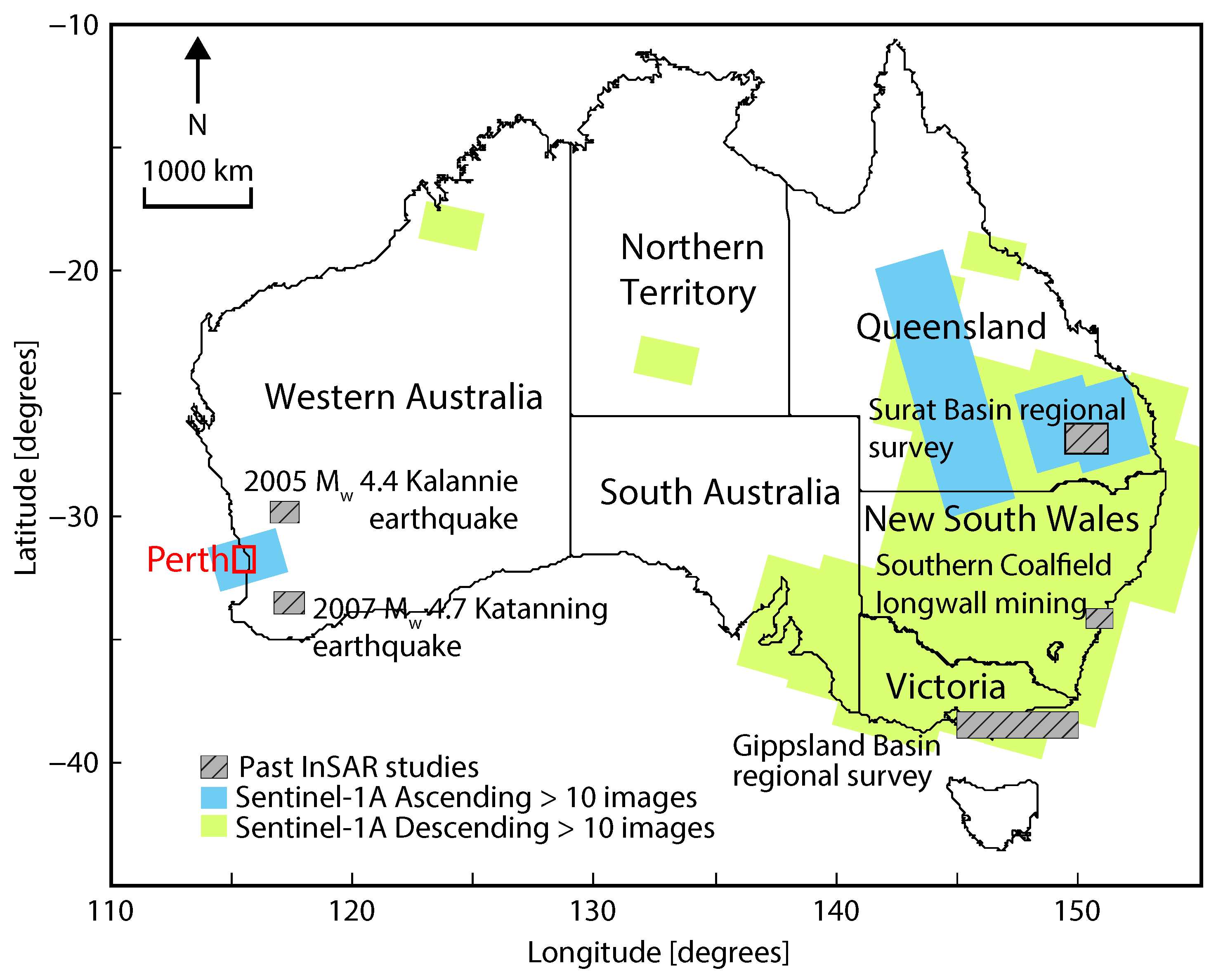
2. Previous Use of InSAR over Australia

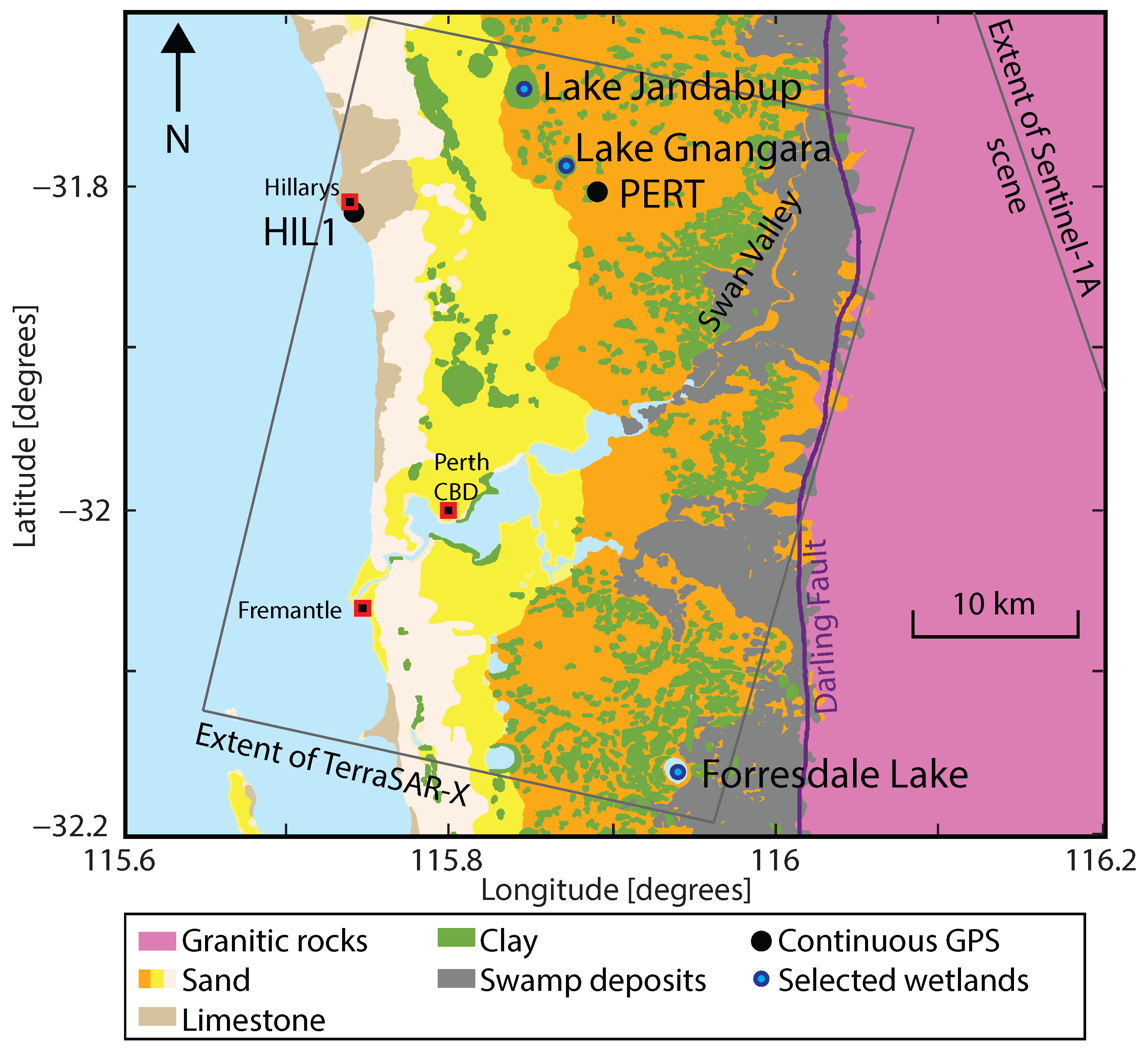
The spatial and temporal coverage of InSAR data over mainland Australia has been variable, and overall, the density of satellite acquisitions has been less than that over other continents. Situated in a relatively stable intraplate setting, mainland Australia has an absence of active volcanoes (as recognised by the Smithsonian Global Volcanism Program: http://volcano.si.edu) and low-to-moderate seismicity compared to the world average [25], both of which have been used to inform past and present satellite acquisition strategies [26]. However, large-magnitude (M${}_w$ > 6) earthquakes do occur [27], and intraplate seismicity tends to be unusually shallow [28], therefore being more likely to cause ground displacements and/or surface rupture [29]. Coseismic deformation has been observed with InSAR in the South West Seismic Zone (Figure 1), including the $M_w$ 4.4 2005 Kalannie earthquake sequence, one of the smallest magnitude earthquakes linked to ground deformation detected using InSAR [30], and the 2007 Katanning $M_w$ 4.7 earthquake, which caused up to 320 mm of displacement in the satellite line of sight [30,31].

Other peer-reviewed InSAR studies of Australia document ground deformation induced by anthropogenic activities, predominantly underground longwall coal mining in New South Wales, which is linked to horizontal and vertical displacements of 10 s of mm/y and 100 s of mm/y, respectively [32,33,34,35,36] (Figure 1). Elsewhere, regional-scale InSAR surveys have been implemented, including in the Gippsland Basin, Victoria. Here, ALOS data spanning 14,000 km${}^2$ were used to measure subsidence arising from open-cut mining and groundwater extraction and subsequently to assess the susceptibility of nearby coastal regions to sea-level rise [37]. Similarly, in the Surat Basin, Queensland (Figure 1), regional-scale InSAR reveals more than 20 mm/y of subsidence due to the extraction of coal bed methane and associated groundwater [38]. Monitoring of the Surat Basin includes a network of 40 corner reflectors installed by Geoscience Australia to tie relative ground displacements recorded by InSAR to GNSS [39] and also act as a calibration site for Sentinel-1 [26].

The diversity of the above studies reflects the wide range of applications of InSAR data in Australia, but the small number of peer-reviewed studies shows that the uptake of this technique has been relatively slow. This is likely related to the sparsity of data, particularly in the north and west of the continent (e.g., Figure 1), although this is subject to change with the launch of new satellite missions. At the time of writing, the second half of the Sentinel constellation, Sentinel-1B, has begun to acquire data Australia-wide at 12-day repeat intervals. Such increases in data coverage will aid in enabling wider application of InSAR to measure ground deformation driven by anthropogenic and geological/hydrogeological factors.

3. Study Area

The city of Perth is located on the Swan Coastal Plain in the central portion of the Perth Basin, an elongated Cainozioc/Mesozoic sedimentary formation spanning ∼1000 km northwards from the southwestern tip of Australia [40]. The eastern margin is adjacent to the Archean Yilgarn Craton (granitic rocks in Figure 2) and is bounded by the near-vertical Darling Fault [41,42]. The Darling Scarp is located 1 km–3 km east of the Darling Fault and rises steeply ∼200 m above the Basin, dominating the topography of the region. To the west, the Perth Basin extends for ∼150 km beneath the Indian Ocean towards the continental rise [40].

The sedimentary succession in the Perth region is ∼12 km thick [40] and houses numerous freshwater aquifers, the shallowest of which is the unconfined (superficial) aquifer extending to depths up to 70 m [43]. The surface geology that constitutes the unconfined aquifer ranges from clay close to the Darling Scarp, through a succession of fixed sand dunes in the central coastal plain, to limestone along the coastal belt [43] (Figure 2). In northern Perth, the unconfined aquifer is underlain by the semi-confined Mirrabooka aquifer with a thickness up to 160 m [43]. Spanning the entire Perth region are two major confined aquifers that consist of laterally discontinuous siltstones, sandstones and shales. The shallower Leederville aquifer has a thickness of 50 m to more than 550 m, and the deeper Yarragadee aquifer has a thickness of more than 2 km [43]. These four aquifers are the most significant and extensively exploited groundwater resources in the Perth Basin.

Groundwater provides ∼45% of the total water requirement in the Perth Region, with a comparable amount derived from the desalination of seawater. Extraction from the Leederville aquifer began in 1974 and has continued at a rate of ∼1.41 GL/y. Extraction from the Yarragadee commenced in 1979 and increased dramatically between the early 1990s and 2005 from 0.25 GL/y–3.72 GL/y, with the addition of new production bores in northern Perth. Since 2005, the rate of extraction from the Yarragadee has decreased by ∼1 GL/y [1]. In addition to managed extraction from the confined aquifers, significant extraction occurs from the unconfined aquifer, including from more than 70,000 shallow, private bores (personal communication: Western Australian Department of Water).

Changes in the rates of groundwater extraction and recharge are reflected in measurements of hydraulic head (i.e., the elevation to which water rises in a well) made by the Western Australian Department of Water at artesian monitoring bores. Measurements are made on either a quasi-monthly basis or as daily averages derived from continuous loggers and are accessible via the Department of Water Information Reporting Service (http://wir.water.wa.gov.au/Pages/Water-Information-Reporting.aspx).

4. InSAR Datasets and Methods

We investigate ground displacements in the Perth Basin using temporally- and spatially- overlapping Sentinel-1A (C-band: $\lambda$ ∼ 56 mm) and TerraSAR-X (X-band: $\lambda$ ∼ 31 mm) datasets. All interferograms were produced using the JPL/Caltech InSAR Scientific Computing Environment (ISCE) software [44], with different processing chains implemented for each dataset to account for differences in the satellite acquisition modes. Multi-temporal analysis was then used to combine the interferograms in each dataset and increase the signal-to-noise ratio [45].

4.1. Sentinel-1A and TerraSAR-X Datasets

Over Perth, Sentinel-1A acquisitions were made in an ascending orbit at 24-day intervals (i.e., every other cycle) between 27 August 2015 and 17 May 2016 (12 images in total). Four descending scenes are also available between November 2015 and March 2016, but due to the long and irregular acquisition intervals between these images, we do not include these data in this study.

Sentinel-1A data are provided via the online Sentinel-1 Scientific Data Hub in Interferometric Wide-swath (IW) focused Single Look Complex (SLC) format. Each SLC is split into three sub-swaths that are subsequently subdivided into ∼10 bursts. In total, the IW SLCs are ∼150 km in the along-track direction and ∼250 km across-track, with a spatial resolution (pixel size) of ∼14 m. We use the central sub swath, which covers the Perth metropolitan area and is ∼85 km across-track (Figure 2).

We use 22 TerraSAR-X images obtained from the German Aerospace Center (DLR) under science project LAN1499, that cover the same time period as the Sentinel-1A dataset to within four days (29 August 2015–19 May 2016). Images are separated by 11-day intervals, with the exception of a 33-day gap in March 2016. Unlike the Sentinel-1A dataset, all imagery was acquired in a descending orbit in strip map mode. The images have a higher spatial resolution than Sentinel-1A (∼3 m pixels), but cover a smaller area that is ∼50 km and ∼35 km in the along- and across-track directions, respectively (Figure 2).

4.2. Interferogram Formation

TerraSAR-X interferograms were produced using processing workflows that are well documented in the literature (e.g., [12]) and are implemented in the ISCE software. For Sentinel-1A imagery collected using the TOPS (Terrain Observation with Progressive Scans) [18] acquisition strategy, there are several variations to the interferogram processing sequence that must be taken to deburst and merge the swath whilst avoiding phase offsets.

Firstly, Sentinel-1A IW SLCs that are processed with different versions of the instrument performance facility use different elevation antenna patterns, resulting in range-varying phase offsets that require correction at either the SLC or interferogram level [46]. Within ISCE, coregistration of the master and slave SLCs is then performed on a burst-by-burst, rather than full image basis, with the assistance of a digital surface model (we use a 30-m digital surface model derived from the Shuttle Radar Topography Mission: [47]) and precise orbits [48] that are released by ESA ∼20 days after each acquisition. Coarse offsets and interferograms are calculated for the regions of burst overlap only.

As TOPS generates a high Doppler rate in azimuth, a very precise coregistration to one thousandth of a pixel in azimuth is required to avoid phase ramps across individual bursts and phase discontinuities between bursts [49,50]. This is achieved by performing enhanced spectral diversity on the burst overlap interferograms [49] and is followed by estimation of the range misregistration using the amplitude correlation of the overlap regions. Next, fine offsets are estimated for each complete burst, and burst-by-burst interferograms are produced. The burst interferograms are then merged to produce a continuous sub-swath resulting in a strip map-like product.

Interferograms for both datasets were filtered [51], unwrapped using the statistical-cost network-flow algorithm for phase unwrapping (SNAPHU) [52], geocoded and multi-looked (spatially averaged) to a final spatial resolution of ∼90 m (e.g., [53]). To facilitate comparisons between the two datasets, the unwrapped interferogram phase was lastly converted to vertical displacement using the look angle of each satellite [54]. This conversion is justified because the satellite line of sight is most sensitive to vertical displacements [55], and there is no evidence for differential horizontal ground motion across the Perth Basin between continuous GPS receivers HIL1 and PERT. Throughout this study, positive displacements therefore indicate ground movement towards the satellite (relative uplift), and negative displacements indicate movement away from the satellite (relative subsidence).

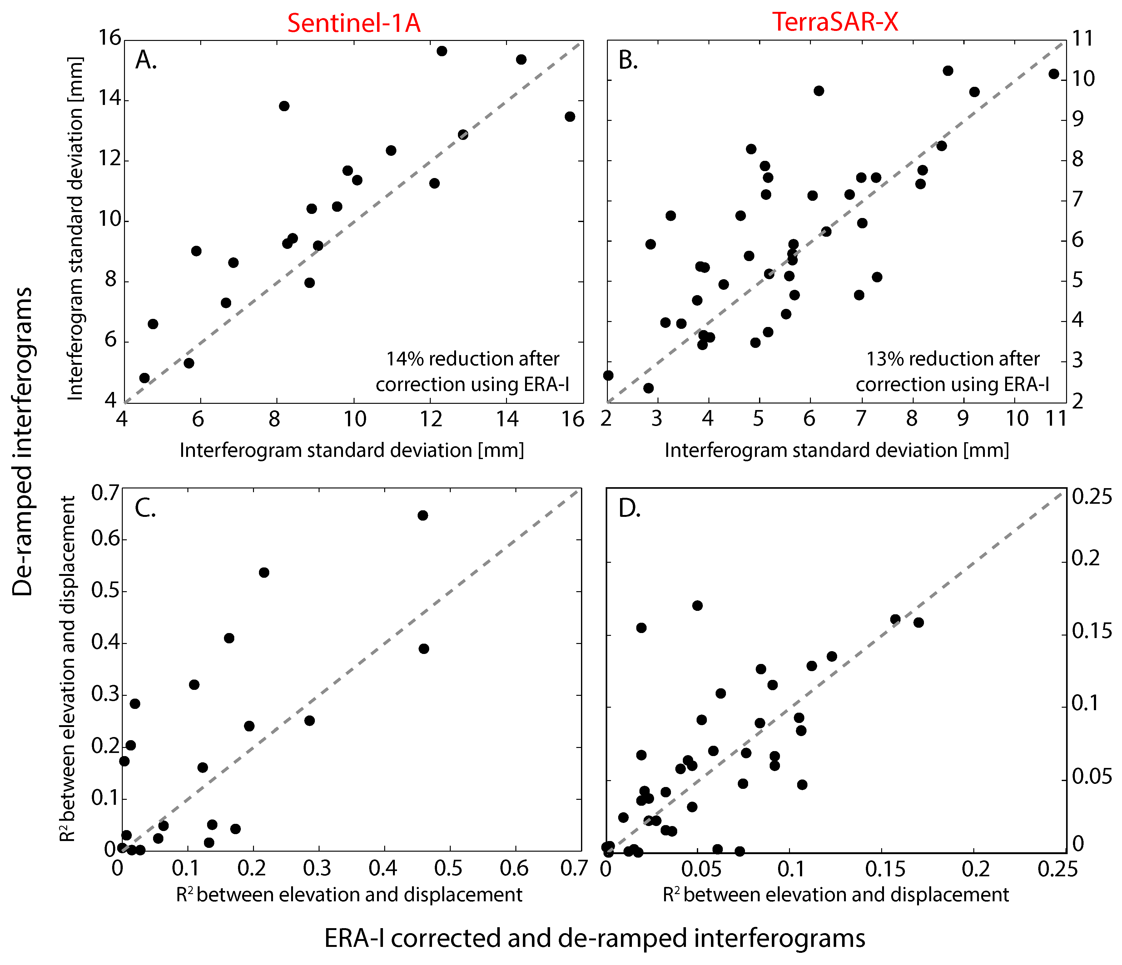
4.3. Reduction of Error Sources

Following unwrapping, the interferograms contain residual unwrapping errors that appear as 2$\pi$ phase jumps, particularly in regions of low coherence. These errors are identified under the knowledge that the phase field is conservative, i.e., for acquisitions at Epochs 1, 2 and 3, the phase of interferogram ${\varphi }_{1,3}$ is equal to the sum of the phase of interferograms ${\varphi }_{1,2}$ and ${\varphi }_{2,3}$ [56]. Consecutive loops of interferograms were therefore used to isolate and mask any phase unwrapping errors.

The resulting interferogram phase contains contributions from various noise sources, most notably changes in atmospheric conditions (pressure, temperature, water vapour content) between acquisitions, causing artefacts that are typically a few cm in magnitude [13,57]. The atmospheric contribution to phase is commonly divided into stratified and turbulent components [13]. The long-wavelength (>10 km), stratified component includes phase signals that correlate with topography due to vertical stratification of the atmosphere [58]. In the Perth Basin, these artefacts are most likely to occur across the ∼200-m elevation of the Darling Scarp in the east of the TerraSAR-X and Sentinel-1A scenes. The short-wavelength (<10 km) turbulent component is attributed to lateral changes in the distribution of water vapour over short time intervals, which results in spatially- and temporally-random phase patterns. Whilst these turbulent features may be reduced by temporal averaging [59], the stratified component is likely to have a seasonal dependence that can bias deformation estimates [58] and should therefore be estimated and removed.

There are various approaches for correcting atmospheric artefacts in interferograms (for examples, see Parker et al. [60] and the references therein), including empirical methods that utilise statistical properties of the data, most commonly the relationship between interferogram phase and elevation, to estimate the stratified contribution [61]. The success of this approach typically relies upon prior knowledge of either the location or spatial wavelength of deformation [62], of which we have neither in the Perth Basin. Predictive methods use external datasets, such as large-scale weather models [58,63] or GPS [64,65], to calculate and remove atmospheric artefacts. There are only two public-domain continuously operating GPS receivers in the Perth Basin (Figure 2), which is insufficient to use the latter approach. Instead, we estimate the stratified component of the atmospheric error using the ERA-Interim (ERA-I) global atmospheric reanalysis. This is a freely available tool from the European Centre for Medium-Range Weather Forecasts and has been used successfully to correct interferograms in a variety of atmospheric settings [58,60,66,67]. ERA-I provides estimates of temperature, geopotential height and relative humidity at 37 pressure levels between 100 hPa and 1 hPa, on a 75 km × 75 km global grid, at six-hourly intervals [68,69,70]. We select the model cycle closest to the SAR acquisition time for each satellite (within 1 h) and combine the model outputs with a digital surface model using the method described in Jolivet et al. [66] and Walters et al. [67] to produce 2D maps of atmospheric delay. Differential maps of atmospheric delay are then subtracted from the interferograms.

The final step of error correction is to empirically estimate and remove the best-fitting planar phase ramp representing the orbital error contribution to phase and any residual long wavelength atmospheric signals [13,56,71].

4.4. Stacking and Time Series Analysis

Ground displacements from InSAR are measured relative to a region that is either assumed to be stable (zero displacement) or is deforming in a way that is well characterised by other data. We take the former approach and identify a suitable reference region by calculating the standard deviation of each pixel in both datasets, selecting a point that has a low standard deviation and is therefore unlikely to be undergoing large displacements. However, surface motion in this region cannot be completely ruled out, and any displacements will propagate through the entire scene. An alternative approach would be to select a reference region on the stable Yilgarn Craton, but the extent of the TerraSAR-X swath restricts this to an area proximal to the Darling Scarp (Figure 2), where there may be residual artefacts due to atmospheric stratification.

After all interferograms are adjusted to the reference region, we perform stacking and time series analysis. Firstly, interferogram displacements at each pixel are summed together and divided by the total duration of the observations to create deformation rate-maps for each dataset that are scaled to give annual rates of vertical displacement. Profiles are then extracted across areas of interest from west to east along lines of latitude by selecting a band that is 10 pixels (∼1 km) wide. The errors on the profiles represent 2 $\sigma$ of these values.

Up to 90% of the annual rainfall in Perth occurs between April and October [72]. Ground displacements occurring due to near-surface hydrological changes are therefore likely to exhibit a seasonal dependence, which is observed in previous time series at the two publicly-operating continuous GPS receivers PERT and HIL1 [1] (Figure 2). To produce time series from the sets of interferograms, we solve for the cumulative displacement at each epoch using a least squares approach [73,74]. Errors on the displacement measurements are estimated using Monte Carlo analysis [75]. Randomly-generated atmospheric noise was added to the data prior to the inversion, and the error bars represent 2 $\sigma$ of the resulting displacement values.

We validate the measurements from InSAR with ground-truth data by comparing InSAR time series calculated at the five pixels closest to each GPS (HIL1 and PERT) to time series of the vertical GPS displacement components obtained from the Nevada Geodetic Laboratory (http://geodesy.unr.edu/NGLStationPages/gpsnetmap/GPSNetMap.html). Unlike the GPS, InSAR measurements are not in a geocentric reference frame, and so, to compare the two types of data, we compute time series of displacements at HIL1 relative to PERT.

5. Results

5.1. Interferograms

In total, we produced 11 consecutive Sentinel-1A interferograms and 21 consecutive TerraSAR-X interferograms. We evaluate the performance of the stratified atmospheric correction by comparing the interferogram standard deviation before and after application of ERA-I [60,76]. Before comparison, non-ERA-I-corrected interferograms were de-ramped using the method described in Section 4.3. The reduction in interferogram standard deviation between the two datasets is comparable, with a 14% reduction for Sentinel-1A and 13% reduction for TerraSAR-X (Figure 3A,B).

In a second test, we compared the correlation between pixel displacement and pixel elevation before and after correction using the coefficient of determination $R^2$ metric [60,63]. Larger values of $R^2$ are observed for the non-corrected datasets (Figure 3C,D), suggesting that application of ERA-I has reduced the effects of stratified atmospheric noise and the correlation between displacements and topography. However, we do not expect this method to correct all atmospheric signals, and in both datasets, we observe other phase patterns including quasi-systematic banding, which has been attributed to gravity waves in the atmosphere and observed in other coastal locations [76].

Due to its longer sensor wavelength, Sentinel-1A interferograms are ∼20% more coherent than TerraSAR-X interferograms, but overall, both datasets are coherent over much of the study area (Figure 4A,B). Incoherence in both datasets is greatest in agricultural/bushland regions northeast of the Perth central business district close to the Swan Valley and southeast of Fremantle (Figure 2). Incoherence in the Sentinel-1A dataset also occurs over forests east of the Darling Scarp.

5.2. Multi-Temporal Analysis

Despite the short time period of observation (0.7 y), deformation rate-maps produced for the overlapping Sentinel-1A and TerraSAR-X datasets show comparable results (Figure 4A–C), and time series of the vertical displacements recorded by both satellites are within the error of those measured using GPS (Figure 4D), placing further confidence in the InSAR measurements over the short observation period.

From the deformation rate-maps, we identify features of the deformation field that are evident in both InSAR datasets, verifying the application of Sentinel-1A with independent evidence from TerraSAR-X and also providing more information about a greater spatial extent of the deformation field in the Perth Basin than has previously been given by repeat levelling or continuous GPS [1]. We classify the observed displacements into three categories according to the magnitude and spatial extent of the deformation [54,77]. These are: (1) broad regions (>5 km wide) of low magnitude (up to 15 mm/y) relative subsidence (labelled (a) in Figure 4); (2) elongated regions of adjacent relative uplift and subsidence (rectangle labelled (b) in Figure 4); and (3) localised (∼2 km wide) relative subsidence at rates of greater than 20 mm/y coincident with wetland areas (labelled (c1, c2, c3) in Figure 4).

In addition to these displacements, we observe other phase patterns that do not correlate between datasets, suggesting they are likely due to remaining atmospheric noise (Figure 4A,B). This may arise due to differences between the time of the Sentinel-1A and TerraSAR-X acquisitions and the time of ERA-I model simulation or atmospheric turbulence that is not captured by the model parameters [60]. Most notably, in the northeastern part of the TerraSAR-X stack (Figure 4B), there is a positive signal, which we attribute to unmodelled residual atmospheric stratification across the Darling Scarp (to compare the atmospherically-corrected and uncorrected deformation rate-maps, see Figure S1).

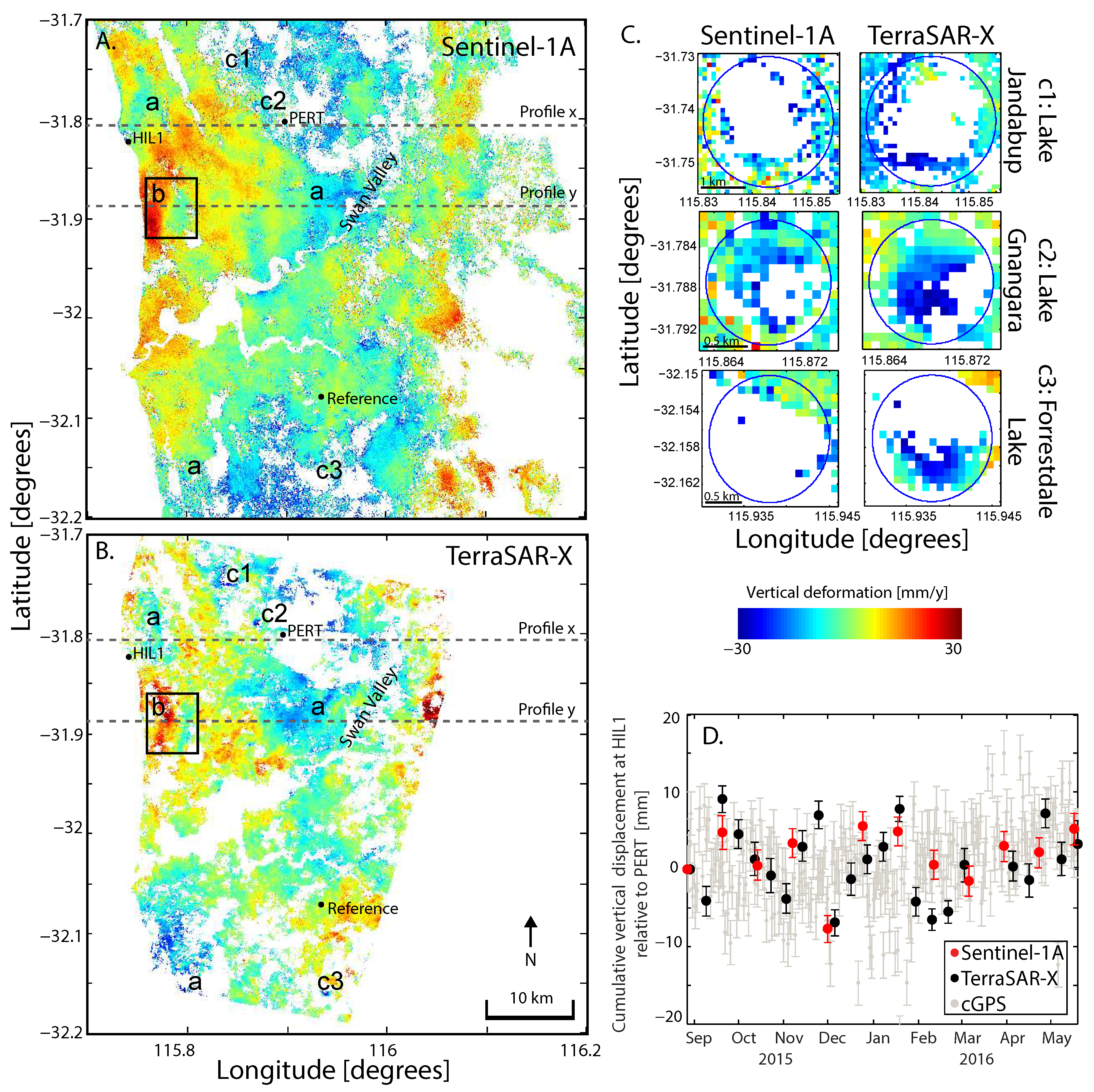
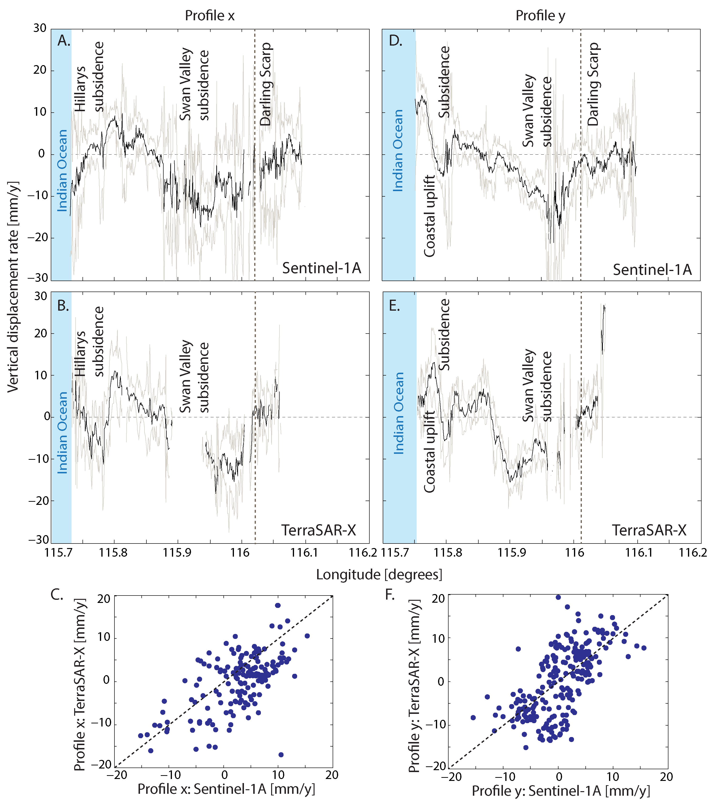
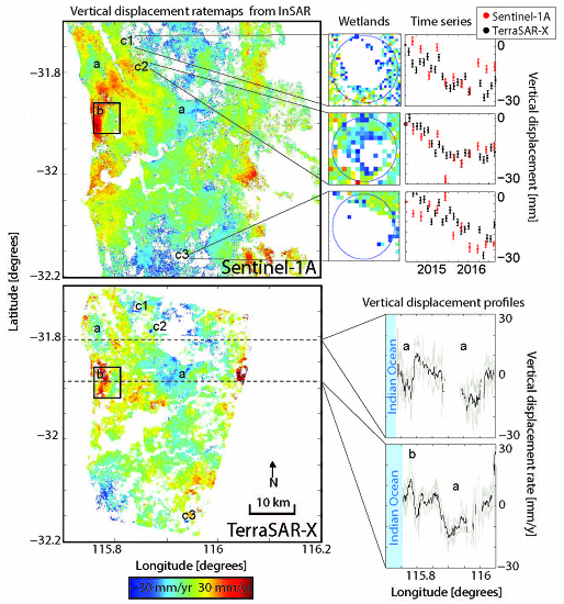
5.2.1. Broad-Scale, Slow Subsidence

Broad (>5 km wide) subsidence relative to the reference region that is common to both sets of satellite images is observed in three locations: proximal to Hillarys, through the Swan Valley and south of Fremantle (labelled (a) in Figure 4A,B). Whilst subsidence proximal to Hillarys has been identified in past deformation studies in the Perth Basin [1], displacements in the Swan Valley and south of Fremantle have not previously been detected due to the limited spatial coverage of historical datasets [8].

The signal south of Fremantle is offset in latitude between datasets: the maximum displacements for Sentinel-1A are beyond the extent of the TerraSAR-X scene, and it is therefore difficult to draw a profile through the signal in both datasets. Broad subsidence through Hillarys and the Swan Valley is shown by displacement profile x (Figure 4 and Figure 5A,B). Displacement rates proximal to Hillarys reach 7 mm/y to 10 mm/y, with the maximum magnitude of deformation ∼3 km east of the coast in the TerraSAR-X dataset. The profile shows that subsidence through the Swan Valley occurs over a wider area with displacements rates up to ∼15 mm/y over the observation period. At the eastern end of the profile, both datasets show correlation with the location of the Darling Scarp, likely due to residual stratified atmospheric noise. Plotting the values of profile x for Sentinel-1A against those for TerraSAR-X demonstrates general agreement between the two datasets with a correlation coefficient of 0.67 (Figure 5C). Scatter may be partly attributed to differences in the satellite look angle, the different times of the satellite acquisitions and associated variations in uncorrected atmospheric delay.

5.2.2. Adjacent Uplift and Subsidence

South of Hillarys, contrasting, but adjacent regions of relative uplift and subsidence are identified in both the Sentinel-1A and TerraSAR-X deformation rate-maps and are shown by the rectangle labelled (b) in Figure 4A,B. Displacement profile y (Figure 4 and Figure 5D,E) shows this transition from positive to negative displacement, recording maximum rates of ∼+15 mm/y and ∼−7 mm/y, respectively. This contrast between adjacent positive and negative displacements may be indicative of a barrier to flow in the groundwater system, such as a permeability contrast or unmapped fault [78]. Profile y also reveals a slight offset in the maximum displacement between the two datasets, which may be attributed to differences in the line of sight direction of each satellite or residual quasi-systematic atmospheric banding in the Sentinel-1A dataset in this part of the image (Figure 4A). Assessing the correlation between profile y from Sentinel-1A and TerraSAR-X shows that, whilst the results are largely similar, the magnitudes of displacements from TerraSAR-X tend to be ∼10% larger (Figure 5F).

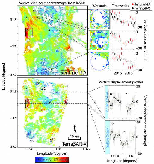
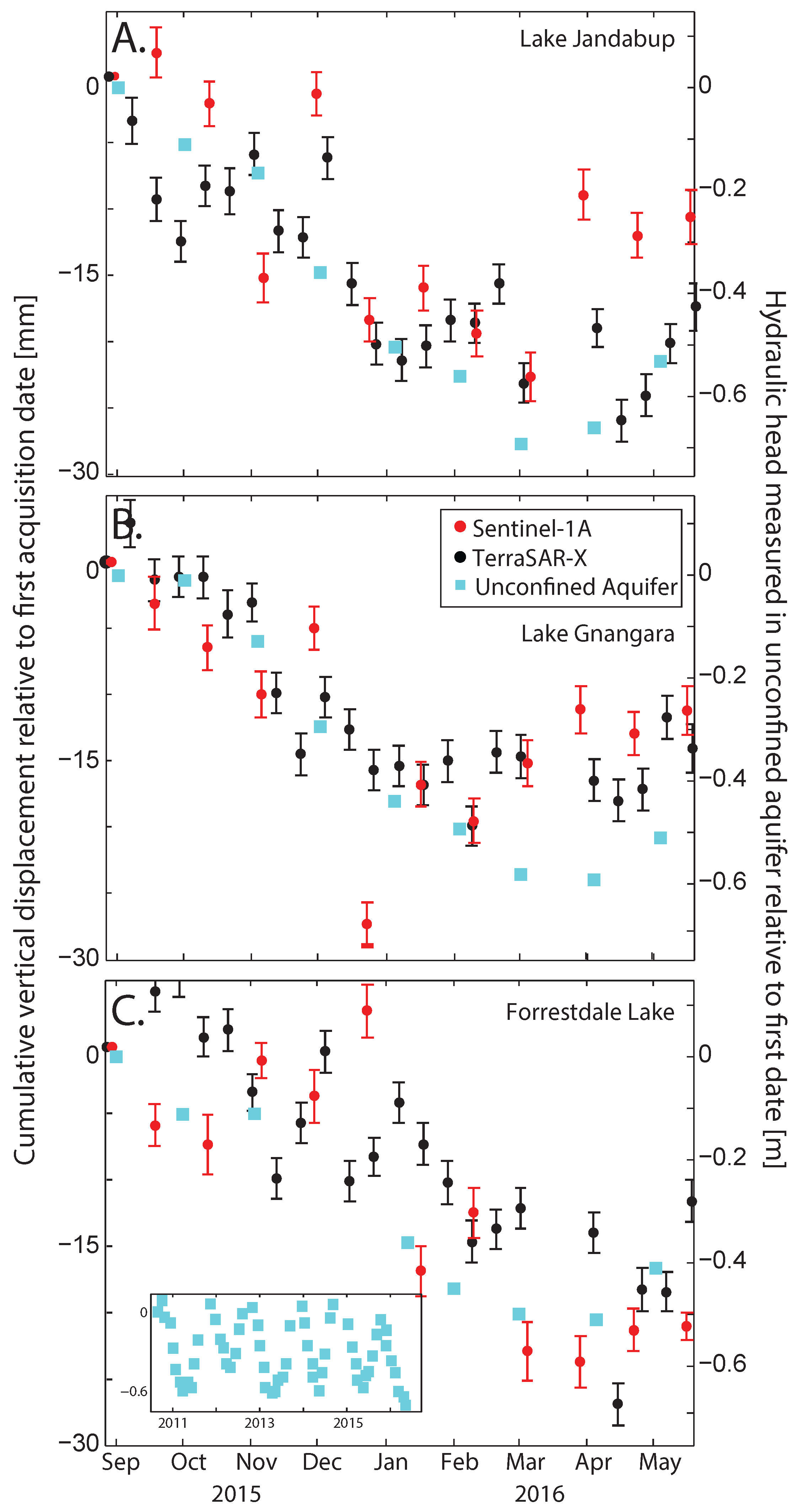
5.2.3. Seasonal Deformation Coincident with Wetland Areas

Subsidence of 20–25 mm/y is identified in three regions over the 0.7-y observation period: Lake Jandabup, Lake Gnangara and Forrestdale Lake (labelled (c1, c2, c3) in Figure 4C, respectively). In each case, displacements are confined to a region up to 2 km wide and are coincident with wetland areas. We investigate these signals using time series of cumulative displacements. Time series from TerraSAR-X and Sentinel-1A show comparable results, although overall, the higher acquisition frequency of TerraSAR-X better captures changes in deformation over time (Figure 6). Where acquisitions from the two satellites are separated by less than three days, we directly compare the Sentinel-1A measurements to TerraSAR-X. In cases where the temporal offset is greater, we compare the Sentinel-1A result to the average of the two closest TerraSAR-X acquisitions. The mean difference between the two datasets is ∼5 mm at Lake Jandabup and Forrestdale Lake and ∼3 mm at Lake Gnangara, which in all cases is at least three-times smaller than the magnitude of the maximum displacement measured over the observation period (Figure 6).

The temporal evolution of cumulative displacements at all three wetland areas is similar, and we compare the InSAR time series to changes in hydraulic head in the unconfined aquifer measured at nearby artesian monitoring bores and obtained from the Western Australian Department of Water (Section 3). The groundwater data in Figure 6 are the average of hydraulic head measured at all bores within 3 km of each wetland. Groundwater level data and InSAR displacements show close agreement over time (Figure 6), confirming that the InSAR measurements capture surface changes correlated with seasonal variations in hydraulic head [79]. Hydraulic head and ground displacements decrease between the first acquisition in late August 2015 and late March 2016, coincident with the Southern Hemisphere spring and summer months and the period of low rainfall in the Perth region (Figure 6). The signal then begins to reverse, most notably at Lake Jandabup (Figure 6A), with increasing water levels and positive or neutral ground displacement. The maximum relative subsidence is ∼23 mm at Lake Jandabup, ∼20 mm at Lake Gnangara and ∼24 mm at Forrestdale Lake. At Lake Jandabup, there is ∼7 mm of relative uplift that occurs between March and the time of the last acquisition in May.

Lake Jandabup, Lake Gnangara and Forrestdale Lake are located within clay/swamp surface deposits (Figure 2). Clays, silts and other poorly consolidated sediments are fine-grained and highly compressible, and therefore, subsidence in the unconfined aquifer is most likely to be coincident with these deposits [43]. Displacements may also arise due to shallow (top metre) shrinkage and swelling of the deposits in response to changes in water content [80]. However, it is not immediately evident why the three wetland/swamp regions identified in Figure 4 exhibit subsidence, whereas others do not, despite being associated with the same surface geology. We calculate displacement time series at five other wetland areas throughout the Perth Basin, but all show cumulative displacements of less than 5 mm over the observation period, despite changes in hydraulic head at nearby wells comparable to those shown in Figure 6. This disparity may be linked to variations in hydraulic conductivity between wetland areas and the unconfined aquifer or the occurrence/absence of sediments that are more susceptible to seasonal swelling and shrinkage. Other factors found to control the spatial distribution of deformation include the distribution of extraction wells, the thickness of deposits [77] and the presence of barriers to groundwater flow [81].

6. Future Monitoring of the Perth Basin

InSAR data are being used increasingly to complement or replace ground-based geodetic surveys for deformation monitoring due to a broader spatial coverage and lower costs. Applying these data to the Perth Basin, we have been able to investigate a larger spatial extent of the deformation field, albeit over a limited time interval (0.7 y) that was solely governed by the availability of Sentinel-1A data. Whilst it is not possible to determine whether the displacements we have measured are representative of long-term deformation or are seasonal variations, the observations do indeed provide new insights into the spatial distribution of ground displacements in the Perth Basin that can be used to coordinate subsequent focused subsidence monitoring over targeted regions [2].

To guide future InSAR studies in the Perth Basin, we estimate the time period required to measure subsidence at linear rates obtained from previous time series analysis at GPS stations HIL1 and PERT [1] using Sentinel-1 and TerraSAR-X. Between 1994/1998 and 2012, time series at the two GPS stations show non-linear subsidence that correlates with groundwater levels from the deeper Leederville and Yarragadee aquifers [1]. After removal of annual and semi-annual seasonal signals, this was modelled by three piecewise linear trends spanning 1994/1998–2000, 2000–2005 and 2005–2012 (

Table 1. Number of satellite acquisitions and corresponding period of time required to measure past vertical deformation rates at continuous GPS stations PERT and HIL1 not accounting for seasonal effects.

	PERT			HIL1
Epoch	1994–2000	2000–2005	2005–2012	1998–2000	2000–2005	2005–2012
Subsidence rate (mm/y) ${}^a$	0.90 ± 1.97	5.42 ± 2.36	2.51 ± 1.89	6.56 ± 2.69	6.97 ± 1.30	3.12 ± 0.92
Sentinel-1A acquisition strategy for data in this study (every other cycle: 24-day repeat)
Acquisitions (years)	32 (2.10 y)	16 (1.05 y)	21 (1.38 y)	14 (0.92 y)	14 (0.92 y)	19 (1.25 y)
Sentinel-1B acquisition strategy implemented since November 2016 (12-day repeat)
Acquisitions (years)	55 (1.81 y)	27 (0.89 y)	37 (1.21 y)	25 (0.82 y)	24 (0.78 y)	33 (1.08 y)
Sentinel-1A/B acquisition strategy over Europe (6-day repeat)
Acquisitions (years)	96 (1.58 y)	47 (0.77 y)	64 (1.05 y)	43 (0.71 y)	42 (0.69 y)	58 (0.95 y)
TerraSAR-X (11-day repeat)
Acquisitions (years)	47 (1.40 y)	23 (0.69 y)	31 (0.98 y)	21 (0.63 y)	21 (0.63 y)	28 (0.84 y)

${}^a$ Piecewise linear vertical deformation rates from Table 2 in Featherstone et al. [1].

). The largest subsidence rate (6.97 ± 1.30 mm/y) was at HIL1 between 2000 and 2005. The smallest reliable GPS rate (i.e., that with an estimated error smaller than the estimated rate) (2.51 ± 1.89 mm/y) was at PERT between 2005 and 2012 [1].

For each of the GPS epochs, we estimate the error on InSAR measurements using the method described in Parker et al. [60]. This takes into consideration the length of the observation period, the frequency of the acquisitions and the standard deviation of the atmospheric noise. We estimate the standard deviation of the atmospheric noise by masking the regions identified to be deforming in Figure 4A,B and assuming that residual phase signals are due to uncorrected atmospheric noise. The average standard deviation of the ERA-I corrected interferograms is ∼9 mm for Sentinel-1A and ∼5 mm for TerraSAR-X. For each satellite mission, we assume there are no gaps in acquisitions. We include results for Sentinel-1A at the acquisition frequency of data in this study (24-day repeat intervals), the acquisition frequency implemented for Sentinel-1B since October 2016 (12-day repeat intervals) and the current combined Sentinel-1A and -1B acquisition frequency over Europe (six-day repeat intervals) assuming the same value of atmospheric noise. In each case, we consider subsidence to be detectable when the cumulative deformation exceeds the estimated error.

The results for each GPS epoch are shown in Table 1. Over the period of this study (0.7 y), TerraSAR-X may be able to detect deformation at HIL1 and PERT at the 2000–2005 rates and at HIL1 at the 1998–2000 rate. However, neither TerraSAR-X nor Sentinel-1A are able to detect deformation at the smaller 2005–2012 rates at PERT or HIL1, with Sentinel-1A requiring 1.38 years to detect the smallest magnitude signal identified by Featherstone et al. [1] at PERT. This is approximately double the current period of continuous Sentinel-1A acquisitions over the Perth Basin. For the newly-implemented Sentinel-1B acquisition strategy (12-day intervals), the estimated detection periods reduce by an average of 14% (Table 1). In the case of Sentinel-1A and -1B at six-day repeat intervals, the theoretical detection period decreases by 25%. At this level of repeat, the results suggest that Sentinel-1 may detect deformation at both HIL1 and PERT at the 2000–2005 rates over the period of this study.

Estimating the minimum observation length or repeat frequency to measure small-magnitude deformation in this way is informative for planning future monitoring strategies. Whilst the method is transferable to other settings, in practice, the results may underestimate the time required to accurately measure multi-year deformation rates, as we have not accounted for seasonal and other non-linear effects. Studies of annually varying signals in GPS time series suggest that 2–3 years of data are required to characterise and remove the seasonal component and avoid biasing the long-term velocity estimate [82,83]. Such non-linear seasonal signals are better characterised with acquisitions at higher temporal resolution, as shown by the time series in Figure 6, and would therefore be best measured at the full repeat of Sentinel-1A and -1B. Identifying and measuring small, non-linear, seasonal and broad-scale subsidence/uplift such as that in the Perth Basin is also complicated by the shape of the deformation signals, which are not necessarily spatially distinguishable from atmospheric phase features [75] and, unlike other geophysical phenomena, such as the characteristic “bullseye” associated with volcanic inflation [84], do not necessarily occur in a predictable way (e.g., patchy subsidence: [54,77]) (Figure 4).

The results of this study demonstrate that, even over the short 0.7-y observation period, Sentinel-1A acquisitions over the Perth Basin have provided improved information about the larger spatial extent of deformation. However, the results in Table 1 show the benefit of the newly-implemented, higher-frequency Sentinel-1B acquisition strategy, which is planned to continue for longer than the duration of the Sentinel-1A dataset and the required detection periods calculated in Table 1 [26]. With this longer time series of data, we will be better equipped to robustly measure subsidence throughout the Perth Basin, firstly confirming whether, in addition to Hillarys, the areas south of Fremantle and in the Swan Valley are undergoing broad-scale, long-term subsidence and, secondly, differentiating between seasonal and long-term displacements in order to constrain the elastic and inelastic storage properties of the regional aquifers [2].

7. Conclusions

Previous ground-based geodetic surveys have revealed subsidence at discrete points or along traverses in parts of the Perth Basin, but these measurements are spatially limited and sample only a small part of the metropolitan area. We have therefore carried out an investigation into the broader extent of the deformation field by performing the first application of Sentinel-1A InSAR data to Australia from published literature to date. Whilst the observation period is short (0.7 y), verification of Sentinel-1A with independent TerraSAR-X and continuous GPS (a) demonstrates close agreement between the vertical displacement fields measured with each satellite, acknowledging the effects of unmodelled atmospheric noise; and (b) provides new insights into the broader deformation field of the Perth Basin that can be used to guide subsequent targeted studies.

With both Sentinel-1A and TerraSAR-X, we observe broad regions (>5 km wide) of small-magnitude (up to 15 mm/y) relative subsidence at Hillarys, through the agricultural Swan Valley and a region south of Fremantle. Other displacements are observed in elongated zones of adjacent relative uplift and subsidence south of Hillarys, and regions of relative subsidence at higher rates (greater than 20 mm/y), but on a smaller scales (∼2 km wide), are found to be coincident with wetland areas. At these wetlands, time series of cumulative ground displacements are further verified by measurements of hydraulic head in the unconfined aquifer.

Overall, these observations demonstrate the ability of Sentinel-1A to detect small-magnitude deformation over different spatial scales (from 2 km–10 s of km) in the Perth Basin. However, ongoing acquisitions of Sentinel-1B data are key to better characterising seasonal and long-term deformation rates. These measurements may provide useful constraints upon the hydromechanical structure of the Perth Basin aquifer system, which supports wetlands, agriculture, industry and a population of over two million people [85].

References

1. Featherstone, W.E.; Penna, N.T.; Filmer, M.S.; Williams, S.D.P. Nonlinear subsidence at Fremantle, a long-recording tide gauge in the Southern Hemisphere. J. Geophys. Res. 2015, 120, 7004–7014. [Google Scholar] [CrossRef]
2. Galloway, D.L.; Burbey, T.J. Review: Regional land subsidence accompanying groundwater extraction. Hydrogeol. J. 2011, 19, 1459–1486. [Google Scholar] [CrossRef]
3. Bruun, P. The Bruun rule of erosion by sea-level rise: A discussion on large-scale two-and three-dimensional usages. J. Coast. Res. 1988, 4, 627–648. [Google Scholar]
4. Dixon, T.H.; Amelung, F.; Ferretti, A.; Novali, F.; Rocca, F.; Dokka, R.; Sella, G.; Kim, S.-W.; Wdowinski, S.; Whitman, D. Space geodesy: Subsidence and flooding in New Orleans. Nature 2006, 441, 587–588. [Google Scholar] [CrossRef] [PubMed]
5. Phien-Wej, N.; Giao, P.H.; Nutalaya, P. Land subsidence in Bangkok, Thailand. Eng. Geol. 2006, 82, 187–201. [Google Scholar] [CrossRef]
6. Brooks, B.A.; Merrifield, M.A.; Foster, J.; Werner, C.L.; Gomez, F.; Bevis, M.; Gill, S. Space geodetic determination of spatial variability in relative sea level change, Los Angeles basin. Geophys. Res. Lett. 2007, 34. [Google Scholar] [CrossRef]
7. Bell, J.W.; Amelung, F.; Ferretti, A.; Bianchi, M.; Novali, F. Permanent scatterer InSAR reveals seasonal and long-term aquifer-system response to groundwater pumping and artificial recharge. Water Resour. Res. 2008, 44. [Google Scholar] [CrossRef]
8. Featherstone, W.E.; Filmer, M.S.; Penna, N.T.; Morgan, L.M.; Schenk, A. Anthropogenic land subsidence in the Perth Basin: Challenges for its retrospective geodetic detection. J. R. Soc. West. Aust. 2012, 95, 53–62. [Google Scholar]
9. Vanicek, P.; Castle, R.O.; Balazs, E.I. Geodetic leveling and its applications. Rev. Geophys. 1980, 18, 505–524. [Google Scholar] [CrossRef]
10. Wang, T.; Perissin, D.; Rocca, F.; Liao, M.-S. Three Gorges Dam stability monitoring with time series InSAR image analysis. Sci. China Earth Sci. 2011, 54, 720–732. [Google Scholar] [CrossRef]
11. Pritchard, M.E.; Simons, M. Surveying volcanic arcs with satellite radar interferometry: The Central Andes, Kamchatka, and beyond. GSA Today 2004, 14, 4–11. [Google Scholar] [CrossRef]
12. Bürgmann, R.; Rosen, P.A.; Fielding, E.J. Synthetic aperture radar interferometry to measure Earth’s surface topography and its deformation. Annu. Rev. Earth Planet. Sci. 2000, 28, 169–209. [Google Scholar] [CrossRef]
13. Hanssen, R.F. Radar Interferometry: Data Interpretation and Analysis; Kluwer Acad.: Norwell, MA, USA, 2001. [Google Scholar]
14. Massonnet, D.; Feigl, K.L. Radar interferometry and its application to changes in the Earth’s surface. Rev. Geophys. 1998, 36, 441–500. [Google Scholar] [CrossRef]
15. Simons, M.; Rosen, P.A. Interferometric synthetic aperture radar geodesy. In Treatise on Geophysics—Geodesy; Elsevier: Amsterdam, The Netherlands, 2007; Volume 3, pp. 391–446. [Google Scholar]
16. Ng, A.H.-M.; Ge, L. Application of persistent scatterer InSAR and GIS for urban subsidence monitoring. In Proceedings of the 2007 IEEE International Geoscience and Remote Sensing Symposium, Barcelona, Spain, 23–28 July 2007; pp. 1091–1094.
17. Dawson, J. Satellite Radar Interferometry with Application to the Observation of Surface Deformation in Australia. Ph.D. Thesis, The Australian National University, Canberra, Australia, 2008. [Google Scholar]
18. Torres, R.; Snoeij, P.; Geudtner, D.; Bibby, D.; Davidson, M.; Attema, E.; Potin, P.; Rommen, B.; Floury, N.; Brown, M.; et al. GMES Sentinel-1 mission. Remote Sens. Environ. 2012, 120, 9–24. [Google Scholar] [CrossRef]
19. Diao, F.; Walter, T.R.; Motagh, M.; Prats-Iraola, P.; Wang, R.; Samsonov, S.V. The 2015 Gorkha earthquake investigated from radar satellites: Slip and stress modeling along the MHT. Front. Earth Sci. 2015. [Google Scholar] [CrossRef]
20. Elliott, J.R.; Jolivet, R.; González, P.J.; Avouac, J.-P.; Hollingsworth, J.; Searle, M.P.; Stevens, V.L. Himalayan megathrust geometry and relation to topography revealed by the Gorkha earthquake. Nat. Geosci. 2016, 9, 174–180. [Google Scholar] [CrossRef]
21. Grandin, R.; Vallée, M.; Satriano, C.; Lacassin, R.; Klinger, Y.; Simoes, M.; Bollinger, L. Rupture process of the Mw = 7.9 2015 Gorkha earthquake (Nepal): Insights into Himalayan megathrust segmentation. Geophys. Res. Lett. 2015, 42, 8373–8382. [Google Scholar] [CrossRef]
22. Sreejith, K.M.; Sunil, P.S.; Agrawal, R.; Saji, A.P.; Ramesh, D.S.; Rajawat, A.S. Coseismic and early postseismic deformation due to the 25 April 2015, Mw 7.8 Gorkha, Nepal, earthquake from InSAR and GPS measurements. Geophys. Res. Lett. 2016, 43, 3160–3168. [Google Scholar]
23. González, P.J.; Bagnardi, M.; Hooper, A.J.; Larsen, Y.; Marinkovic, P.; Samsonov, S.V.; Wright, T.J. The 2014–2015 eruption of Fogo volcano: Geodetic modeling of Sentinel-1 TOPS interferometry. Geophys. Res. Lett. 2015, 42, 9239–9246. [Google Scholar] [CrossRef]
24. Kim, J.-W.; Lu, Z.; Degrandpre, K. Ongoing deformation of sinkholes in Wink, Texas, observed by time series Sentinel-1A SAR interferometry (preliminary results). Remote Sens. 2016, 8, 313. [Google Scholar] [CrossRef]
25. Giardini, D.; Grünthal, G.; Shedlock, K.M.; Zhang, P. The GSHAP global seismic hazard map. Ann. Geophys. 1999, 42. [Google Scholar] [CrossRef]
26. Copernicus Space Component Mission Management Team. Sentinel High Level Operations Plan; Tech. Rep. COPE-S1OP-EOPG-PL-0020; European Space Agency: Paris, France, 2015. [Google Scholar]
27. McCue, K. Australia’s large earthquakes and Recent fault scarps. J. Struct. Geol. 1990, 12, 761–766. [Google Scholar] [CrossRef]
28. Brown, A.; Gibson, G. A multi-tiered earthquake hazard model for Australia. Tectonophysics 2004, 390, 25–43. [Google Scholar] [CrossRef]
29. Dawson, J.; Tregoning, P. Uncertainty analysis of earthquake source parameters determined from InSAR: A simulation study. J. Geophys. Res. 2007, 112. [Google Scholar] [CrossRef]
30. Dawson, J.; Cummins, P.; Tregoning, P.; Leonard, M. Shallow intraplate earthquakes in Western Australia observed by Interferometric Synthetic Aperture Radar. J. Geophys. Res. 2008, 113. [Google Scholar] [CrossRef]
31. Ge, L.; Ng, A.H.-M.; Wang, H.; Rizos, C. Crustal deformation in Australia measured by satellite radar interferometry using ALOS/PALSAR imagery. J. Appl. Geod. 2009, 3, 47–53. [Google Scholar]
32. Ng, A.H.-M.; Ge, L.; Yan, Y.; Li, X.; Chang, H.-C.; Zhang, K.; Rizos, C. Mapping accumulated mine subsidence using small stack of SAR differential interferograms in the Southern coalfield of New South Wales, Australia. Eng. Geol. 2010, 115, 1–15. [Google Scholar] [CrossRef]
33. Ng, A.H.-M.; Ge, L.; Zhang, K.; Chang, H.-C.; Li, X.; Rizos, C.; Omura, M. Deformation mapping in three dimensions for underground mining using InSAR- Southern highland coalfield in New South Wales, Australia. Int. J. Remote Sens. 2011, 32, 7227–7256. [Google Scholar] [CrossRef]
34. Ng, A.H.-M.; Ge, L.; Zhang, K.; Li, X. Estimating horizontal and vertical movements due to underground mining using ALOS PALSAR. Eng. Geol. 2012, 143, 18–27. [Google Scholar] [CrossRef]
35. Iannacone, J.P.; Corsini, A.; Berti, M.; Morgan, J.; Falorni, G. Characterization of Longwall Mining Induced Subsidence by Means of Automated Analysis of InSAR Time-Series. In Engineering Geology for Society and Territory; Springer: Berlin/Heidelberg, Germany, 2015; Volume 5, pp. 973–977. [Google Scholar]
36. Du, Z.; Ge, L.; Li, X.; Ng, A.H.-M. Subsidence Monitoring over the Southern Coalfield, Australia Using both L-Band and C-Band SAR Time Series Analysis. Remote Sens. 2016, 8, 543. [Google Scholar] [CrossRef]
37. Ng, A.H.-M.; Ge, L.; Li, X. Assessments of land subsidence in the Gippsland Basin of Australia using ALOS PALSAR data. Remote Sens. Environ. 2015, 159, 86–101. [Google Scholar] [CrossRef]
38. Moghaddam, N.F.; Samsonov, S.V.; Rüdiger, C.; Walker, J.P.; Hall, W.D.M. Multi-temporal SAR observations of the Surat Basin in Australia for deformation scenario evaluation associated with man-made interactions. Environ. Earth Sci. 2016, 75, 1–16. [Google Scholar] [CrossRef]
39. Garthwaite, M.C.; Hazelwood, M.; Nancarrow, S.; Hislop, A.; Dawson, J. A regional geodetic network to monitor ground surface response to resource extraction in the northern Surat Basin, Queensland. Aust. J. Earth Sci. 2015, 62, 469–477. [Google Scholar] [CrossRef]
40. Playford, P.E.; Low, G.H.; Cockbain, A.E. Geology of the Perth Basin, Western Australia; Geological Survey of Western Australia: Perth, Australia, 1976.
41. Lambeck, K. The Perth Basin: A possible framework for its formation and evolution. Explor. Geophys. 1987, 18, 124–128. [Google Scholar] [CrossRef]
42. Dentith, M.C.; Bruner, I.; Long, A.; Middleton, M.F.; Scott, J. Structure of the eastern margin of the Perth Basin, Western Australia. Explor. Geophys. 1993, 24, 455–462. [Google Scholar] [CrossRef]
43. Davidson, W.A. Hydrogeology and Groundwater Resources of the Perth Region, Western Australia; Geological Survey of Western Australia: Perth, Australia, 1995.
44. Rosen, P.A.; Gurrola, E.; Sacco, G.F.; Zebker, H. The InSAR scientific computing environment. In Proceedings of the 9th European Conference on Synthetic Aperture Radar (EUSAR 2012), Nürnberg, Germany, 23–26 April 2012; pp. 730–733.
45. Parker, A.L.; Biggs, J.; Lu, Z. Investigating long-term subsidence at Medicine Lake Volcano, CA, using multi temporal InSAR. Geophys. J. Int. 2014, 199, 844–859. [Google Scholar]
46. Miranda, N. Sentinel-1 Instrument Processing Facility: Impact of the Elevation Antenna Pattern Phase Compensation on the Interferometric Phase Preservation; Tech. Rep. ESA-EOPG-CSCOP-TN-0004; European Space Agency: Paris, France, 2015. [Google Scholar]
47. Gallant, J.C.; Dowling, T.I.; Read, A.M.; Wilson, N.; Tickle, P.; Inskeep, C. 1 Second SRTM Derived Digital Elevation Models User Guide. 2011. Available online: http://www.ga.gov.au/topographic-mapping/digital-elevation-data.html (accessed on 28 August 2016). [Google Scholar]
48. Sansosti, E.; Berardino, P.; Manunta, M.; Serafino, F.; Fornaro, G. Geometrical SAR image registration. IEEE Trans. Geosci. Remote Sens. 2006, 44, 2861–2870. [Google Scholar]
49. Prats-Iraola, P.; Scheiber, R.; Marotti, L.; Wollstadt, S.; Reigber, A. TOPS interferometry with TerraSAR-X. IEEE Trans. Geosci. Remote Sens. 2012, 50, 3179–3188. [Google Scholar] [CrossRef] [Green Version]
50. Yagüe-Martínez, N.; Prats-Iraola, P.; Gonzalez, F.R.; Brcic, R.; Shau, R.; Geudtner, D.; Eineder, M.; Bamler, R. Interferometric processing of Sentinel-1 TOPS Data. IEEE Trans. Geosci. Remote Sens. 2016, 54, 2220–2234. [Google Scholar] [CrossRef]
51. Goldstein, R.; Werner, C. Radar interferogram filtering for geophysical applications. Geophys. Res. Lett. 1998, 25, 4035–4038. [Google Scholar]
52. Chen, C.W.; Zebker, H.A. Network approaches to two-dimensional phase unwrapping: Intractability and two new algorithms. J. Opt. Soc. Am. A 2000, 17, 401–414. [Google Scholar] [CrossRef]
53. Jónsson, S.; Zebker, H.; Segall, P.; Amelung, F. Fault slip distribution of the 1999 Mw 7.1 Hector Mine, California, earthquake, estimated from satellite radar and GPS measurements. Bull. Seismol. Soc. Am. 2002, 92, 1377–1389. [Google Scholar] [CrossRef]
54. Chaussard, E.; Amelung, F.; Abidin, H.; Hong, S.-H. Sinking cities in Indonesia: ALOS PALSAR detects rapid subsidence due to groundwater and gas extraction. Remote Sens. Environ. 2013, 128, 150–161. [Google Scholar] [CrossRef]
55. Wright, T.J.; Parsons, B.E.; Lu, Z. Toward mapping surface deformation in three dimensions using InSAR. Geophys. Res. Lett. 2004, 31. [Google Scholar] [CrossRef]
56. Biggs, J.; Wright, T.; Lu, Z.; Parsons, B. Multi-interferogram method for measuring interseismic deformation: Denali Fault, Alaska. Geophys. J. Int. 2007, 170, 1165–1179. [Google Scholar] [CrossRef]
57. Zebker, H.A.; Rosen, P.A.; Hensley, S. Atmospheric effects in interferometric synthetic aperture radar surface deformation and topographic maps. J. Geophys. Res. 1997, 102, 7547–7563. [Google Scholar] [CrossRef]
58. Doin, M.-P.; Lasserre, C.; Peltzer, G.; Cavalié, O.; Doubre, C. Corrections of stratified tropospheric delays in SAR interferometry: Validation with global atmospheric models. J. Appl. Geophys. 2009, 69, 35–50. [Google Scholar] [CrossRef]
59. Emardson, T.R.; Simons, M.; Webb, F.H. Neutral atmospheric delay in interferometric synthetic aperture radar applications: Statistical description and mitigation. J. Geophys. Res. 2003, 108. [Google Scholar] [CrossRef]
60. Parker, A.L.; Biggs, J.; Walters, R.J.; Ebmeier, S.K.; Wright, T.J.; Teanby, N.A.; Lu, Z. Systematic assessment of atmospheric uncertainties for InSAR data at volcanic arcs using large-scale atmospheric models: Application to the Cascade volcanoes, United States. Remote Sens. Environ. 2015, 170, 102–114. [Google Scholar] [CrossRef]
61. Elliott, J.R.; Biggs, J.; Parsons, B.; Wright, T.J. InSAR slip rate determination on the Altyn Tagh Fault, northern Tibet, in the presence of topographically correlated atmospheric delays. Geophys. Res. Lett. 2008, 35. [Google Scholar] [CrossRef]
62. Lin, Y.N.; Simons, M.; Hetland, E.A.; Muse, P.; DiCaprio, C. A multiscale approach to estimating topographically correlated propagation delays in radar interferograms. Geochem. Geophys. Geosyst. 2010, 11, 5424–5425. [Google Scholar] [CrossRef]
63. Jolivet, R.; Agram, P.S.; Lin, N.Y.; Simons, M.; Doin, M.-P.; Peltzer, G.; Li, Z. Improving InSAR geodesy using global atmospheric models. J. Geophys. Res. 2014, 119, 2324–2341. [Google Scholar] [CrossRef]
64. Williams, S.; Bock, Y.; Fang, P. Integrated satellite interferometry: Tropospheric noise, GPS estimates and implications for interferometric synthetic aperture radar products. J. Geophys. Res. 1998, 103, 27051–27067. [Google Scholar] [CrossRef]
65. Yu, C.; Penna, N.T.; Li, Z. Generation of real-time mode high-resolution water vapor fields from GPS observations. J. Geophys. Res. 2017, 122, 2008–2025. [Google Scholar] [CrossRef]
66. Jolivet, R.; Grandin, R.; Lasserre, C.; Doin, M.-P.; Peltzer, G. Systematic InSAR tropospheric phase delay corrections from global meteorological reanalysis data. Geophys. Res. Lett. 2011, 38. [Google Scholar] [CrossRef] [Green Version]
67. Walters, R.J.; Elliott, J.R.; Li, Z.; Parsons, B. Rapid strain accumulation on the Ashkabad fault (Turkmenistan) from atmosphere-corrected InSAR. J. Geophys. Res. 2013, 118, 3674–3690. [Google Scholar] [CrossRef]
68. Dee, D.P.; Uppala, S.M.; Simmons, A.J.; Berrisford, P.; Poli, P.; Kobayashi, S.; Andrae, U.; Balmaseda, M.A.; Balsamo, G.; Bauer, P.; et al. The ERA-Interim reanalysis: Configuration and performance of the data assimilation system. Q. J. R. Meteorol. Soc. 2011, 137, 553–597. [Google Scholar]
69. Uppala, S.; Dee, D.; Kobayashi, S.; Berrisford, P.; Simmons, A. Towards a climate dataassimilation system: Status update of ERA-Interim. ECMWF Newslett. 2008, 115, 12–18. [Google Scholar]
70. Simmons, A.; Uppala, S.; Dee, D.; Kobayashi, S. ERA-Interim: New ECMWF reanalysis products from 1989 onwards. ECMWF Newslett. 2007, 110, 25–35. [Google Scholar]
71. Gourmelen, N.; Amelung, F.; Lanari, R. Interferometric synthetic aperture radar-GPS integration: Interseismic strain accumulation across the Hunter Mountain fault in the eastern California shear zone. J. Geophys. Res. 2010, 115. [Google Scholar] [CrossRef]
72. Davidson, W.A.; Yu, X. Perth Regional Aquifer Modelling System (PRAMS) Model Development: Hydrogeology and Groundwater Modelling; Western Australia Department of Water: Perth, Western Australia, Australia, 2008.
73. Lundgren, P.; Usai, S.; Sansosti, E.; Lanari, R.; Tesauro, M.; Fornaro, G.; Berardino, P. Modeling surface deformation observed with synthetic aperture radar interferometry at Campi Flegrei caldera. J. Geophys. Res. 2001, 106, 19355–19366. [Google Scholar]
74. Berardino, P.; Fornaro, G.; Lanari, R.; Sansosti, E. A new algorithm for surface deformation monitoring based on small baseline differential SAR interferograms. IEEE Trans. Geosci. Remote Sens. 2002, 40, 2375–2383. [Google Scholar] [CrossRef]
75. Ebmeier, S.K.; Biggs, J.; Mather, T.A.; Amelung, F. On the lack of InSAR observations of magmatic deformation at Central American volcanoes. J. Geophys. Res. 2013, 118, 2571–2585. [Google Scholar] [CrossRef]
76. Li, Z.; Fielding, E.J.; Cross, P.; Muller, J.-P. Interferometric synthetic aperture radar atmospheric correction: GPS topography-dependent turbulence model. J. Geophys. Res. 2006, 111. [Google Scholar] [CrossRef]
77. Chaussard, E.; Wdowinski, S.; Cabral-Cano, E.; Amelung, F. Land subsidence in central Mexico detected by ALOS InSAR time series. Remote Sens. Environ. 2014, 140, 94–106. [Google Scholar] [CrossRef]
78. Cabral-Cano, E.; Osmanoglu, B.; Dixon, T.; Wdowinski, S.; DeMets, C.; Cigna, F.; Díaz-Molina, O. Subsidence and fault hazard maps using PSI and permanent GPS networks in central Mexico. In Proceedings of the Eighth International Symposium on Land Subsidence, Querétaro, Mexico, 17–22 October 2010; pp. 17–22.
79. Reeves, J.A.; Knight, R.; Zebker, H.A.; Schreüder, W.A.; Agram, P.; Lauknes, T.R. High quality InSAR data linked to seasonal change in hydraulic head for an agricultural area in the San Luis Valley, Colorado. Water Resour. Res. 2011, 47. [Google Scholar] [CrossRef]
80. Gabriel, A.K.; Goldstein, R.M.; Zebker, H.A. Mapping small elevation changes over large areas: Differential radar interferometry. J. Geophys. Res. 1989, 94, 9183–9191. [Google Scholar] [CrossRef]
81. Hoffmann, J.; Zebker, H.A.; Galloway, D.L.; Amelung, F. Seasonal subsidence and rebound in Las Vegas Valley, Nevada, observed by synthetic aperture radar interferometry. Water Resour. Res. 2001, 37, 1551–1566. [Google Scholar] [CrossRef]
82. Blewitt, G.; Lavallée, D. Effect of annual signals on geodetic velocity. J. Geophys. Res. 2002, 107. [Google Scholar] [CrossRef]
83. Zerbini, S.; Richter, B.; Rocca, F.; van Dam, T.; Matonti, F. A combination of space and terrestrial geodetic techniques to monitor land subsidence: Case study, the Southeastern Po Plain, Italy. J. Geophys. Res. 2007, 112. [Google Scholar] [CrossRef]
84. Mogi, K. Relations between eruptions of various volcanoes and the deformations of the ground surfaces around them. Bull. Earthq. Res. Inst. Univ. Tokyo 1958, 36, 99–134. [Google Scholar]
85. Australian Bureau of Statistics. 2015. Available online: http://www.abs.gov.au (accessed on 28 February 2017).
Figure 1. Map showing the distribution of past peer-reviewed InSAR studies over Australia: longwall mining in New South Wales [32,33,34,35,36]; seismicity in Western Australia [30,31]; and regional-scale studies in the Gippsland Basin, Victoria [37] and the Surat Basin, Queensland [38]. Blue and green coloured regions show where, at the time of writing, more than 10 Sentinel-1A scenes have been acquired. The region used in this study and shown in Figure 2 is highlighted by the red box.
Remotesensing 09 00299 g001
Figure 2. Simplified surface geological map of the study region adapted from Davidson [43] showing the coverage of InSAR data frames used in this study. The extent of the TerraSAR-X scene is shown by the grey box. The Sentinel-1A scene covers the whole region up to the labelled grey line. Labelled wetlands are those described throughout this study. The Darling Fault, shown by the purple line, marks the eastern margin of the Perth Basin. Red/black squares indicate locations within the metropolitan area described in the text: Hillarys, Fremantle and Perth central business district (CBD).
Remotesensing 09 00299 g002
Figure 3. Results of two tests used to evaluate the effect of using ERA-I to correct topographically-correlated atmospheric errors in the InSAR datasets. Interferograms corrected using ERA-I and with an orbital ramp removed are on the x-axes. Interferograms with an orbital ramp removed only are on the y-axes. Each point corresponds to an interferogram, and the dashed line is a 1:1 correlation. (A,B) Interferogram standard deviation (mm); (C,D) R 2 metric of the correlation between interferogram pixel elevation and displacement. A reduction in value indicates an improvement to the interferogram.
Remotesensing 09 00299 g003
Figure 4. Deformation rate-maps for (A) 11 consecutive Sentinel-1A interferograms covering 27 August 2015–17 May 2016 and (B) 21 consecutive TerraSAR-X interferograms spanning 29 August 2015–19 May 2016. Deformation measurements are relative to the reference shown in (A,B). Locations (a), (b) and (c1, c2, c3) show areas of displacements described in the text: (a) broad (>5 km wide) subsidence at up to 15 mm/y; (b) elongated regions of adjacent relative uplift and subsidence; and (c) localised (∼2 km wide), rapid (greater than 20 mm/y) subsidence coincident with wetland areas. The dashed lines show the locations of the profiles drawn in Figure 5. (C) Zoomed in sections showing subsidence in three wetland areas: Lake Jandabup (c1 in (A)), Lake Gnangara (c2 in (A)) and Forrestdale Lake (c3 in (A)). Blue circles show approximate boundaries of each wetland. (D) Time-series of cumulative vertical displacement measured at continuous GPS station HIL1 relative to continuous GPS station PERT (locations labelled in (A,B)). GPS data are from the Nevada Geodetic Laboratory, and InSAR displacements are calculated using the method described in the text.
Remotesensing 09 00299 g004
Figure 5. Profiles of average displacement rate corresponding to the lines labelled profile x (AC) and profile y (DF) in Figure 4. The top panels (A,D) are profiles through Sentinel-1A data, and the middle panels (B,E) are through TerraSAR-X data. Profiles and errors (grey lines) are calculated using a band 10 pixels wide and the method described in Section 4.4. Profile x shows a broad region of subsidence, whereas profile y reveals adjacent subsidence and uplift as identified in the rectangle in Figure 4. (C,F) show the correlation between the measurements from the two satellites along profiles x and y, respectively. The dashed black line shows a 1:1 correlation.
Remotesensing 09 00299 g005
Figure 6. Time series of cumulative vertical displacement for the three regions of localised subsidence coincident with wetlands identified in Figure 4: (A) Lake Jandabup, (B) Lake Gnangara and (C) Forrestdale Lake. Measurements of hydraulic head are obtained from the Western Australian Department of Water as described in Section 3. Both hydraulic head and displacements are relative to the time of the first InSAR acquisition (27 August 2015) and end on 19 May 2016. Error bars are calculated using the method described in Section 4.4. The inset in (C) is a time series of hydraulic head measured at artesian monitoring bores proximal to Forrestdale Lake, but over a longer time period to demonstrate the longer term seasonal pattern.
Remotesensing 09 00299 g006