
A Sparse SAR Imaging Method Based on Multiple Measurement Vectors Model


Abstract
:
1. Introduction
2. CS-SAR Signal Model Based on Single Measure Vector Model
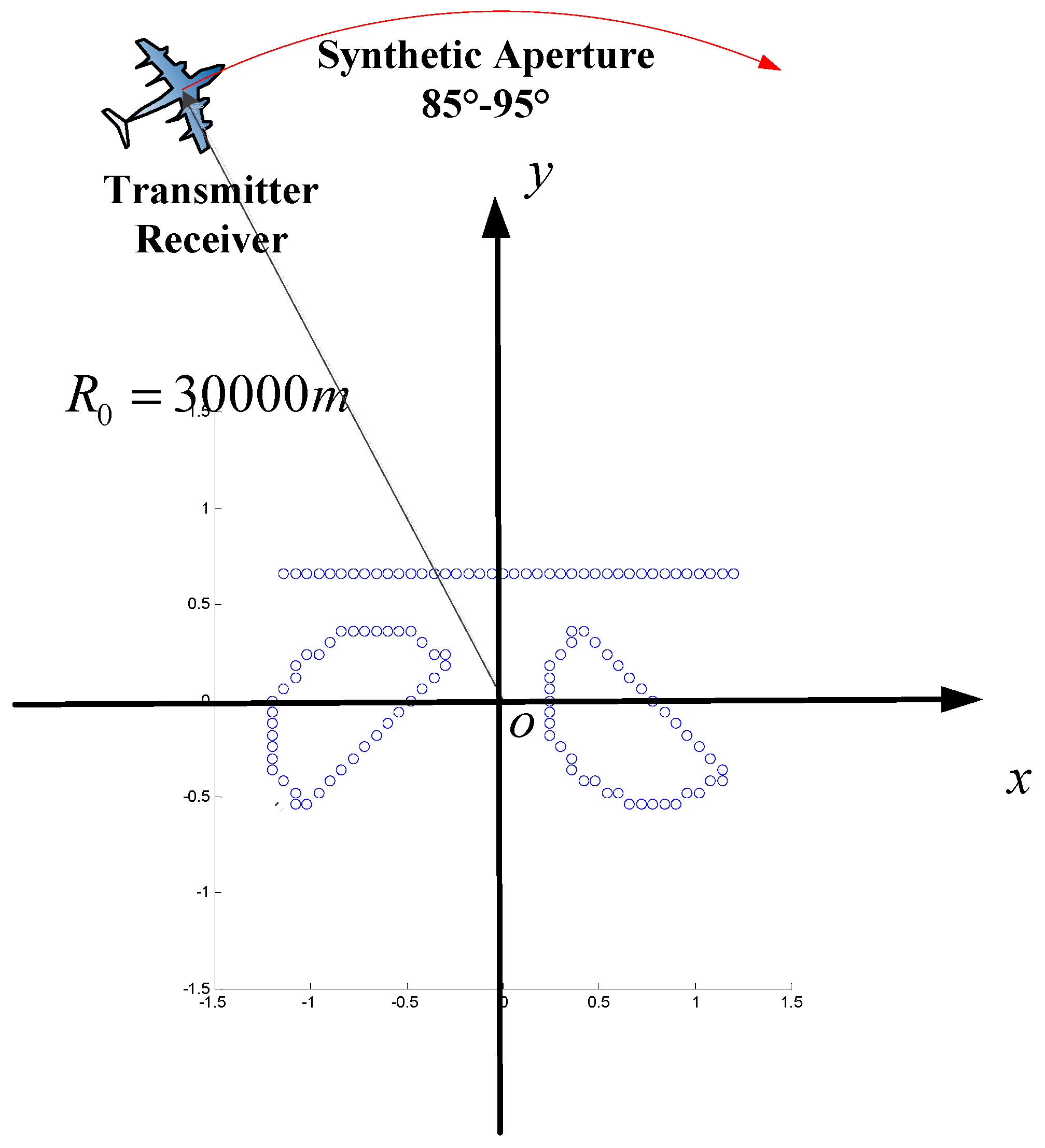
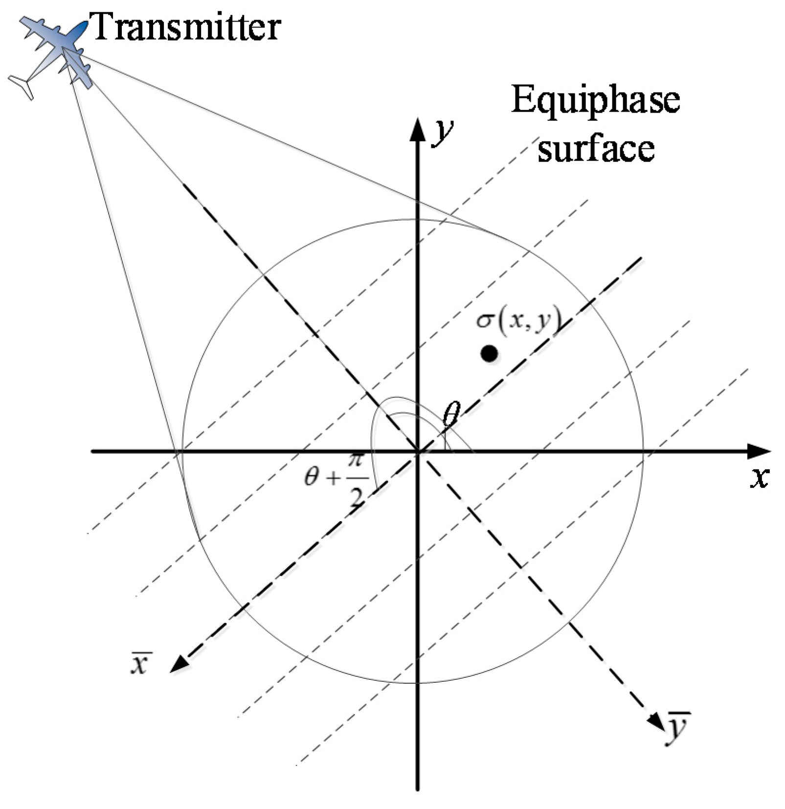
2.1. Spotlight-SAR Signal Model
2.2. Back-Projection Imaging Algorithm
- (1)
- Data acquisition: Sampling the signal received by the receiver and down-conversion.
- (2)
- Range direction compression: To accelerate the processing speed, the IFFT operation is utilized.
- (3)
- Determining the radar position and the scene location: Using the motion trajectory of the SAR platform, phase of every PRT signal is obtained to compensate the impact of wave propagation.
- (4)
- Azimuth direction compression: The second integration is computed by employing the result of Step 3.
2.3. CS-Theory Based on Single Measurement Vector
3. SAR Imaging Based on Multiple Measurement Vector Model
3.1. Structured CS Model—Multiple Measurement Vectors
3.2. Recovery Algorithms
| Algorithm 1. MMV-OMP |
| Inputs: , K, the sparsity of |
| Output: Row-sparse matrix |
| Initialization: |
| for do |
| 1 Max correlation: |
| 2 New support: |
| 3 Update Approximation: |
| 4 Update Residual: |
| end for |
| Return |
3.3. Two-Dimensional SAR Imaging Based on BP Method
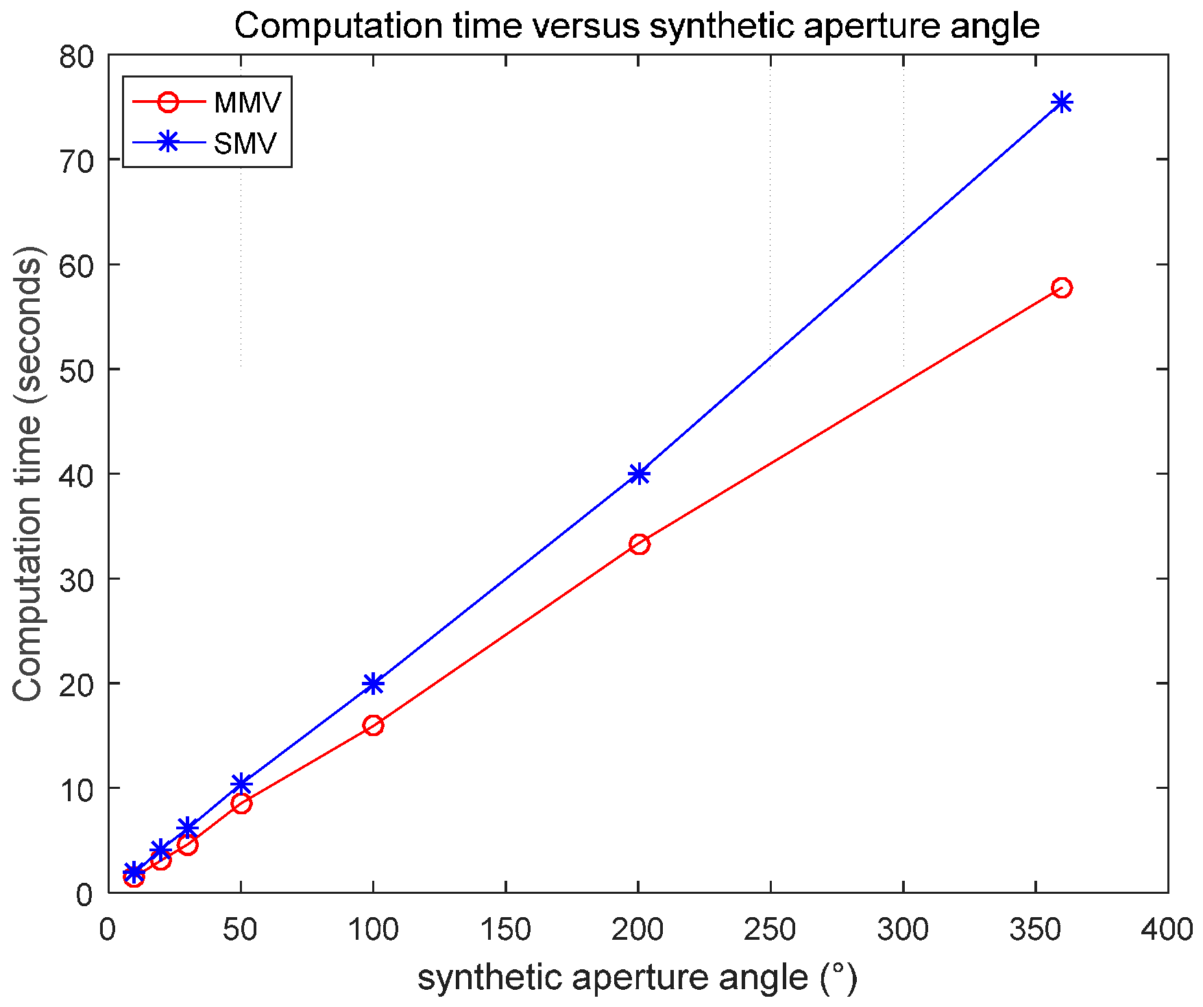
- Lower computation cost and fewer needed data: Due to the use of the MMV model, we can recovery multiple azimuth direction samples at one time with high speed and save the memory cost.
- High compatibility and high resolution: The MF-like azimuth processing to enhance the robust of the algorithm, which can fit most cases of SAR imaging. The improved CS-SAR method can take the advantage of BP and CS method, and robustly produce high-resolution images using the same amount of data.
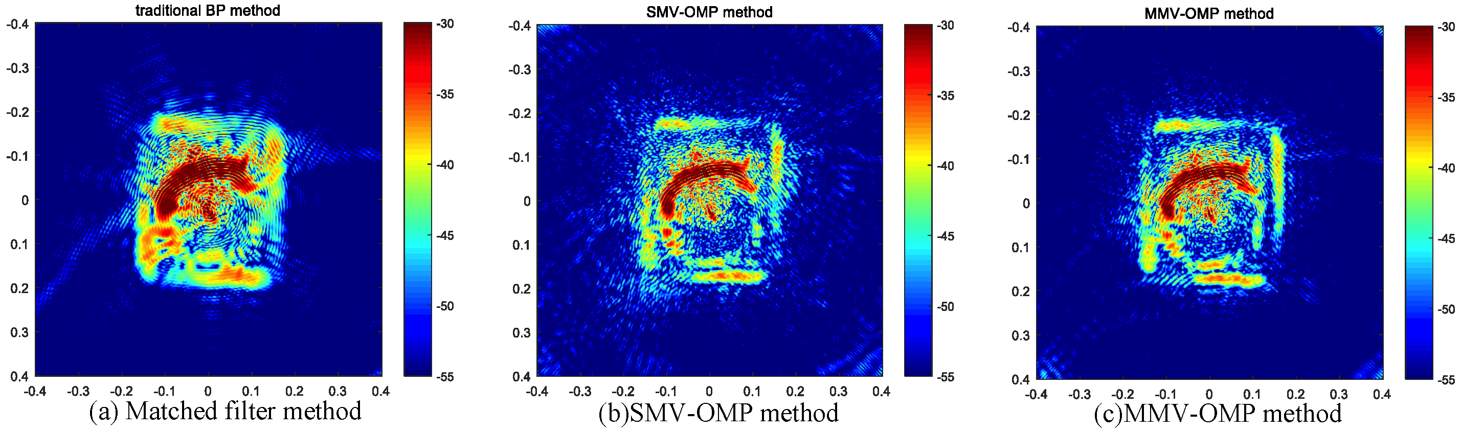
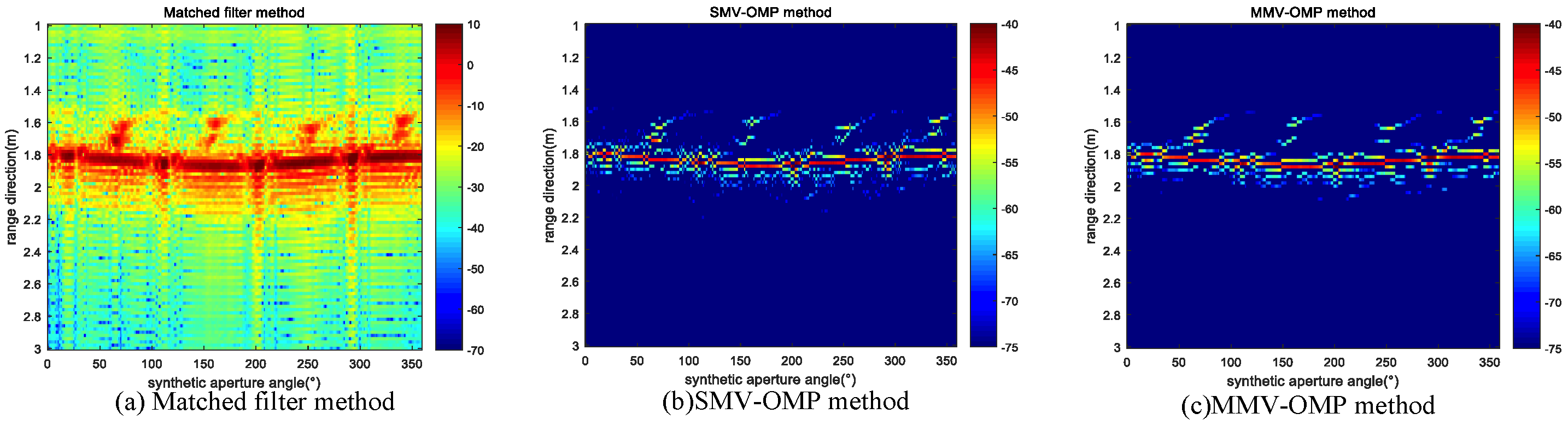
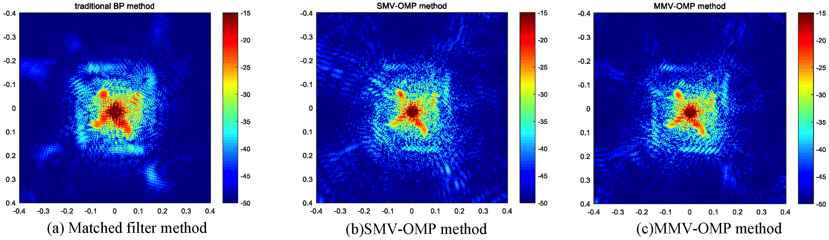
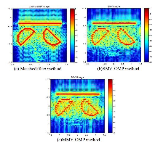
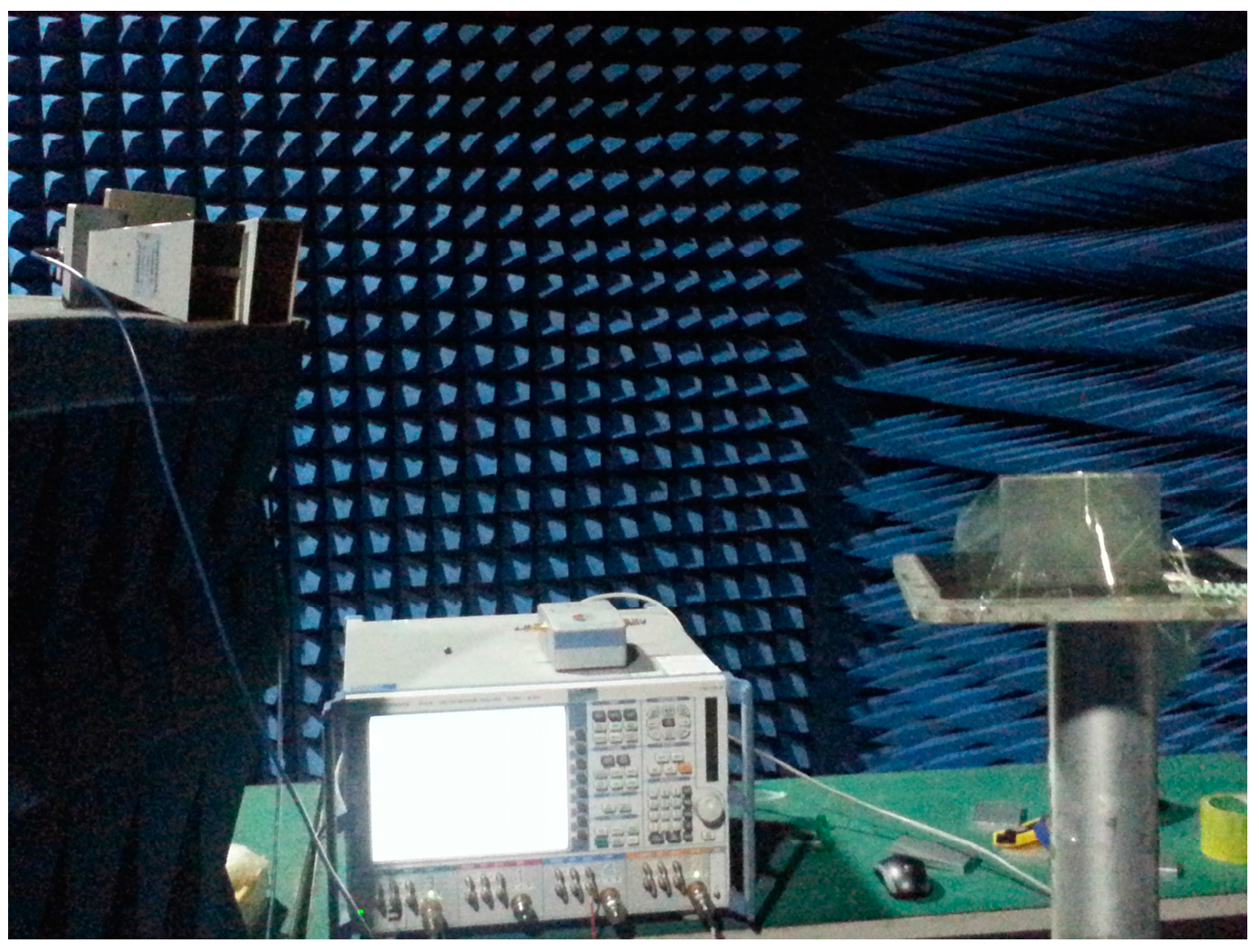
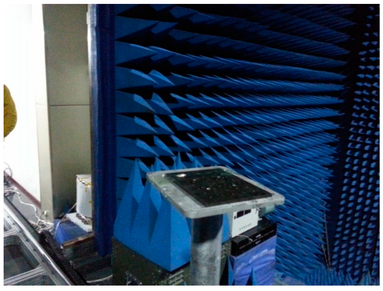
4. Simulations and Experiments
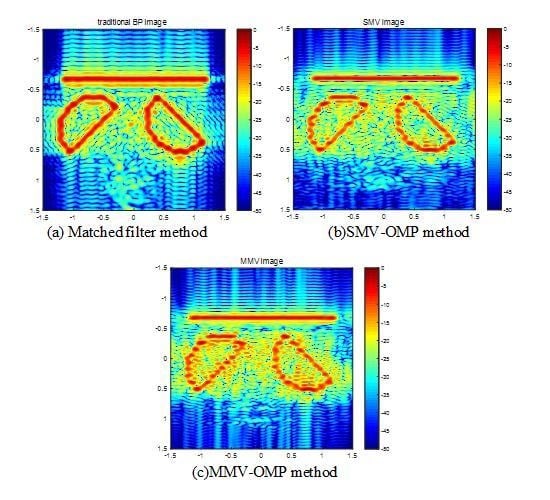
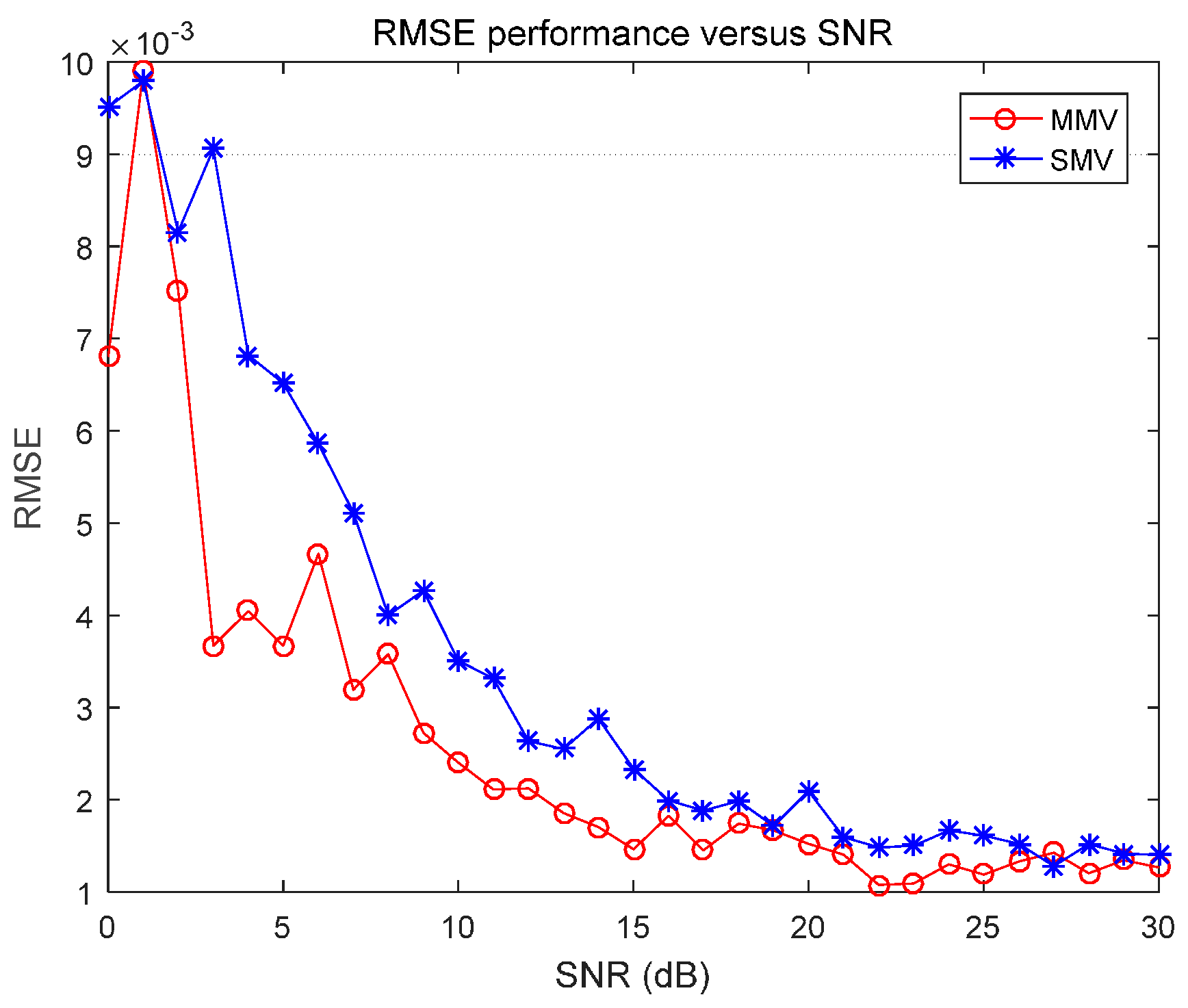
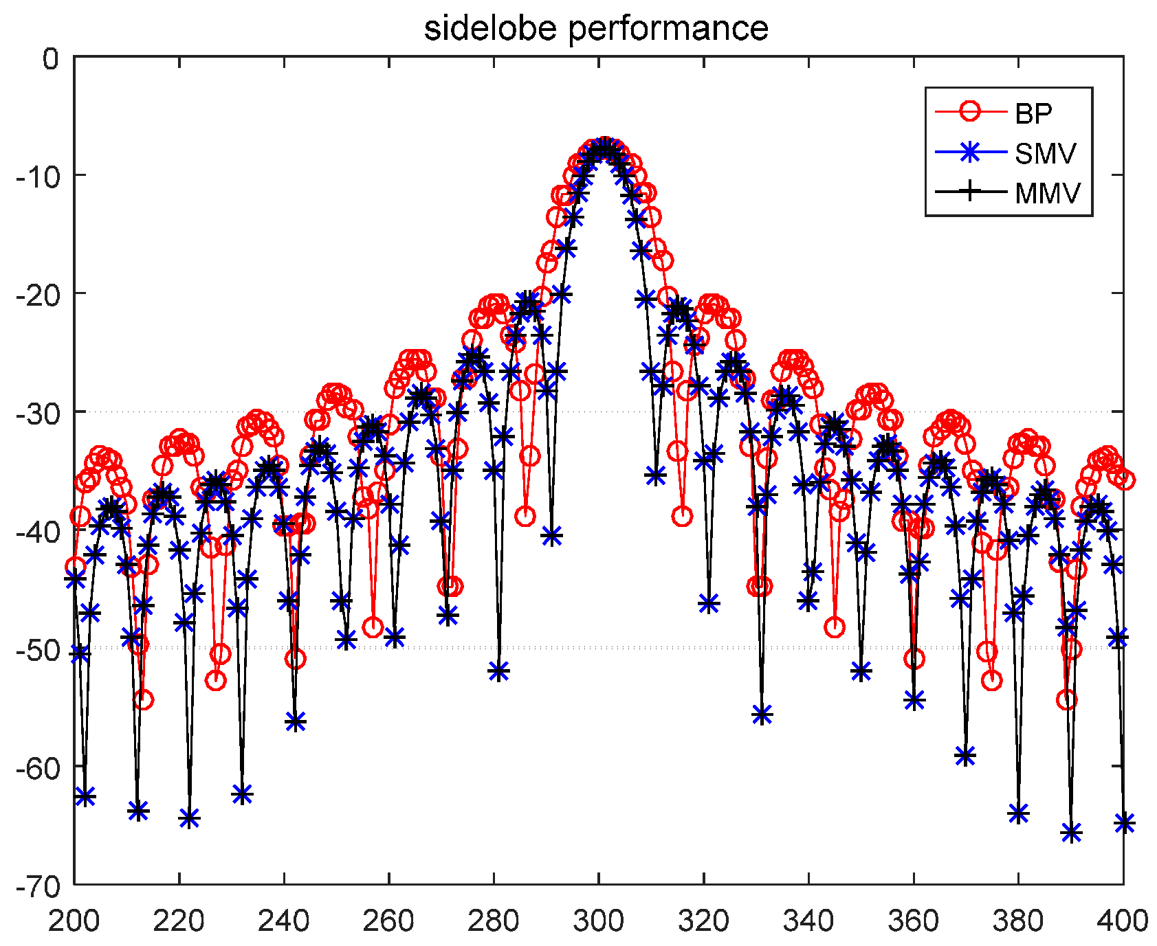
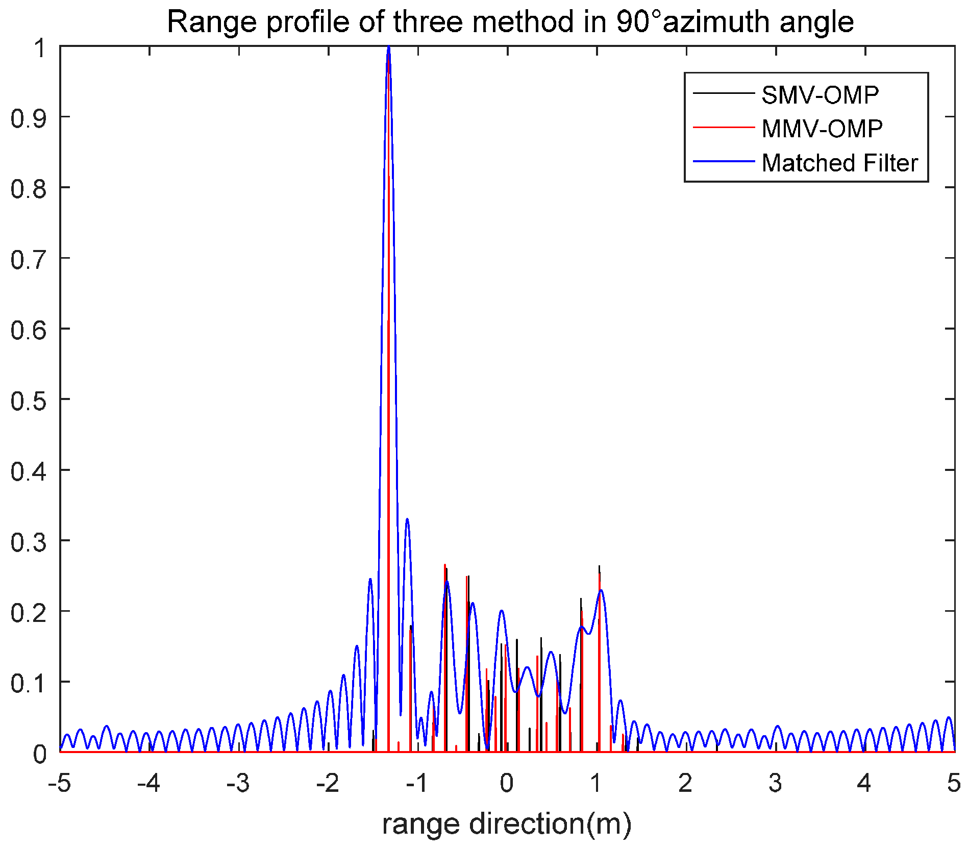
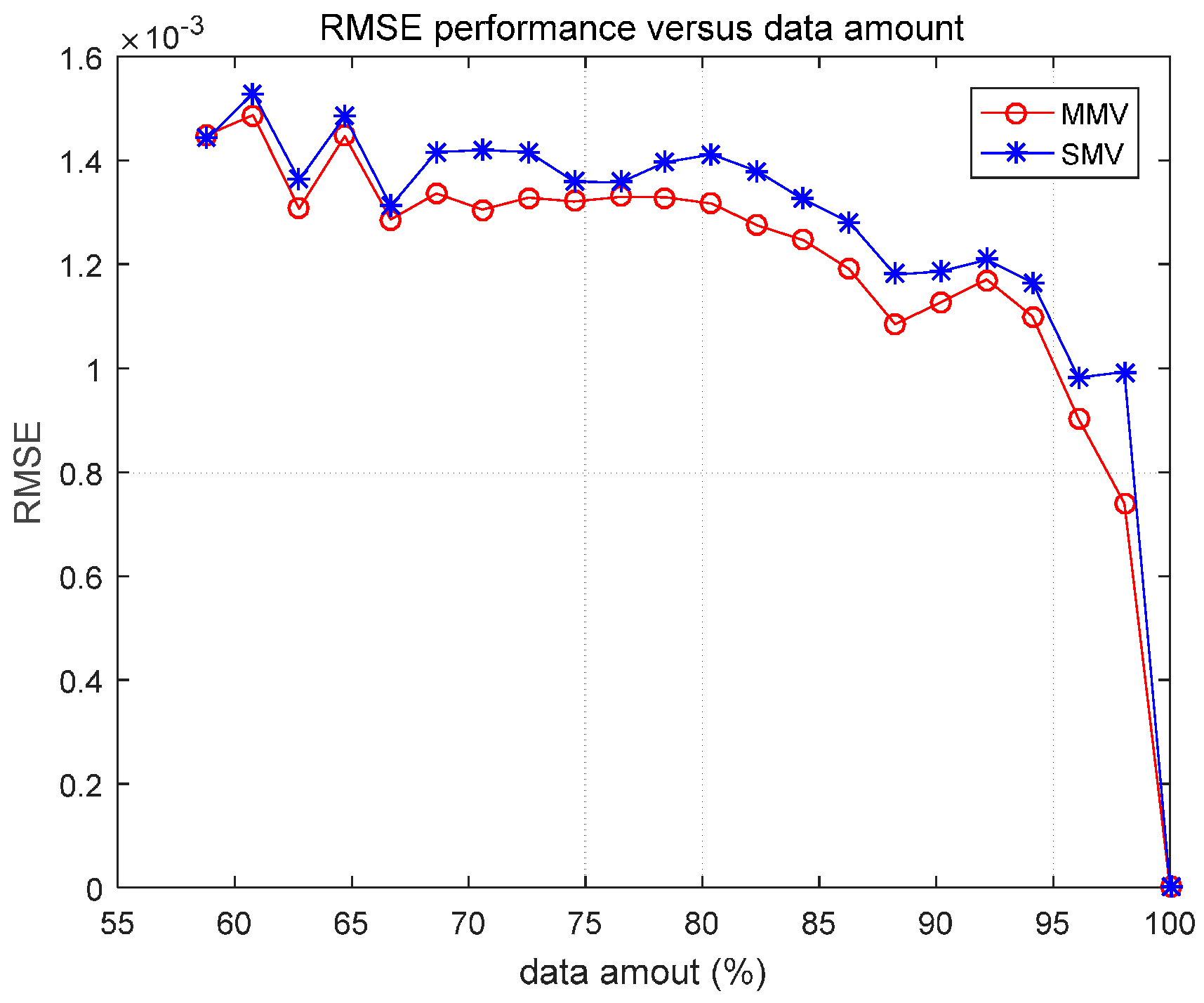
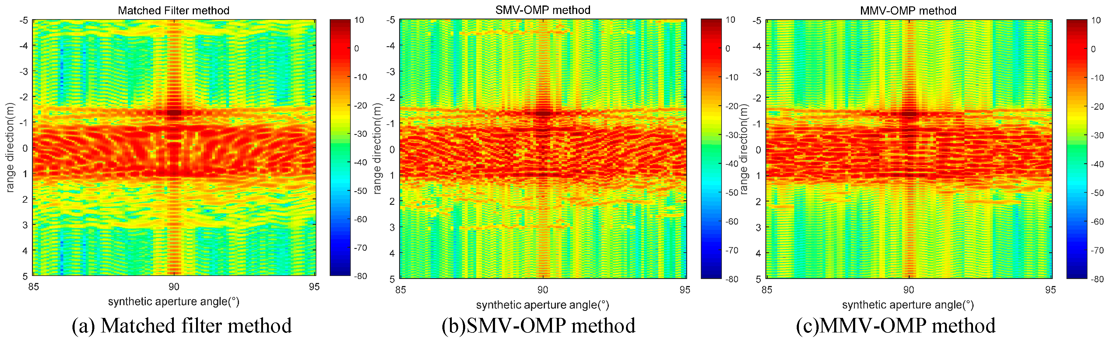
4.1. Simulations
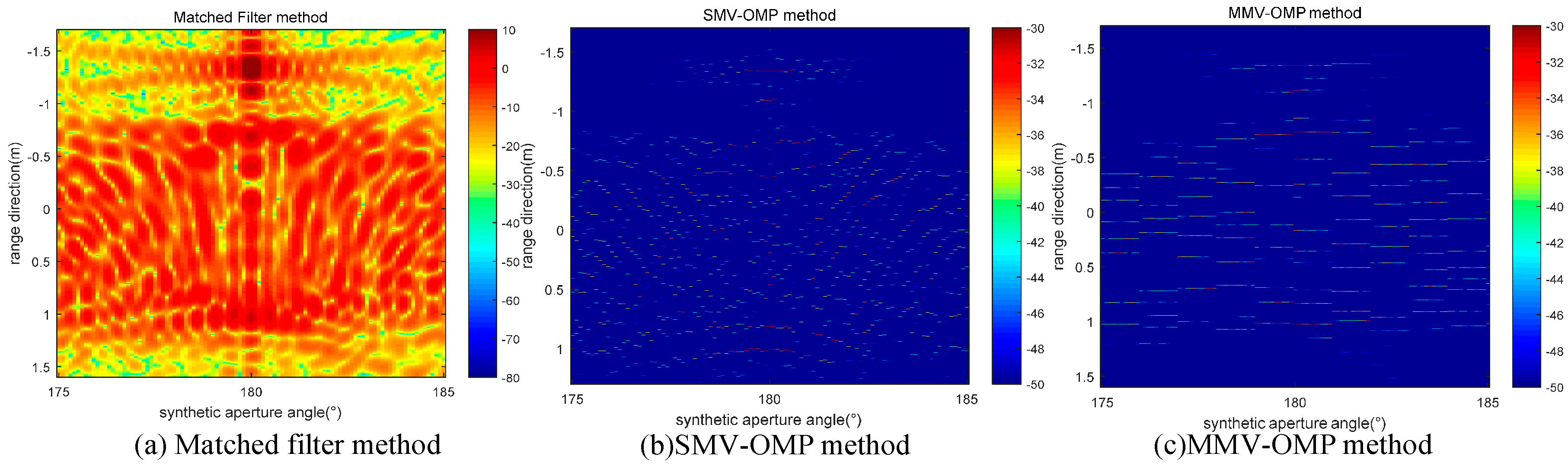
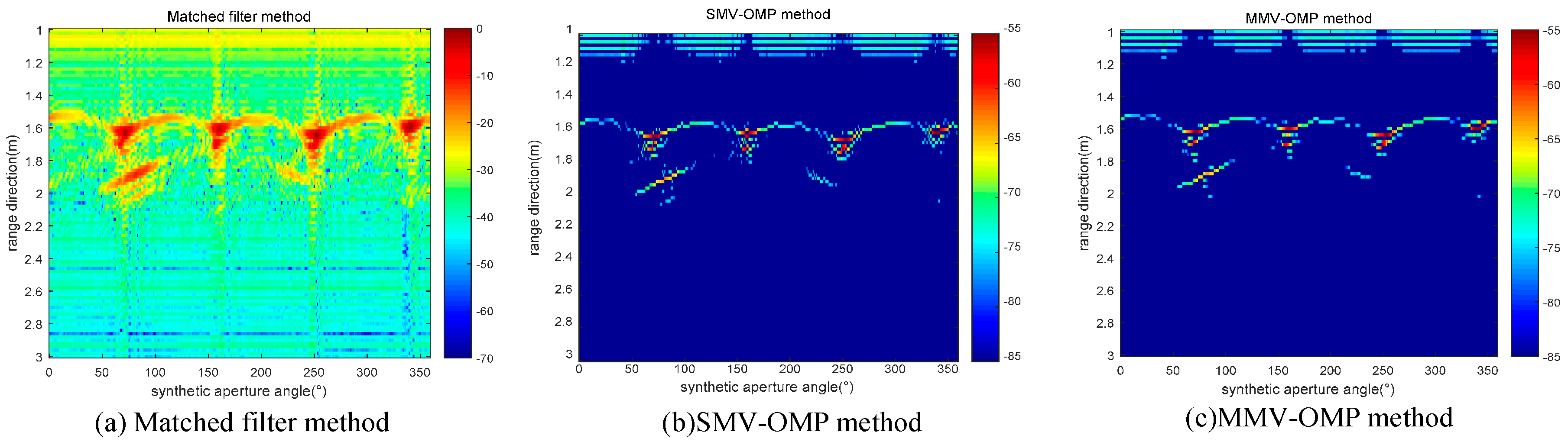
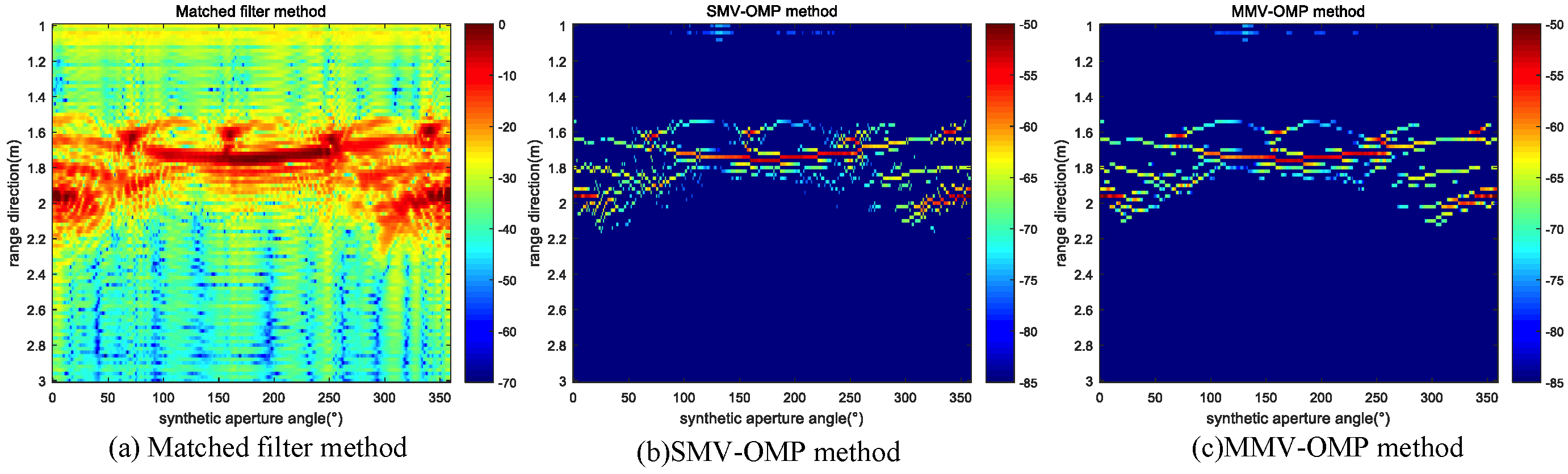
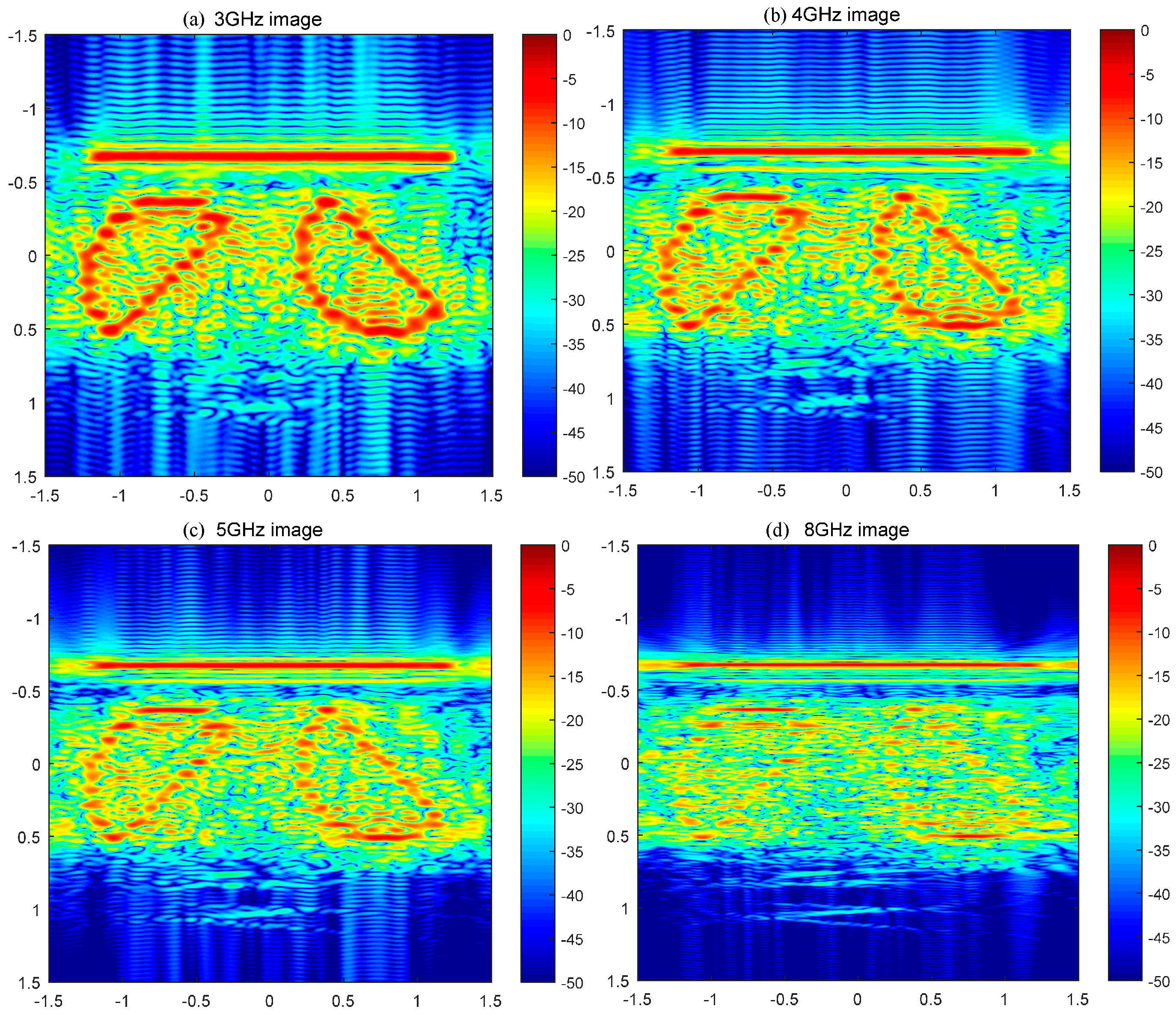
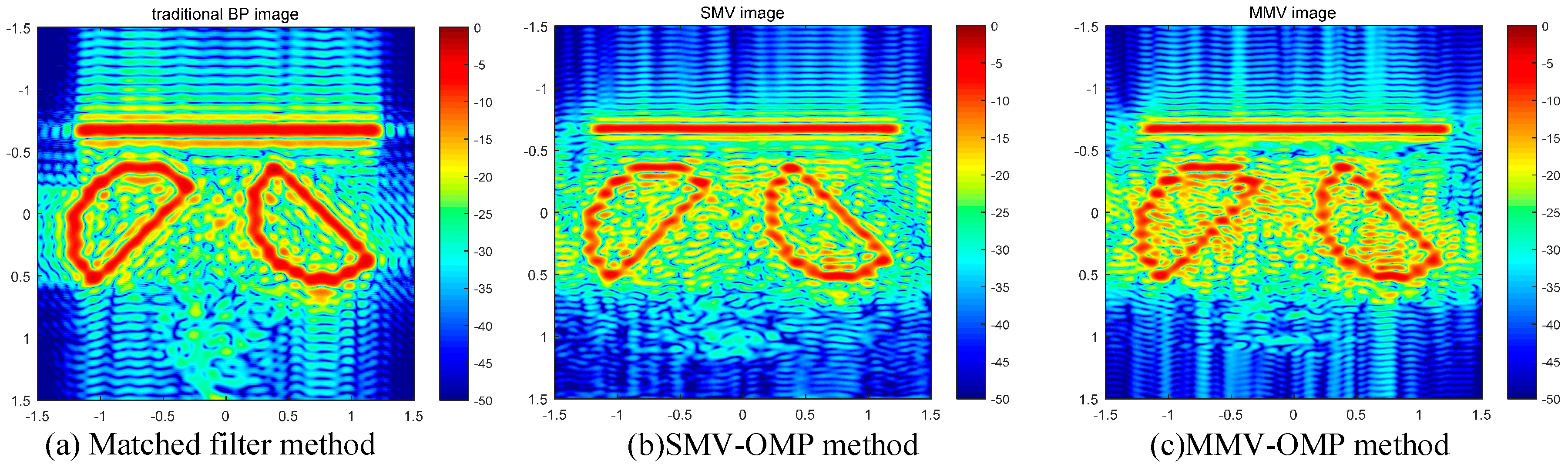
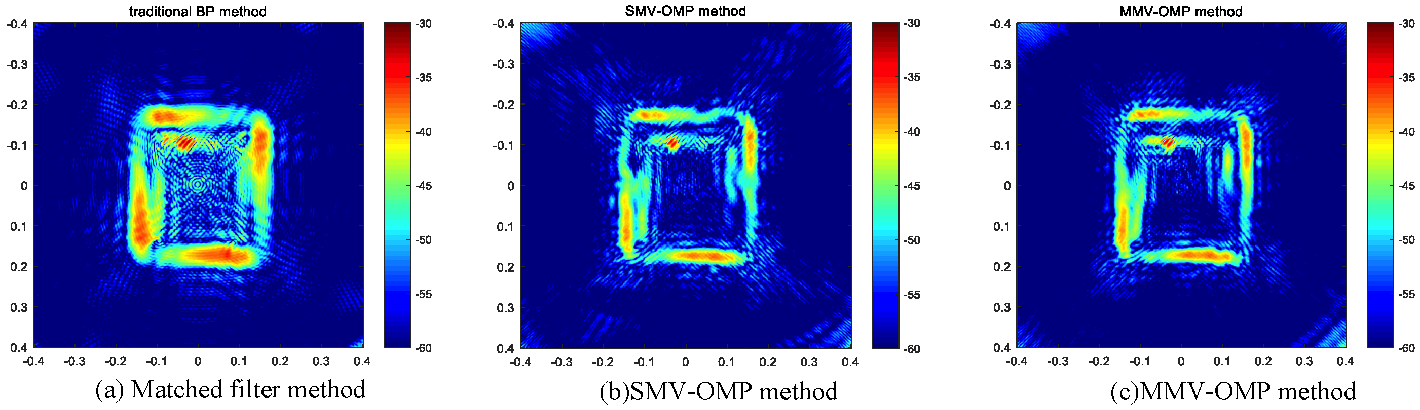
4.2. Regular Sparse Imaging and Improved Sparse Imaging Based on MMV
5. Discussion
6. Conclusions
Acknowledgments
Author Contributions
Conflicts of Interest
References
- Curlander, J.C.; McDonough, R.N. Synthetic Aperture Radar; John Wiley & Sons: New York, NY, USA, 1991. [Google Scholar]
- Yu, Z.; Wang, S.; Li, Z. An Imaging Compensation Algorithm for Spaceborne High-Resolution SAR Based on a Continuous Tangent Motion Model. Remote Sens. 2016, 8, 223. [Google Scholar] [CrossRef]
- Garzelli, A. A Review of Image Fusion Algorithms Based on the Super-Resolution Paradigm. Remote Sens. 2016, 8, 797. [Google Scholar] [CrossRef]
- Baraniuk, R.G.; Steeghs, P. Compressive radar imaging. In Proceedings of the IEEE Radar Conference, Boston, MA, USA, 17–20 April 2007; pp. 128–133.
- Patel, V.M.; Easley, G.R.; Healy, D.M., Jr.; Chellappa, R. Compressed synthetic aperture radar. IEEE J. Sel. Top. Signal Process. 2010, 4, 244–254. [Google Scholar] [CrossRef]
- Alonso, M.T.; López-Dekker, P.; Mallorquí, J.J. A novel strategy for radar imaging based on compressive sensing. IEEE Trans. Geosci. Remote Sens. 2010, 48, 4285–4295. [Google Scholar] [CrossRef]
- Zhu, X.X.; Bamler, R. Tomographic SAR inversion by L1-norm regularization—The compressive sensing approach. IEEE Trans. Geosci. Remote Sens. 2010, 48, 3839–3846. [Google Scholar] [CrossRef]
- Zhu, X.X.; Bamler, R. Super-resolution power and robustness of compressive sensing for spectral estimation with application to spaceborne tomographic SAR. IEEE Trans. Geosci. Remote Sens. 2012, 50, 247–258. [Google Scholar] [CrossRef]
- Bu, H.; Tao, R.; Bai, X.; Zhao, J. A Novel SAR Imaging Algorithm Based on Compressed Sensing. IEEE Geosci. Remote Sens. Lett. 2015, 12, 1003–1007. [Google Scholar]
- Shen, F.; Zhao, G.; Shi, G.; Dong, W.; Wang, C.; Niu, Y. Compressive SAR Imaging with Joint Sparsity and Local Similarity Exploitation. Sensors 2015, 15, 4176–4192. [Google Scholar] [CrossRef] [PubMed]
- Xiao, P.; Yu, Z.; Li, C. Compressive sensing SAR range compression with chirp scaling principle. Sci. China Inf. Sci. 2012, 55, 2292–2300. [Google Scholar] [CrossRef]
- Massa, A.; Rocca, P.; Oliveri, G. Compressive Sensing in Electromagnetics—A Review. IEEE Antennas Propag. Mag. 2015, 57, 224–238. [Google Scholar] [CrossRef]
- Phillips, J.W.; Leahy, R.M.; Mosher, J.C. MEG-based imaging of focal neuronal current sources. IEEE Trans. Med. Imaging 1997, 16, 338–348. [Google Scholar] [CrossRef] [PubMed]
- Gribonval, R. Sparse decomposition of stereo signals with matching pursuit and application to blind separation of more than two sources from a stereo mixture. In Proceedings of the IEEE International Conference Acoustics, Speech, Signal Processing (ICASSP), Minneapolis, MN, USA, 27–30 April 1993.
- Malioutov, D.; Cetin, M.; Willsky, A.S. A sparse signal reconstruction perspective for source localization with sensor arrays. IEEE Trans. Signal Process. 2005, 53, 3010–3022. [Google Scholar] [CrossRef]
- Hyder, M.M.; Mahata, K. A robust algorithm for joint-sparse recovery. IEEE Signal Process. Lett. 2009, 16, 1091–1094. [Google Scholar] [CrossRef]
- Méndez-Rial, R.; Rusu, C.; Alkhateeb, A.; González-Prelcic, N.; Heath, R.W. Channel estimation and hybrid combining for mmwave: Phase shifters or switches? In Proceedings of the Information Theory and Applications Workshop (ITA), San Diego, CA, USA, 1–6 February 2015; pp. 90–97.
- Li, Y.; Chi, Y. Off-the-grid line spectrum denoising and estimation with multiple measurement vectors. IEEE Trans. Signal Process. 2016, 64, 1257–1269. [Google Scholar] [CrossRef]
- Sharma, S.K.; Lagunas, E.; Chatzinotas, S.; Ottersten, B. Application of compressive sensing in cognitive radio communications: A survey. IEEE Commun. Surv. Tutor. 2016, 99, 1–24. [Google Scholar] [CrossRef]
- Oriot, H.; Cantalloube, H. Circular SAR imagery for urban remote sensing. In Proceedings of the 7th European Conference on Synthetic Aperture Radar (EUSAR), Friedrichshafen, Germany, 2–5 June 2008; pp. 1–4.
- Li, B.; Liu, F.; Zhou, C.; Lv, Y.; Hu, J. Fast compressed sensing SAR imaging using stepped frequency waveform. In Proceedings of the 2016 IEEE International Conference on Microwave and Millimeter Wave Technology (ICMMT), Beijing, China, 5–8 June 2016; pp. 521–523.
- Chen, J.; Zeng, T.; Long, T. A novel high-resolution stepped frequency SAR signal processing method. In Proceedings of the IET International Radar Conference, Guilin, China, 20–22 April 2009; pp. 1–4.
- Yang, J.; Huang, X.; Jin, T.; Thompson, J.; Zhou, Z. Synthetic aperture radar imaging using stepped frequency waveform. IEEE Trans. Geosci. Remote Sens. 2012, 50, 2026–2036. [Google Scholar] [CrossRef]
- Shkvarko, Y.V.; Yañez, J.I.; Amao, J.A.; del Campo, G.D.M. Radar/SAR Image Resolution Enhancement via Unifying Descriptive Experiment Design Regularization and Wavelet-Domain Processing. IEEE Geosci. Remote Sens. Lett. 2016, 13, 152–156. [Google Scholar] [CrossRef]
- Duarte, M.F.; Eldar, Y.C. Structured compressed sensing: From theory to applications. IEEE Trans. Signal Process. 2011, 59, 4053–4085. [Google Scholar] [CrossRef]
- Rauhut, H. Compressive Sensing and Structured Random Matrices. In Theoretical Foundations and Numerical Methods for Sparse Recovery; Fornasier, M., Ed.; deGruyter: Goetingen, Germany, 2010; Volume 9, pp. 1–92. [Google Scholar]
- Tropp, J.A.; Laska, J.N.; Duarte, M.F.; Romberg, J.K.; Baraniuk, R.G. Beyond Nyquist: Efficient Sampling of Sparse Bandlimited Signals. IEEE Trans. Inf. Theory 2010, 56, 520–544. [Google Scholar] [CrossRef]
- Baron, D.; Wakin, M.B.; Duarte, M.F.; Sarvotham, S.; Baraniuk, R.G. Distributed compressed sensing. IEEE Trans. Inf. Theory 2006, 52, 5406–5425. [Google Scholar]
- Davies, M.E.; Eldar, Y.C. Rank awareness in joint sparse recovery. IEEE Trans. Inf. Theory 2012, 58, 1135–1146. [Google Scholar] [CrossRef]
- Mishali, M.; Eldar, Y.C. Reduce and boost: Recovering arbitrary sets of jointly sparse vectors. IEEE Trans. Signal Process. 2008, 56, 4692–4702. [Google Scholar] [CrossRef]
- Leviatan, D.; Temlyakov, V.N. Simultaneous approximation by greedy algorithms. Adv. Comput. Math. 2006, 25, 73–90. [Google Scholar] [CrossRef]
- Tropp, J.A.; Gilbert, A.C.; Strauss, M.J. Algorithms for simultaneous sparse approximation. Part I: Greedy pursuit. Signal Process. 2006, 86, 572–588. [Google Scholar] [CrossRef]
- Blanchard, J.D.; Cermak, M.; Hanle, D.; Jing, Y. Greedy Algorithms for Joint Sparse Recovery. IEEE Trans. Signal Process. 2014, 62, 1694–1704. [Google Scholar] [CrossRef]
- Gorodnitsky, I.F.; Rao, B.D. Sparse signal reconstruction from limited data using FOCUSS: A re-weighted minimum norm algorithm. IEEE Trans. Signal Process. 1997, 45, 600–616. [Google Scholar] [CrossRef]
- Chen, S.S.; Donoho, D.L.; Saunders, M.A. Atomic decomposition by basis pursuit. SIAM J. Sci. Comput. 1998, 20, 33–61. [Google Scholar] [CrossRef]
- Song, S.; Xu, B.; Yang, J. SAR Target Recognition via Supervised Discriminative Dictionary Learning and Sparse Representation of the SAR-HOG Feature. Remote Sens. 2016, 8, 683. [Google Scholar] [CrossRef]
- Pati, Y.C.; Rezaiifar, R.; Krishnaprasad, P. Orthogonal matching pursuit: Recursive function approximation with applications to wavelet decomposition. In Proceedings of the Twenty-Seventh Asilomar Conference on Signals, Systems and Computers, Pacufic Grove, CA, USA, 1–3 November 1993; pp. 40–44.
- Gribonval, R.; Rauhut, H.; Schnass, K.; Vandergheynst, P. Atoms of all channels, unite! Average case analysis of multi-channel sparse recovery using greedy algorithms. J. Fourier Anal. Appl. 2008, 14, 655–687. [Google Scholar] [CrossRef]


| Carrier Frequency | 10 GHz |
| Bandwidth | 2 GHz |
| Frequency interval | 40 MHz |
| Angle Range | 85°–95° |
| Angle interval | 0.1° |
| Initial Distance | 30,000 m |
| BP | SMV | MMV | |
|---|---|---|---|
| PSLR (dB) | 13.2474 | 13.3782 | 13.3782 |
| ISLR (dB) | 9.8874 | 9.9592 | 9.9592 |
| main lobe width (m) | 0.09 | 0.05 | 0.05 |
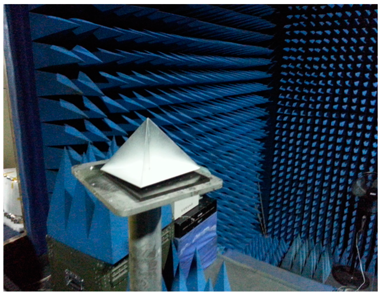
| Carrier Frequency | 15 GHz |
| Bandwidth | 6 GHz |
| Frequency interval | 15 MHz |
| Angle Range | 1° ~ 360° |
| Angle interval | 1° |
| Initial Distance | 0.91 m |
| Antenna Gain | 10 dB |
| Antenna frequency | 12–28 GHz |
| Antenna beamwidth | 10° |
© 2017 by the authors. Licensee MDPI, Basel, Switzerland. This article is an open access article distributed under the terms and conditions of the Creative Commons Attribution (CC BY) license ( http://creativecommons.org/licenses/by/4.0/).
Share and Cite
Ao, D.; Wang, R.; Hu, C.; Li, Y. A Sparse SAR Imaging Method Based on Multiple Measurement Vectors Model. Remote Sens. 2017, 9, 297. https://doi.org/10.3390/rs9030297
Ao D, Wang R, Hu C, Li Y. A Sparse SAR Imaging Method Based on Multiple Measurement Vectors Model. Remote Sensing. 2017; 9(3):297. https://doi.org/10.3390/rs9030297
Chicago/Turabian StyleAo, Dongyang, Rui Wang, Cheng Hu, and Yuanhao Li. 2017. "A Sparse SAR Imaging Method Based on Multiple Measurement Vectors Model" Remote Sensing 9, no. 3: 297. https://doi.org/10.3390/rs9030297
APA StyleAo, D., Wang, R., Hu, C., & Li, Y. (2017). A Sparse SAR Imaging Method Based on Multiple Measurement Vectors Model. Remote Sensing, 9(3), 297. https://doi.org/10.3390/rs9030297