Article

Mapping of Vegetation Using Multi-Temporal Downscaled Satellite Images of a Reclaimed Area in Saemangeum, Republic of Korea

1
Department of Landscape Architecture, Chonbuk National University, 567 Baekje-daero, Jeonju-si 54896, Korea
2
Earth Observation Research Team, Korea Aerospace Research Institute, 169-84, Gwahak-ro, Yuseong-Gu, Daejeon 34133, Korea
3
Dongyeong Forest, Keimyung University, 1095 Dalgubeol-daero, Dalseo-gu, Daegu Metropolitan City 42601, Korea
4
Department of Geographic Information Systems Engineering, Namseoul University, 91 Daehak-ro Seonghwan-eup Sebuk-gu, Cheonan-si 31020, Korea
*
Author to whom correspondence should be addressed.
Remote Sens. 2017, 9(3), 272; https://doi.org/10.3390/rs9030272
Submission received: 12 January 2017 / Revised: 3 March 2017 / Accepted: 12 March 2017 / Published: 15 March 2017

Abstract

:
The aim of this study is to adapt and evaluate the effectiveness of a multi-temporal downscaled images technique for classifying the typical vegetation types of a reclaimed area. The areas reclaimed from estuarine tidal flats show high spatial heterogeneity in soil salinity conditions. There are three typical vegetation types for which the distribution is restricted by the soil conditions. A halophyte-dominated vegetation is located in a high saline area, grass vegetation is found in a mid- or low saline area, and reed/small-reed vegetation is situated in a low saline area. Multi-temporal satellite images were used to classify the vegetation types. Landsat images were downscaled to take into account spatial heterogeneity using cokriging. A random forest classifier was used for the classification, with downscaled Landsat and RapidEye images. Classification with RapidEye images alone demonstrated a lower level of accuracy than when combined with multi-temporal downscaled images. The results demonstrate the usefulness of a downscaling technique for mapping. This approach can provide a framework which is able to maintain low costs whilst producing richer images for the monitoring of a large and heterogeneous ecosystem.

Graphical Abstract

1. Introduction

The accomplishment of many reclamation projects has changed tidal flats into agricultural areas on the West Sea coast of the Korean Peninsula. The Saemangeum is one of the largest reclamation projects in the Republic of Korea. The reclaimed areas have typical ecological characteristics. The soil salinity of the land is usually high, which leads to harsh conditions for plants, restricting the colonization of new plants and the development of vegetation. Until the soil salinity reaches a normal level, it is a strong driving force in regulating the distribution of vegetation communities within the area. The soil salinity in the area is continuously changing and heterogeneous [1,2], and as a result, it shapes the unique and dynamic characteristics of the ecosystems.
To understand the development and change of these vegetation communities, it is critical to determine the distribution of vegetation types that have different resistances to salinity. Studies of vegetation in reclaimed areas are relatively rare [1,2,3,4,5] in Korea compared to studies in salt marshes [6,7,8,9,10]. The studies have primarily focused on the relationship between the soil conditions and physiological traits of plants in reclaimed areas. Lee et al. [4] surveyed four tidal reclamation project areas and concluded that the distribution of plants was strongly restricted by the soil salinity. The clear relationship between the soil salinity and the distribution of vegetation was also found in the Saemangeum area [1,3]. Kim et al. [3] classified the vegetation types of the Saemangeum area as: (1) halophyte vegetation located in a high saline area (mean electrical conductivity (EC): 14 dSm-1), dominated by Salicornia europaea, Suaeda asparagoides, and S. japonica; (2) mixed halophyte vegetation located in mid saline areas (mean EC: 6.7 dSm-1), dominated by Phragmites communis, Puccinellia nipponica, and Carex pumila; and (3) low-saline vegetation located in low saline areas (mean EC: 3.0 dSm-1), dominated by diverse plants, including Aster subulatus, A. tripolium, and Echinochloa spp. Despite the physiological relationships, there is a limited understanding of the ecosystem conditions in a spatial context because these studies were usually conducted at experimental sites [1,2,3,5].
Remote sensing is an effective method for estimating or mapping target quantities in a large area. It is cost-effective, rapid, and able to cover a large area. Remote sensing has also been extensively used to estimate vegetation in salt marshes [6,7,11,12,13,14,15,16,17], but there is little research on using remotely sensed data for reclaimed areas [18]. In salt marsh studies, many researchers have tackled classifying halophyte plant and/or vegetation types that share many common characteristics of vegetation in an area reclaimed from estuarine tidal flats. Some studies have focused on (multi-temporal) spectral differences [6,7,11,16,17], whilst others have concentrated on classification methods such as Neural Networks Classification [12] or the random forest method [19].
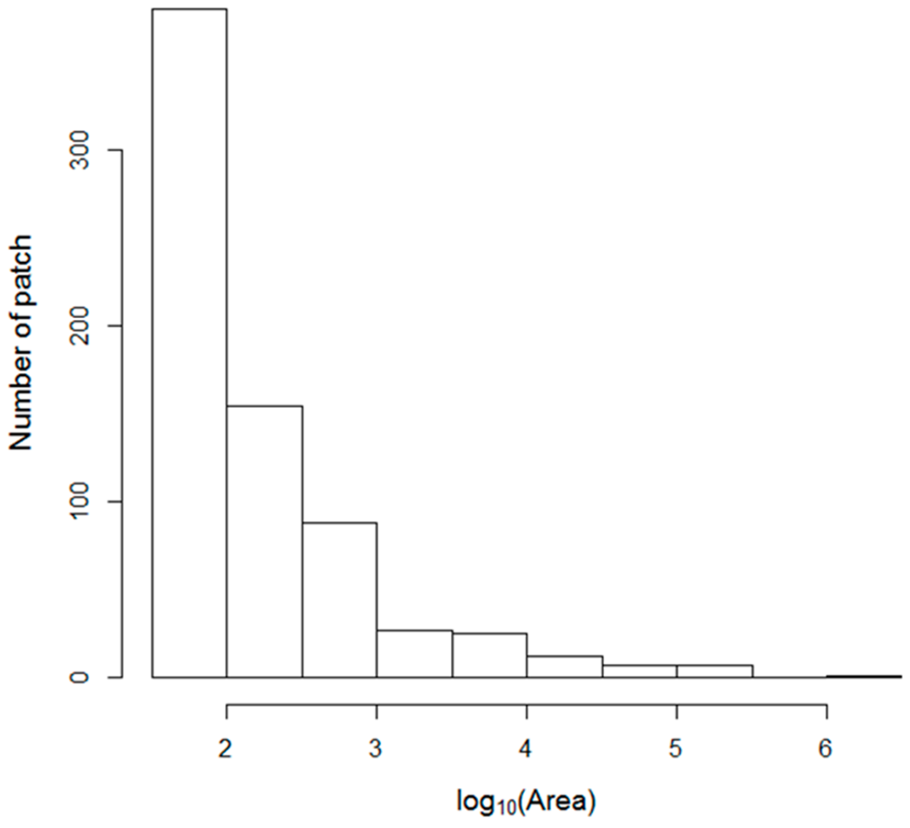
For the application of remote sensing techniques to be effective, remotely sensed data should have a strong connection to the target quantity or characteristics, in addition to the proper resolution, in order to take into account spatial variability. Vegetation in the Saemangeum is dominated by grass/herbaceous plants, and the biomass is low. The vegetation types show similar spectral responses, which makes it difficult to classify the types using spectral characteristics alone. Additionally, the vegetation patches are diverse in terms of size and shape. The patch sizes vary from several m2 to thousands of m2, and the shapes are irregular. To take into account spatial heterogeneity, it is important to select the proper resolution of the image.
It is well known that the phenological traits of vegetation can be used to improve the accuracy of vegetation or plant species mapping [11,20,21,22]. The plants in the study area primarily appear after the rainy season (mid-June to mid-July), due to the dry soil conditions in the spring. The biomass reaches a maximum in late-August to mid-September. Gilmore et al. [11] found that information on phenological variability in the growing season was useful for distinguishing dominant marsh plant species. However, it is difficult to obtain multi-temporal images with a high resolution during the short growing season. If images with short revisit frequencies and coarse resolutions can be downscaled (i.e., increased in spatial resolution), the utility of the images can be effectively increased.
The downscaling of imagery has gained attention in recent years, and many approaches have been developed (see Atkinson [23]). Among them, the use of cokriging for image sharpening provides several advantages. Cokriging has a well-established theoretical model and uses semivariograms and cross-variograms of two or more images of different resolutions [24,25,26]. Because cokriging is a generic tool, it is possible to include diverse types of data, such as topographic maps, thematic maps, or experimental data. Additionally, the downscaling cokriging method has demonstrated a lower error (mean error and mean squared error) than the method of using a high pass filter [24].
The objective of this study was to propose a modified approach to map vegetation in a reclaimed area using multi-temporal downscaled images. This study used cokriging methods to downscale Landsat imagery to the resolution of a RapidEye image. This study provides an effective method for creating an accurate vegetation map, which is essential for monitoring and managing the ecosystem of the reclaimed Saemangeum area.

2. Materials and Methods

2.1. Study Area

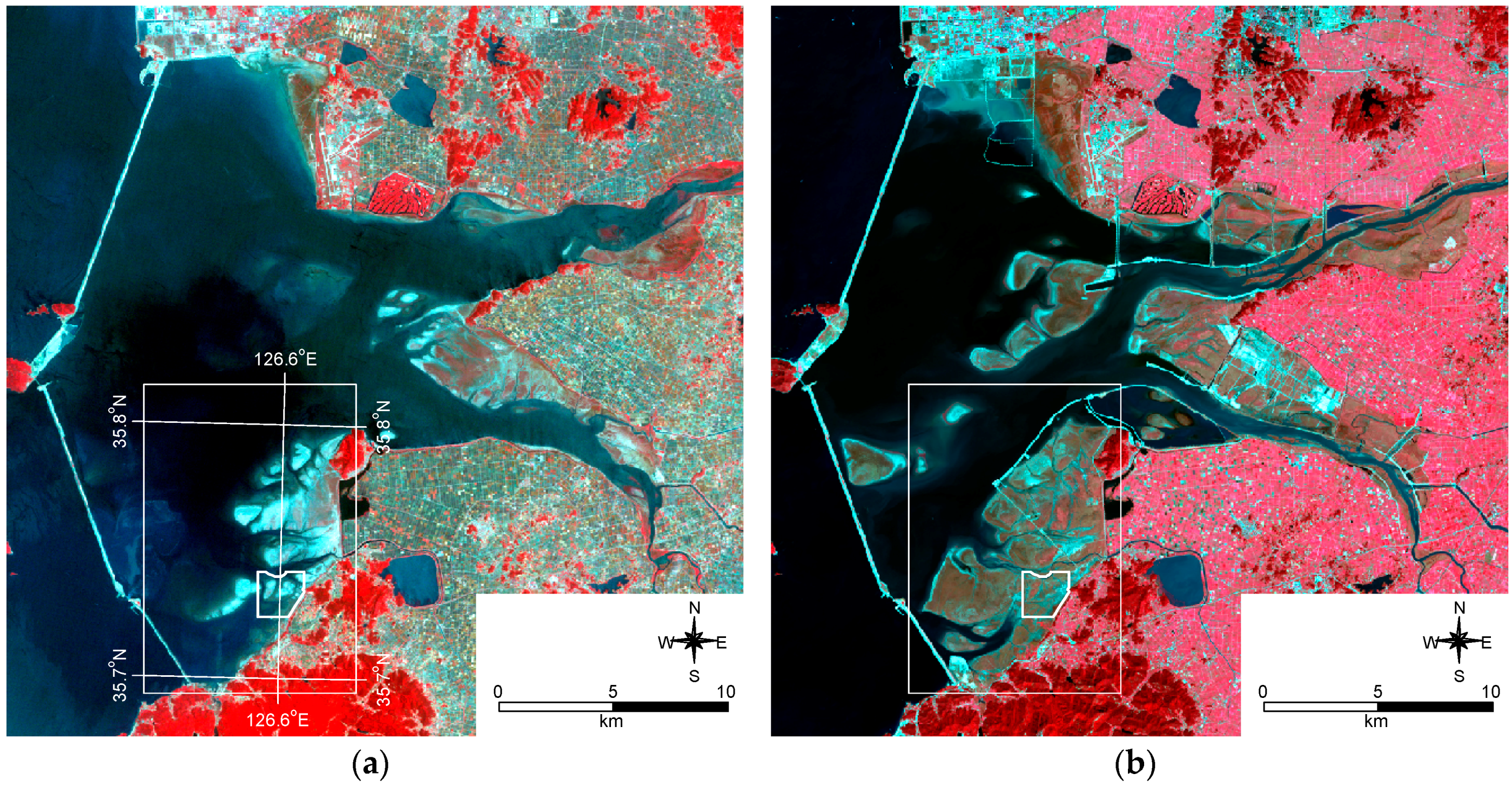
The Saemangeum is a reclaimed area that was created by the construction of a sea dike (33 km) across an estuarine tidal flat on the West Sea coast of South Korea (completed in April 2010). The dike encloses a total area of 401 km 2 (281 km 2 of land and 120 km 2 of fresh water reservoir). Although there are many reclaimed areas in Korea, the Saemangeum is unique because of its large scale and relatively long development period. These conditions allow large areas to remain under natural conditions, with very limited anthropogenic disturbance to the vegetation. It is worth noting that the soil is not imported from outside of the reclamation area, due to its large scale. The reclaimed land was created by lowering the water elevation level (EL). Since the end of 2010, the EL has been maintained at about −1.5 m (below sea level, Figure 1). At the EL, a large area of estuarine tidal flat (ca. 180 km 2 ) became land [27], while some portions of the area remained natural. The study area was selected, based on the criteria of: (1) minimal anthropogenic disturbance; and (2) heterogeneity and typical vegetation type of the reclamation area (Figure 1).

2.2. Collecting Field Data

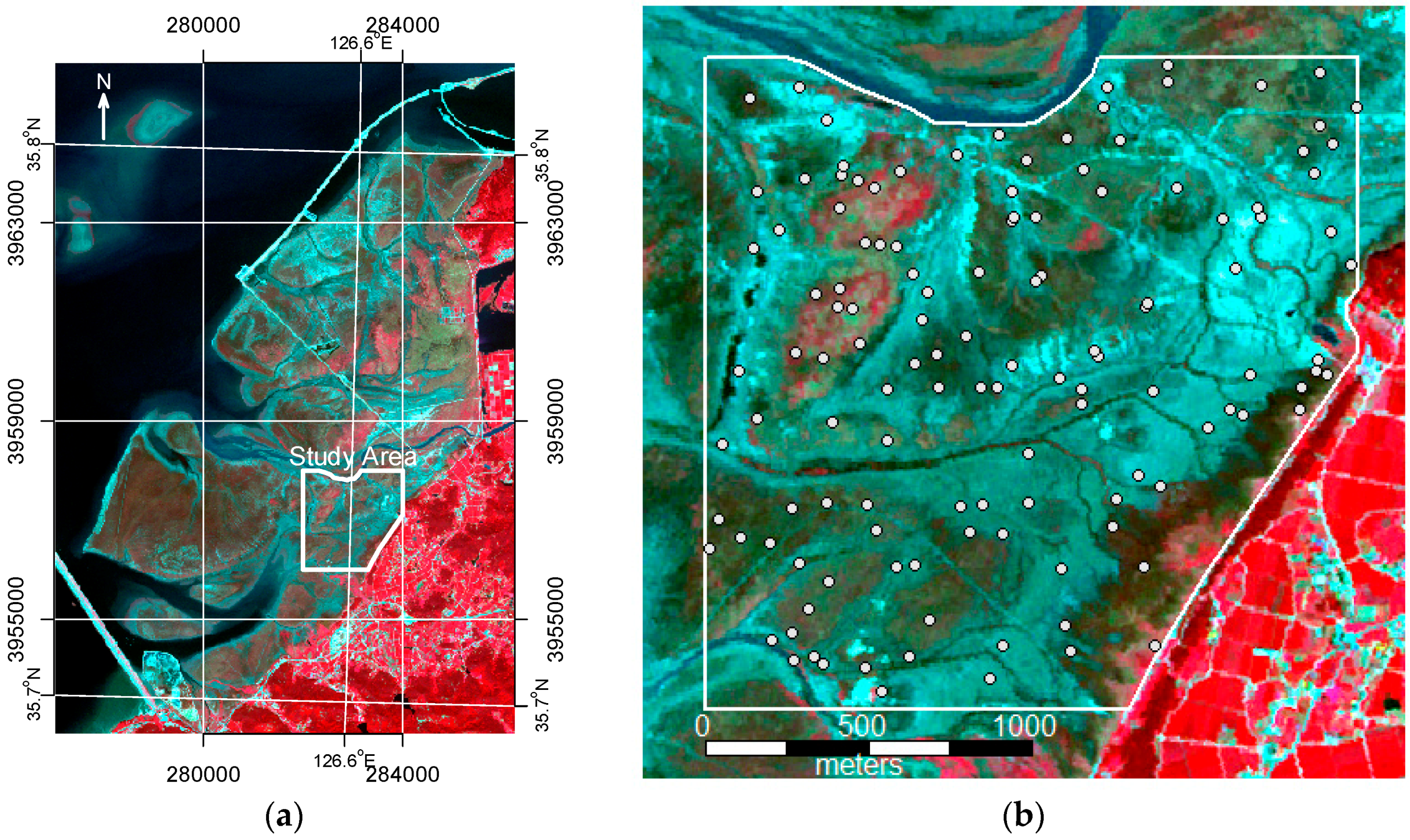
The study area was approximately 3.5 km2. A total of 127 sample plots (each plot: 5 m × 5   m ) were selected by simple random sampling (
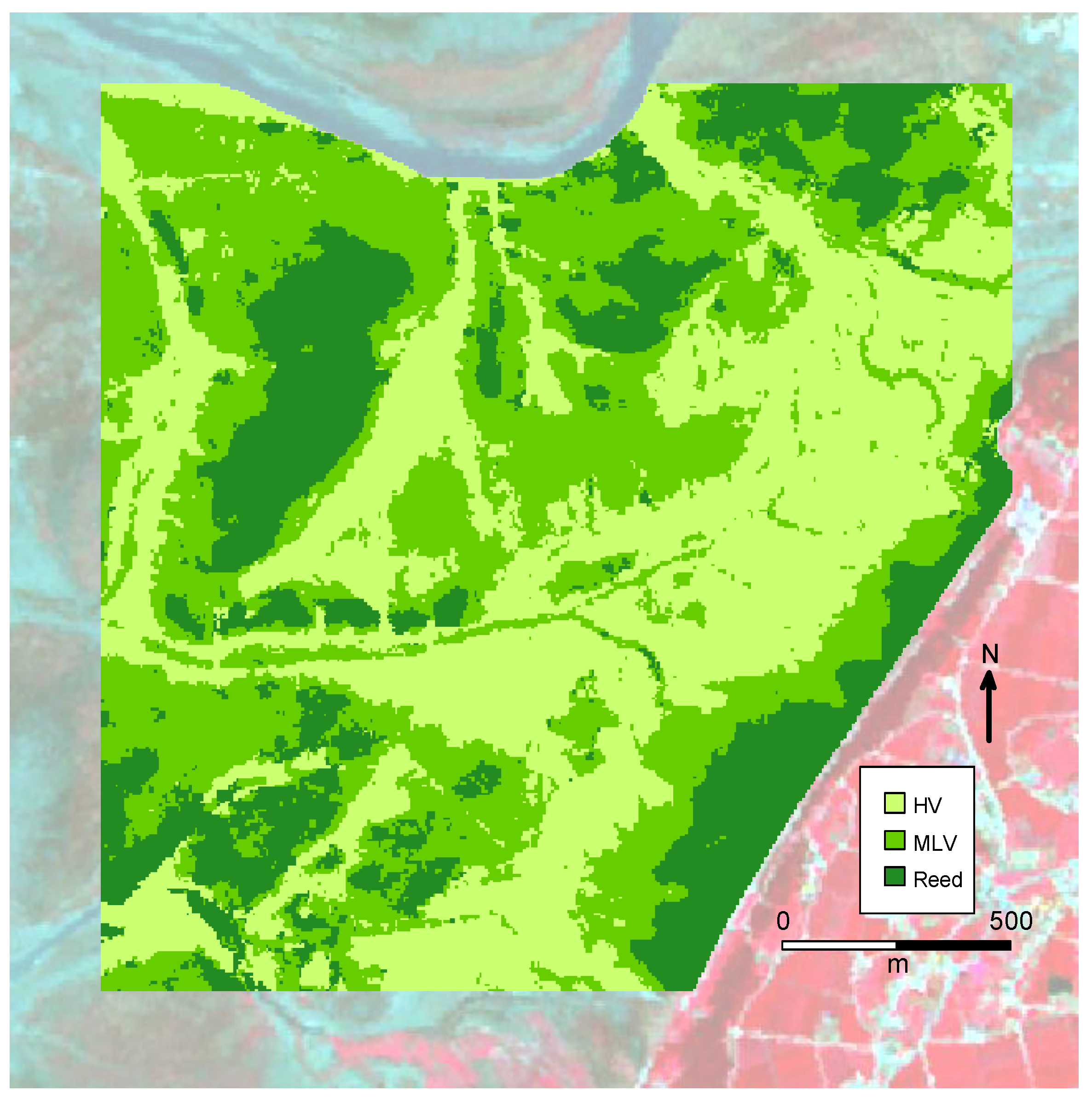
Figure 2) within the study area. A field survey was conducted in September 2014. We recorded the coverage of each species and dominant vegetation type within 25 m
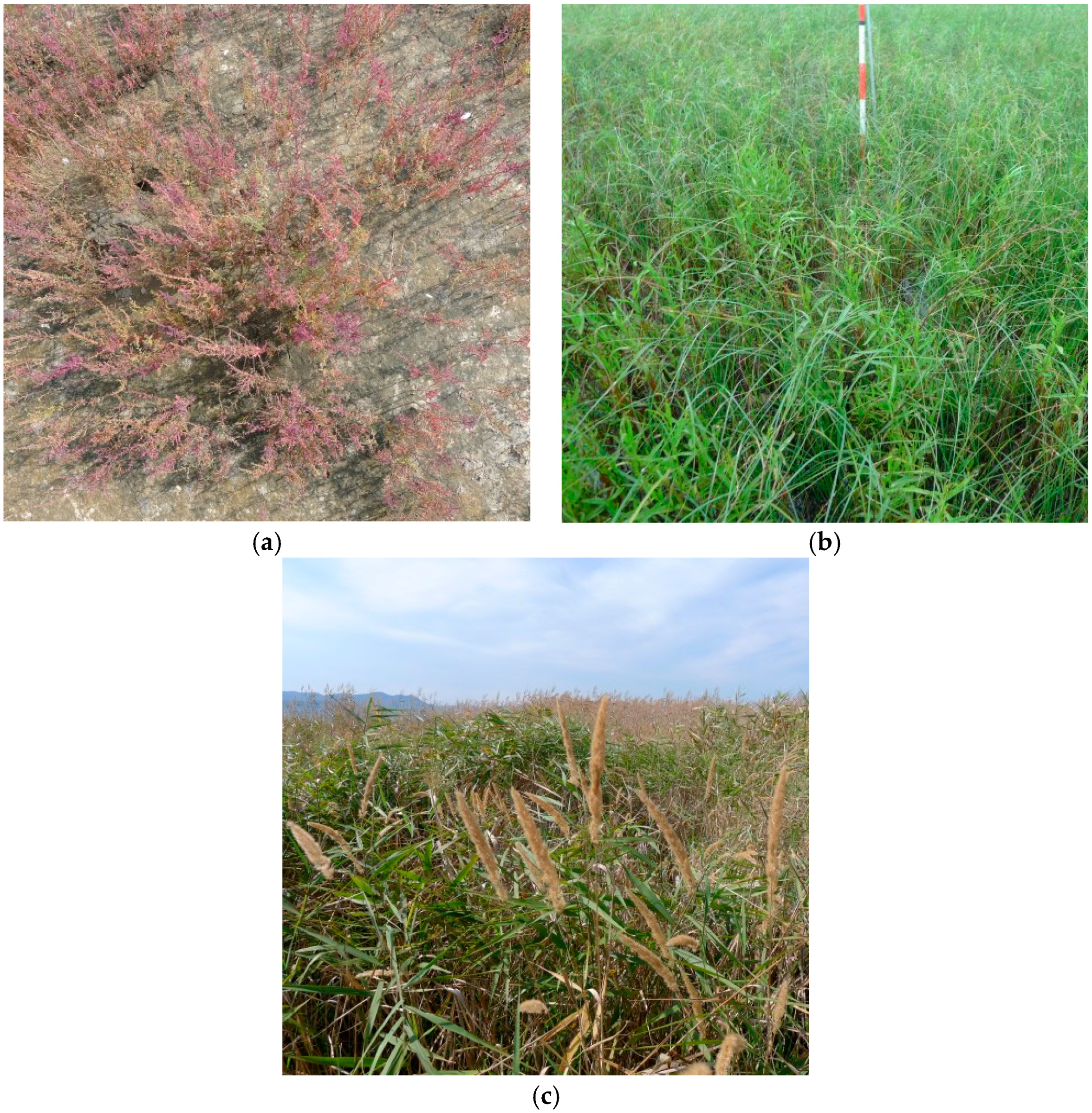
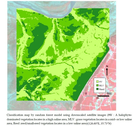
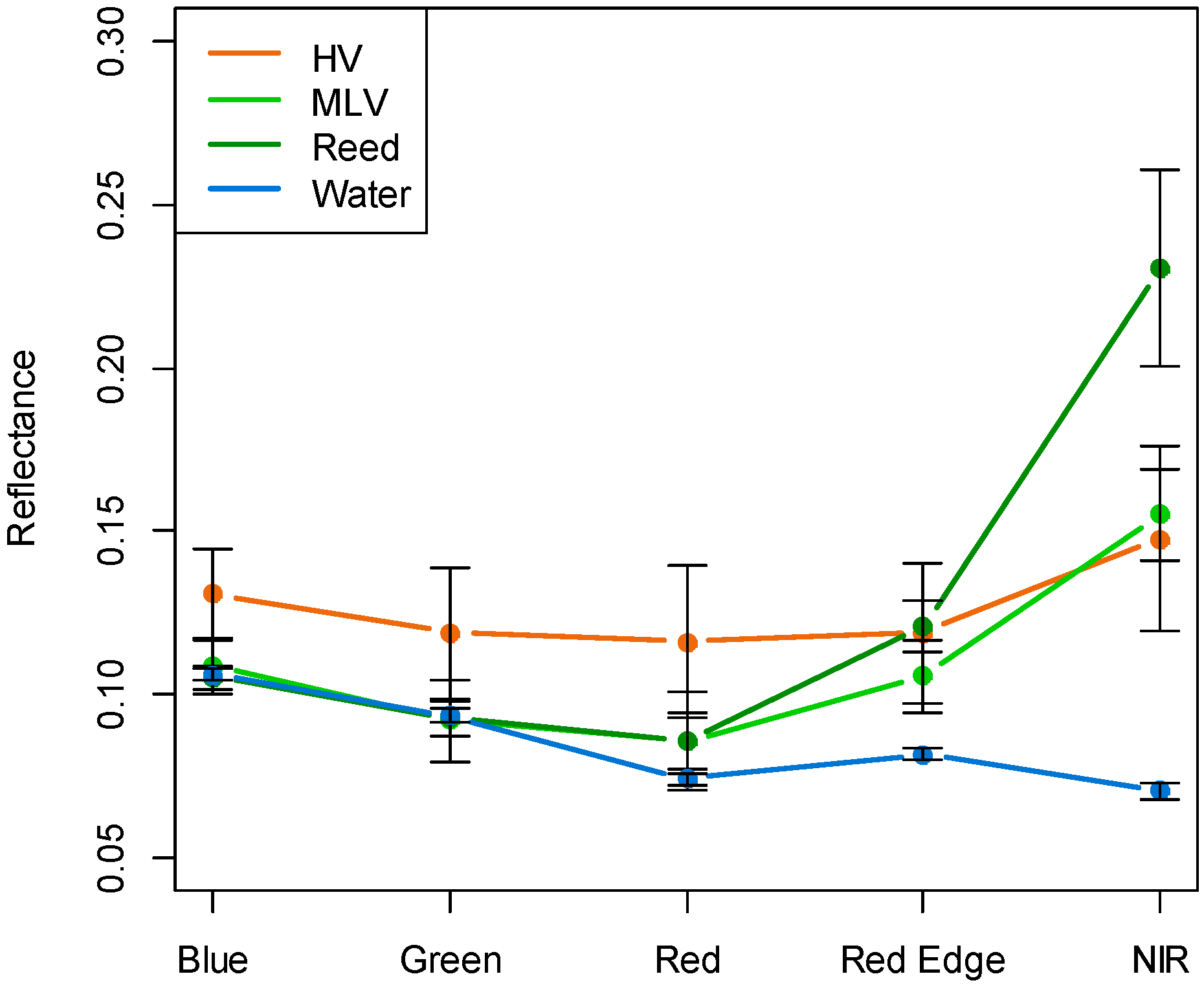
2 of the sample points and classified the typical vegetation types. There were three typical vegetation types: halophyte vegetation (HV), mid- to low saline vegetation (MLV), and reed/small-reed vegetation (Reed, Figure 3). A total of three randomly selected soil core samples (0–5 cm depth) were collected from each sample point. The soil samples, which were air dried, crushed, and uniformly mixed, were sifted through a 2 mm sieve for EC and pH analysis and a 0.5 mm sieve for organic matter content analysis. The soil EC and pH were measured in saturated paste extract and saturated paste, respectively, according to the methods described by the NAAS [28]. The organic matter content of the soils was measured by Tyurin’s method.

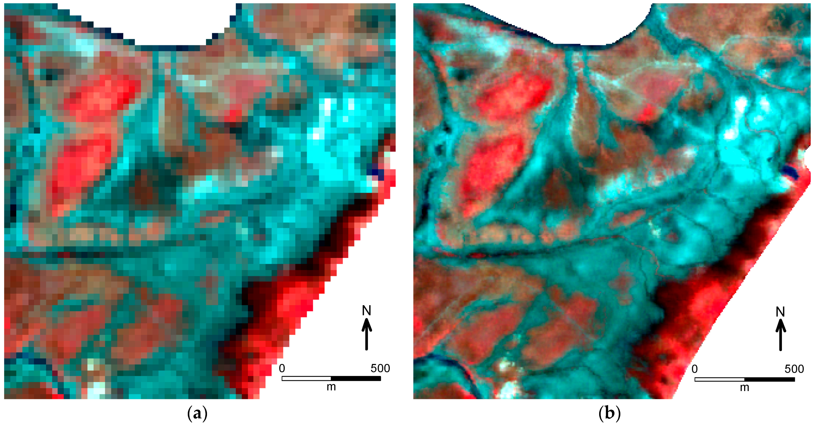
2.3. Satellite Data Acquisition and Processing

RapidEye and Landsat OLI (Operational Land Imager) satellite images were used. A RapidEye image was acquired on 1 September 2014. The RapidEye imagery is multispectral, with a red edge (690–730 nm) and blue (440–510 nm), green (520–590 nm), red (630–685 nm), and near-infrared (NIR, 760–785 nm) bands. A level 2B RapidEye image was used, and the image was georeferenced to the Universal Transverse Mercator (UTM) coordinate system using the WGS 1984 datum with an accuracy of less than the root mean square of 0.01 pixels. The image was resampled to a 6 m × 6   m spatial resolution. Image processing was conducted with ERDAS Image software (version 9.1).
Landsat 8 OLI images were acquired on 1 July and 5 October 2014. The Landsat 8 OLI blue (450–515 nm), green (525–600 nm), red (630–680 nm), and NIR (845–885 nm) bands were used for downscaling. The digital number (DN) values of the image were converted to reflectance with a multiplicative rescaling factor and an additive rescaling factor. Topographic correction was not necessary because the study area was very flat. The atmospheric correction was carried out with the Second Simulation of Satellite Signal in the Solar Spectrum (6S) model [29], using GRASS software [30].

2.4. Downscaling Cokriging

The following description of downscaling cokriging is mainly based on the work of Pardo-Iguzquiz et al. [24]. All of the formulas and notations followed Pardo-Iguzquiz et al. [24]. The cokriged finer-spatial-resolution image (downscaled Landsat) of band k, calculated from a Landsat (band k) image and RapidEye (band l), is given by:
Z ^ u k ( x 0 ) = i = 1 N λ i 0 Z V k ( x i ) + j = 1 M β j 0 Z u l ( x j )
where:
Z ^ u k ( x 0 ) is a random variable (RV) of a pixel of areal size u (RapidEye), with the spatial location x 0 and spectral band k estimated by cokriging.
Z V k ( x i ) is a RV of the pixel of the coarse spatial resolution image with areal size V (Landsat OLI) and spectral band k. N of these pixels are used. The weight assigned to the random variable of the i-th pixel is λ i 0 . The number of window pixels for Landsat (N) was nine (=3 × 3).
Z u l ( x j ) is a RV of the pixel of the fine spatial resolution image with areal size u (RapidEye) and spectral band l. M of these pixels are used. The weight assigned to the random variable of the j-th pixel is β j 0 . The number of window pixels for RapidEye (M) was 25 (=5 × 5).
The two sets of weights { λ i 0 ; i = 1,…,N} and { β j 0 ; j = 1,…,M} are obtained through cokriging. To be optimal in the sense of giving a minimum variance unbiased estimator, the sum weights of the variable Z V k must be 1 ( i = 1 N λ i 0 = 1 ), and the sum of the weights of the variable Z u l must be 0 ( j = 1 M β j 0 = 0 ). The weights are calculated by formulizing the spatial structure of the image data and minimizing the unbiased estimation variance.
There are two ways to address the local mean in the downscaling cokriging process. One is to consider non-stationarity (taking into account the variation of local mean) [26], and the other is to use a global model [24]. This study used a global model due to its ease of application and statistical reliability [24]. The point spread function (PSF) is important to consider when factoring in area-to-point kriging. A uniform PSF was applied in this study because there was little information available to formulate a specific PSF. The Fortran source code for downscaling cokriging (DISKORI) was obtained via the Computers and Geosciences website [31].

2.5. Classification of Vegetation Type

The random forest classifier (RFC) proposed by Brieman [32] was applied to image classification because it is widely used in a range of fields and often yields good results [19,33,34,35]. The random forest algorithm (RF) is a type of decision tree classification. The RFC only has two parameters: the number of trees in the forest (number of bootstrap samples from the original data) and the number of random variables at each node (the maximum number of this parameter is the number of predictors). The RFC can use diverse types of data with little restriction because it does not make specific assumptions about the data distribution. Additionally, it can easily handle a large number of input variables.
R software [36] was used for image classification. The RFC was conducted with the ‘randomForest’ package (version 4.6–10), which was implemented by Liaw and Wiener [37] based on the algorithm proposed by Brieman [32].
Classification was performed for different combinations of images (Table 1). In addition to the reflectance of image bands, the normalized difference vegetation index (NDVI) was used. The NDVI was computed with the following equation:
NDVI = ρ n i r ρ r e d ρ n i r + ρ r e d
where ρ r e d and ρ n i r are the surface reflectance at the red and near infrared band, respectively.
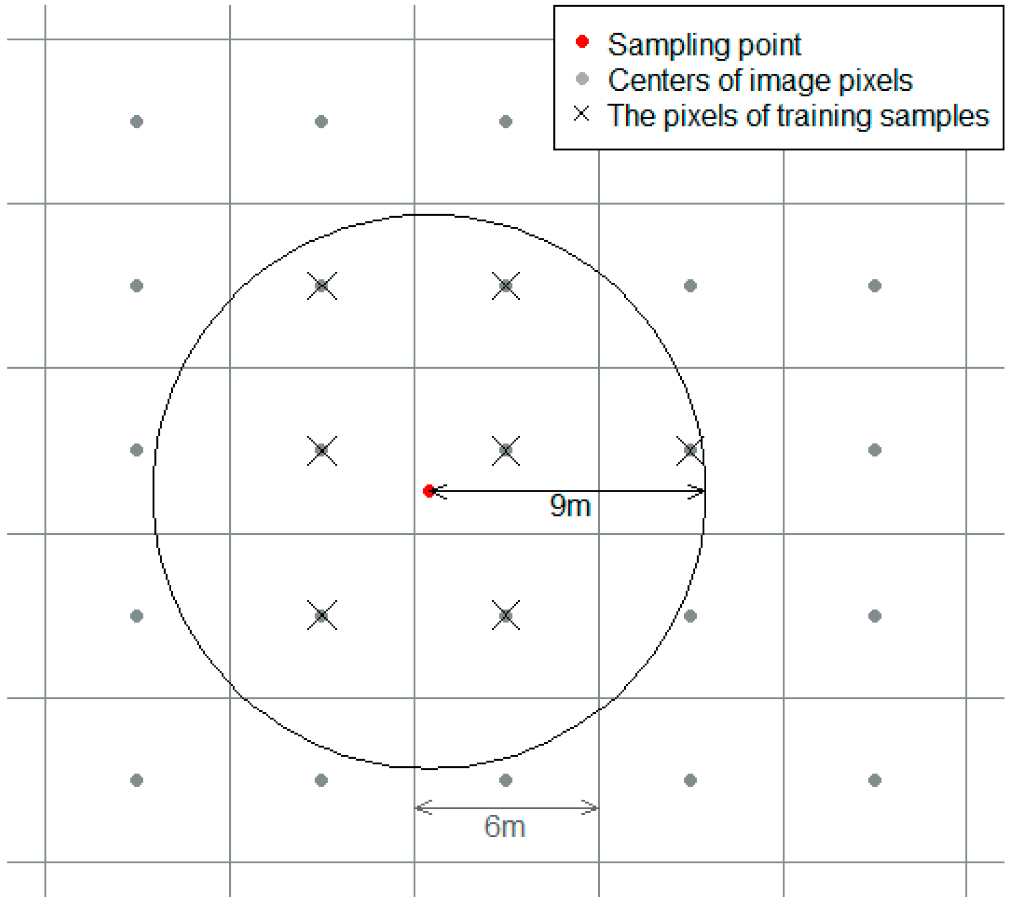
Training samples were selected, based on the 127 randomly selected field survey points. Pixels with centers within a 9 m radius of the training samples were assigned the same vegetation type as the training samples (Figure 4). The radius criterion was determined by only selecting adjacent pixels (considering the 6 m resolution of the RapidEye and downscaled Landsat imagery) to the sampling points. Diagonal pixels were selectively included, according to the distance from the sampling point. The total sample size was 915. The vegetation classification was trained using randomly selected 200 pixels from each of the three vegetation types (600 training data = 200 × three types). After building RF models, the models were used to predict the vegetation type of the remaining 315 pixels. An accuracy assessment of classifications was carried out by comparing the predicted vegetation type and field data. The confusion matrices for each model were created after classification. The overall accuracy, producer’s accuracy, user’s accuracy, and Cohens’ kappa [38] were calculated, as suggested by Congalton [39].

2.6. Characterisics of Vegetation Distribution

After creating the vegetation map, the spatial characteristics of the vegetation were analyzed with R software [36]. The mean NDVI of each vegetation type was calculated with a ‘raster’ package (version 2.5–8). The patch statistics of the vegetation types were calculated with an ‘SDMTools’ package (version 1.1–221).

3. Results

3.1. Characteristics of Vegetation Types

HV was located in the high saline area and was dominated by Suaeda spp. and/or Salicornia europaea. The plant density was generally low and very low in some locations. Although there were some areas that were rarely covered by plants, a bare soil class was not included, because it is difficult to clearly distinguish between a bare soil class and a halophyte-dominated vegetation class, due to a low plant density and biomass. Additionally, it is worth noting that the area is not degraded, but is in the process of being colonized by halophyte species. This means that the areas of low plant density will be colonized by HV in the next few years, until the condition has been eased for non-halophyte species colonization. The height of HV was less than 0.5 m. The MLV was located in the mid- or low saline areas and was dominated by diverse grass species, with an admixture of Conyza Canadensis and/or Carex scabrifolia. The height of MLV was 0.5~1.5 m. The plant density of MLV was higher than HV, but generally lower than Reed vegetation. Reed vegetation was located in the low saline area and was dominated by Phragmites communis and/or Calamagrostis epigeios. The plant density of this type was usually higher than the other types. The height of Reed vegetation was 1.5~2.5 m.

3.2. Soil Environment of Vegetation Types

The texture of all soil samples was clayey. The soil EC, pH, and organic matter (OM) of the vegetation are summarized in Table 2. The Wilcoxon rank sum test was used for the multiple comparison of mean, because the distributions were non-normal. The HV type showed the highest mean and standard deviation EC. The mean EC of the MLV and Reed vegetation types was significantly lower than HV. The high soil EC restricts the colonization of low- or non-saline plants. The pH was close to neutral in all vegetation types. However, the mean pH of HV was significantly lower than the other types. The mean OM was less than 2%. The low OM represents the poor soil conditions of the area.

3.3. Spectral Characteristics of Classification Classes

The spectral signatures of the RapidEye image are shown in Figure 5. The reflectance of the MLV and Reed classes was almost identical in the blue, green, and red bands. There was a large overlap between the HV and MLV classes in the NIR band. Although the red edge band was expected to be useful for the detection of fine differences in the vegetation condition, the three vegetation types showed a similar reflectance value in this band. The similarities in spectral reflectance among classes can reduce classification separability. However, the water class very clearly showed a distinguishable signature in the mean and standard deviation, especially in the red, red edge, and NIR bands.

3.4. Downscaling Cokriging

In this study, Landsat images with a 30 m resolution were downscaled to a 6 m resolution, to account for the spatial heterogeneity of the vegetation distribution. To conduct downscaling cokriging, the variogram and cross-variogram were fitted. An isotropic exponential model was applied as the fitting model for all variograms, because there was little difference in the direction of the experimental variogram. A nested model with two exponential structures was used, because one experimental structure was not sufficient for fitting the experimental variogram. The variogram and cross-variogram of the NIR band are shown in Figure 6. The fitted (cross) variogram models are summarized in Table 3. As the nested structure was applied, two ranges were identified. The range of the first structure was 40 m and that of the second was 300 m. In the case of the RapidEye image, the partial sills of the two structures were relatively similar. In contrast, the partial sills of the second structure were much larger than those of the first one in the Landsat image. This difference is related to the resolution of the images. For example, the small variation of the first structure can be explained by its short range. A pair of two points, separated by a smaller distance than the first range (40 m), was usually located in adjacent pixels or the same pixel. This leads to little difference in the values of the two points.
The plots of the reflectance value of the RapidEye image versus the downscaled Landsat images are shown in Figure 7. The reflectance of the July image was higher than that of the one produced in October, in all bands. However, it was lower than that of the RapidEye image in the blue and NIR bands (below of 1:1 line). The reflectance of the October image was more highly correlated with the RapidEye image in all bands.
Figure 8 and Figure 9 show the original Landsat images and downscaled images. Downscaled images provide spatially detailed information, especially in terms of the linear shape. The difference in the phenological traits of vegetation is easily found in these multi-temporal images. The color change of the images was variable, according to the location. Some areas remained unchanged or underwent little change, while other areas changed in color.

3.5. Result of Image Classification

The RFC was used to test whether the number of trees (the size of the forest) or the number of variables investigated at each node affected the classification accuracy. The former did not create a significant change in the results when the number of trees was larger than 1000. The accuracy was also not substantially affected by the number of variables investigated at each node when the number of trees was larger than 1000. The RFC was carried out with 1000 trees and two variables were investigated at each node.
A total of six RF models (Table 1) were tested for vegetation classification accuracy. The results are shown in Table 4, Table 5, Table 6, Table 7, Table 8 and Table 9. The RF model (Model 1) that used a single RapidEye image yielded a poorer result (Overall Accuracy (OA) = 82.5%) than a multi-temporal image, which improved accuracy. Two images (RF model 2 (OA = 88.3%) and RF model 3 (OA = 87.9%)) were more efficient at producing accurate results. However, the best result was shown in the later three RF models (RF model 4–6) that used three image data, especially the RapidEye and Landsat images acquired in July and October, without the Rededge band (RF model 6 (OA = 92.4%) Table 9). There was no substantial difference in OA and K ^ among the three RF models.
The classification map of the RF model 6 is shown in Figure 10. The Reed patches were surrounded by MLV, and HV shared most of its boundaries with MLV. This pattern of vegetation distribution implies that there is a strong environmental gradient that has been spatially structured and regulates the vegetation distribution. Additionally, there were many linear patches located along narrow channels that were naturally formed when the area was an estuarine tidal flat.
The percentage of each vegetation type was 39.8% (HV), 38.9% (MLV), and 21.3% (Reed) (Table 10). Almost 40% of the total area was covered by halophyte-dominated vegetation. Another 40% was colonized by diverse grass/herbaceous plants. The rest of the area was occupied by relatively dense vegetation, such as reed and small-reed plants. However, the Reed class is prone to expand due to its rhizome roots system, which is competitive in grass/herbaceous communities.
The pattern of NDVI reflects the plant phenology. Early July marks the beginning of the growing season. The leaf biomass increases until late summer or early autumn. After the peak, the NDVI decreases, due to the loss of leaf biomass. The pattern was the same for all vegetation types (Table 10). The Reed type had the highest NDVI, meaning that the Reed type may substantially contribute to the above ground biomass of the area, regardless of its relatively small coverage.
The area of the vegetation patch was calculated and the frequency is shown in Figure 11. There were many small patches. The number of patches smaller than 450 m2 (half of Landsat support area: 30 m × 30 m) was 569. These small patches are difficult to identify using the Landsat image for the vegetation classification. Each pixel of Landsat was composed of 25 subpixels that contained information on the vegetation types. Among the Landsat pixels, only 47.7% were composed of a single vegetation type, 44.6% were composed of two vegetation types, and 7.7% were composed of three vegetation types. The highly diverse vegetation distribution needs finer image data to figure out the state of vegetation distribution.

4. Discussion

The study area became permanent land after the water level was lowered in 2010, and the soil condition has been changing. Kim et al. [3] reported the mean soil EC of halophyte vegetation as 14 dSm-1, mixed vegetation as 6.7 dSm-1, and reed dominant vegetation as 3.0 dSm-1 in 2010. Compared to an earlier study, the soil EC showed lower levels in 2014. The mean soil EC of HV was 9.5 dSm-1, MLV was 1.0 dSm-1, and Reed was 0.5 dSm-1. The rapid changes in the soil conditions during this relatively short period also influenced the distribution of vegetation.
Although the characteristics and distribution of vegetation are crucial for determining the condition of the ecosystem, it is hard to create accurate vegetation maps of grass/herbaceous plant-dominated areas. There have been a number of studies that have tried to improve the accuracy of vegetation mapping using the phenological characteristics of plants [11,20,21,22]. Gilmore [11] suggested that it is possible to discriminate Phragmites spp. using single-date images acquired in the autumn season. However, it was difficult to classify Phragmites-dominated vegetation using timely acquired RapidEye imagery. More than 20% of the Reed class was misclassified (Table 4). The accuracy increased when the multi-temporal images were used in classification (Table 5, Table 6, Table 7 and Table 8).
The goal is to acquire multi-temporal images, especially in the growing season. This research applied cokriging to downscale Landsat imagery, which is easy to obtain, but has limited utility due to its relatively low spatial resolution. Sharpened Landsat imagery taken at different time periods improved the accuracy of the vegetation map. Cokriging is a useful approach because it is based on a well-established geostatistical theory and provides a framework to combine different types of data [23,24]. However, the application of the approach has been limited, until recently [40]. The results show that image downscaling using cokriging can be applied in vegetation studies and is useful for the analysis of multi-temporal data.
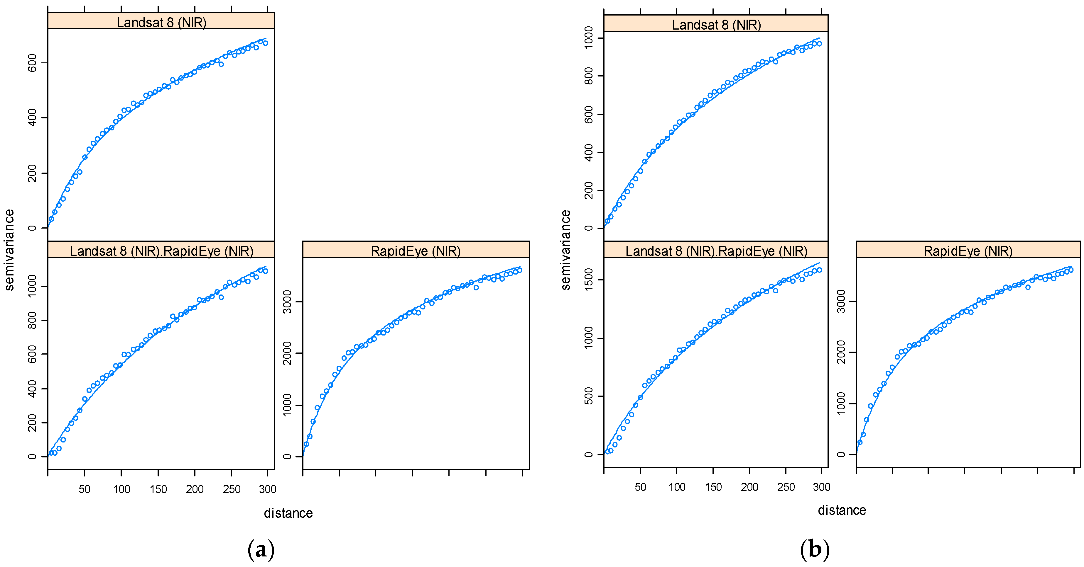
In this study, a nested variogram model with two structures was used in cokriging. A nested model is useful for modelling the spatial structure with different scales [41,42]. Pardo-Iguzquiz et al. [24] also used a nested model for downscaling two images with different resolutions. The nested structure model fitted the data well, with a 0 nugget value. The partial sill of the first structure (short range) was much smaller than that of the second structure in a variogram model of a low resolution image. It is consistent with the results of this study. However, in both cases, further research is needed to quantify the uncertainty of using the nested model for downscaling images.
Multi-temporal and multispectral data analysis raises the problem that the number of input variables can rapidly increase. The RFC can easily and effectively handle a large number of input variables [19,33,34,43]. For that reason, it was used in this study and yielded good results.

5. Conclusions

An area reclaimed from estuarine tidal flats forms a very unique and dynamic ecosystem. The creation of a large reclamation area in itself is a difficult challenge for ecosystem monitoring and management.
This paper presents a novel approach for the classification of vegetation in reclaimed areas, using multi-temporal downscaled Landsat imagery along with RapidEye imagery. The study area has a typical environmental gradient of soil salinity and vegetation types, of which the distribution is mainly controlled by the environmental conditions. This study provides a framework to reduce spatial and temporal resolution by downscaling images with a low spatial and high temporal resolution, with an image that has a high spatial and low temporal resolution. Multi-temporal downscaled images were compared to single high resolution images, to classify the vegetation type. The accuracy of the vegetation map using the multi-temporal downscaled image was approximately 10% higher than the accuracy of the map using a single high resolution image.
These results demonstrate that the downscaling technique is useful when a high resolution image is not available. This technique is also capable of increasing the utility of relatively low spatial resolution images, such as Landsat imagery. The results also confirmed the performance of the RFC. The analysis of multi-temporal multi-band data causes difficulties in handling high dimensional data. The RFC was very versatile and demonstrated a high performance when classifying the vegetation type with a large number of variables.
The results of this study can be utilized in ecosystem monitoring for target objects that are difficult to distinguish with single, high spatial resolution imagery. The method can not only expand the time span of the data, but also increase the accuracy of mapping. It is also possible to apply this approach to the monitoring of ecosystems that witness rapid changes.

Acknowledgments

The authors thank Kyung Hyun Kim, Young-Joo Ko, Dal-Ho Kim, and Xinmei Jin for their enthusiastic assistance in the field survey. This research was funded by the Korea Aerospace Research Institute.

Author Contributions

Mu-Sup Beon designed and coordinated the research and participated in the analysis and interpretation of the results. Ki Hwan Cho designed the research and collected the field data, and participated in the analysis and interpretation of the results. Hyun Ok Kim participated in the analysis and interpretation of the results, and Hyun-Kyung Oh participated in the field work. Jong-Chul Jeong participated in the analysis and interpretation of the results. All of the authors contributed to the preparation and revision of this paper.

Conflicts of Interest

The authors declare no conflict of interest

References

  1. Kim, S.; Jeong, J.-H.; Choi, W.-Y.; Lee, J.-H.; Lee, K.-B.; Im, I.-B. Change of vegetation characteristics and soil chemical properties at Saemangeum reclaimed land in Korea. Weed Turfgrass Sci. 2013, 2, 260–266. [Google Scholar] [CrossRef]
  2. Lee, S.-H.; An, Y.; Yoo, S.-H.; Lee, S.-M. Changes in Early Stage Vegetation Succession as Affected by Desalinization Process in Dae-Ho Reclaimed Land. Korean J. Environ. Agric. 2000, 19, 364–369. [Google Scholar]
  3. Kim, S.; Kim, T.-K.; Jeong, J.-H.; Yang, C.-H.; Lee, J.-H.; Choi, W.-Y.; Kim, Y.-D.; Kim, S.-J.; Seong, K.-Y. Characteristics of vegetation on soils having different salinity in recently reclaimed Saemangeum in region of Korea. Korean J. Weed Sci. 2012, 32, 1–9. [Google Scholar] [CrossRef]
  4. Lee, S.-H.; Ji, K.-J.; An, Y.; Ro, H.-M. Soil salinity and vegetation distribution at four tidal reclamation project areas. Korean J. Environ. Agric. 2003, 22, 79–86. [Google Scholar]
  5. Kang, B.-H.; Shim, S.-I. Screening of saline tolerant plants and development of biological monitoring technique for saline strees. 1. Survey of vegetation in saline region and determination of saline tolerance of the plant species of the region. Korean J. Environ. Agric. 1998, 17, 26–33. [Google Scholar]
  6. Jeong, J.-C. The analysis of temporal and spatial variation on the vegetation area of the Siwha tidal flat. J. Environ. Impact Assess. 2011, 20, 349–356. [Google Scholar]
  7. Jeong, J.-C. The satellite observation for spatial changes of vegetation in Saemangum tidal flat. J. Environ. Impact Assess. 2014, 23, 150–156. [Google Scholar] [CrossRef]
  8. Kim, C.H.; Lee, K.B.; Kim, J.D.; Cho, T.D.; Kim, M.S. The study on the flora and vegetation of salt marshes of Dongin-river estuary in Jeonbuk. J. Korean Environ. Sci. Soc. 2005, 14, 817–825. [Google Scholar]
  9. Oh, H.-K.; Kim, S.-C.; You, J.-H. Halophytes and vegetation of Seocheon tidal flat wetland conservation area. J. Environ. Impact Assess. 2013, 22, 409–426. [Google Scholar] [CrossRef]
  10. Shim, H.-B.; Cho, W.-B.; Choi, B.-H. Distribution of halophytes in coastal salt marsh and on sand dunes in Korea. Korean J. Plant Taxon. 2009, 39, 264–276. [Google Scholar]
  11. Gilmore, M.S.; Wilson, E.H.; Barrett, N.; Civco, D.L.; Prisloe, S.; Hurd, J.D.; Chadwick, C. Integrating multi-temporal spectral and structural information to map wetland vegetation in a lower Connecticut River tidal marsh. Remote Sens. Environ. 2008, 112, 4048–4060. [Google Scholar] [CrossRef]
  12. Wang, C.; Menenti, M.; Stoll, M.-P.; Belluco, E.; Marani, M. Mapping mixed vegetation communities in salt marshes using airborne spectral data. Remote Sens. Environ. 2007, 107, 559–570. [Google Scholar] [CrossRef]
  13. Belluco, E.; Camuffo, M.; Ferrari, S.; Modenese, L.; Silvestri, S.; Marani, A.; Marani, M. Mapping salt-marsh vegetation by multispectral and hyperspectral remote sensing. Remote Sens. Environ. 2006, 105, 54–67. [Google Scholar] [CrossRef]
  14. Marani, M.; Belluco, E.; Ferrari, S.; Silvestri, S.; D’Alpaos, A.; Lanzoni, S.; Feola, A.; Rinaldo, A. Analysis, synthesis and modelling of high-resolution observations of salt-marsh eco-geomorphological patterns in the Venice lagoon. Estuar. Coast. Shelf Sci. 2006, 69, 414–426. [Google Scholar] [CrossRef]
  15. Sadro, S.; Gastil-Buhl, M.; Melack, J. Characterizing patterns of plant distribution in a Southern California salt marsh using remotely sensed topographic and hyperspectral data and local tidal fluctuations. Remote Sens. Environ. 2007, 110, 226–239. [Google Scholar] [CrossRef]
  16. Schmidt, K.S.; Skidmore, A.K. Spectral discrimination of vegetation types in a coastal wetland. Remote Sens. Environ. 2003, 85, 92–108. [Google Scholar] [CrossRef]
  17. Gao, Z.G.; Zhang, L.Q. Multi-seasonal spectral characteristics analysis of coastal salt marsh vegetation in Shanghai, China. Estuar. Coast. Shelf Sci. 2006, 69, 217–224. [Google Scholar] [CrossRef]
  18. Lee, K.-D.; Baek, S.-C.; Hong, S.-Y.; Kim, Y.-H.; Na, S.-I.; Lee, K.-B. Classification of soil desalination areas using high resolution satellite imagery in Saemangeum reclaimed land. Korean J. Soil Sci. Fertil. 2013, 46, 426–433. [Google Scholar] [CrossRef]
  19. Beijma, S.V.; Comber, A.; Lamb, A. Random forest classification of salt marsh vegetation habitats using quad-polarimetric airborne SAR, elevation and optical RS data. Remote Sens. Environ. 2014, 149, 118–129. [Google Scholar] [CrossRef]
  20. Denninson, P.E.; Roberts, D.A. The effects of vegetation phenology on endmember selection and species mapping in southern California chaparral. Remote Sens. Environ. 2003, 87, 295–309. [Google Scholar] [CrossRef]
  21. Key, T.; Warner, T.A.; McGraw, J.B.; Fajvan, M.A. A comparision of multispectral and multitemoral information in high spatial resolution imagery for classification of individual tree species in a temperate hardwood forest. Remote Sens. Environ. 2001, 75, 100–112. [Google Scholar] [CrossRef]
  22. Reed, B.C.; Brown, J.F.; VanderZee, D.; Loveland, T.R.; Merchant, J.W.; Ohlen, D.O. Measuring phenological variability from satellite imagery. J. Veg. Sci. 1994, 5, 703–714. [Google Scholar] [CrossRef]
  23. Atkinson, P.M. Downscaling in remote sensing. Int. J. Appl. Earth Obs. Geoinf. 2013, 22, 106–114. [Google Scholar] [CrossRef]
  24. Pardo-Iguzquiza, E.; Chica-Olmo, M.; Atkinson, P.M. Downscaling cokriging for image sharpening. Remote Sens. Environ. 2006, 102, 86–98. [Google Scholar] [CrossRef]
  25. Pardo-Iguzquiza, E.; Atkinson, P.M. Modelling the semivariograms and cross-variograms required in downscaling cokriging by numerical convolution-deconvolution. Comput. Geosci. 2007, 33, 1273–1284. [Google Scholar] [CrossRef]
  26. Pardo-Iguzquiza, E.; Rodriguez-Galiano, V.F.; Chica-Olmo, M.; Atkinson, P.M. Image fusion by spatially adaptive filtering using downscaling cokriging. ISPRS J. Photogramm. Remote Sens. 2011, 66, 337–346. [Google Scholar] [CrossRef]
  27. Ministry of Land Transport and Maritime Affairs (MLTMA). Stabilized Grantee Scheme for Dredging Reclamation Soil in Saemangeum Area; Publication No. 11-1611000-001718-01; MLTMA: Gwacheon, Korea, 2011.
  28. National Academy of Agricultural Science (NAAS). Methods of Soil Chemical Analysis; National Academy of Agricultural Science, Rural Development Administration: Suwon, Korea, 2010. [Google Scholar]
  29. Vermote, E.F.; Tanre, D.; Deuze, J.L.; Herman, M.; Morcrette, J.J. Second simulation of the satellite signal in the solar spectrum, 6S: An overview. IEEE Trans. Geosci. Remote Sens. 1997, 35, 675–686. [Google Scholar] [CrossRef]
  30. GRASS Development Team. Geographic Resources Analysis Support System (GRASS) Software, version 7.0; Open Source Geospatial Foundation. Available online: http://grass.osgeo.org (accessed on 10 December 2016).
  31. Pardo-Iguzquiza, E.; Atkinson, P.M.; Chica-Olmo, M. Dscokri: A library of computer programs for downscaling cokriging in support of remote sensing applications. Comput. Geosci. 2010, 36, 881–894. [Google Scholar] [CrossRef]
  32. Breiman, L. Random forest. Mach. Learn. 2001, 45, 5–32. [Google Scholar] [CrossRef]
  33. Concoran, J.; Knight, J.; Gallant, A. Influence of multi-source and multi-temporal remotely sensed and ancillary data on the accuracy of random forest classification of wetlands in northern Minnesota. Remote Sens. 2013, 5, 3212–3238. [Google Scholar] [CrossRef]
  34. Cutler, D.R.; Thomas, C.; Edwards, J.; Beard, K.H.; Cutler, A.; Hess, K.T. Random forests for classification in ecology. Ecology 2007, 88, 2783–2792. [Google Scholar] [CrossRef]
  35. Feng, Q.; Gong, J.; Liu, J.; Li, Y. Monitoring cropland dynamics of the yellow river delta base on multi-temporal landsat imagery over 1986 to 2015. Sustainability 2015, 7, 14834–14858. [Google Scholar] [CrossRef]
  36. R Core Team. R: A Language and Environment for Statistical Computing. R Foundation for Statistical Computing: Vienna, Austria. Available online: https://www.R-project.Org (accessed on 10 December 2016).
  37. Liaw, A.; Wiener, M. Classification and regression by randomforest. R News 2002, 2, 18–22. [Google Scholar]
  38. Cohen, J. A coefficient of aggreement for nominal scales. Educ. Psychol. Meas. 1960, 20, 37–46. [Google Scholar] [CrossRef]
  39. Congalton, R.G. A review of assessing the accuracy of classification of remotely sensed data. Remote Sens. Environ. 1991, 37, 35–46. [Google Scholar] [CrossRef]
  40. Tang, Y.; Atkinson, P.M.; Zhang, J. Downscaling remotely sensed imagery using area-to-point cokriging and multiple-point geostatistical simulation. ISPRS J. Photogramm. Remote Sens. 2015, 101, 174–185. [Google Scholar] [CrossRef]
  41. Gelfand, A.E.; Banerjee, S. Multivariate spatial process models. In Handbook of Spatial Statistics; Gelfand, A.E., Diggle, P.J., Fuentes, M., Guttorp, P., Eds.; Chapman & Hall/CRC: Boca Raton, FL, USA, 2010; pp. 495–515. [Google Scholar]
  42. Chiles, J.; Delfiner, P. Geostatistics: Modeling Spatial Uncertainty; Wiley: New York, NY, USA, 1999. [Google Scholar]
  43. Lowe, B.; Kulkarni, A. Multispectral image analysis using random forest. Int. J. Soft Comput. 2015, 6, 1–14. [Google Scholar] [CrossRef]
Figure 1. Overview of the Saemangeum area: (a) 1 June 2009, 4-3-2 Landsat 5; (b) 5 October 2014, 5-4-3 Landsat 8. The EL is maintained at approximately −1.5 m; insets show the location of the study area in Figure 2.
Remotesensing 09 00272 g001
Figure 2. 1 September 2014, 5-3-2 RapidEye image of the study area; (a) southern part of the Saemangeum; (b) study area and 127 randomly selected sample points.
Remotesensing 09 00272 g002
Figure 3. The typical vegetation types in Saemangeum, (a) HV dominated by Suaeda spp.; (b) MLV dominated by Aster tripolium and Carex scabrifolia; (c) Reed dominated by Phragmites communis and Calamagrostis epigeios.
Remotesensing 09 00272 g003
Figure 4. A diagram of training samples.
Remotesensing 09 00272 g004
Figure 5. Spectral signatures of training data (RapidEye image). Dot and error bar represents the mean and standard deviation of reflectance, respectively.
Remotesensing 09 00272 g005
Figure 6. The variogram and cross-variogram between the Landsat 8 NIR band and RapidEye NIR band (image value = Reflectance × 1000). (a) Landsat (1 July); (b) Landsat (5 October).
Remotesensing 09 00272 g006
Figure 7. Scatter plots of RapidEye reflectance vs. downscaled Landsat reflectance. The correlation coefficient between the values of RapidEye and downscaled Landsat are shown in the r value.
Remotesensing 09 00272 g007
Figure 8. (a) Original Landsat image (1 July 2014, 5-4-3) and (b) images downscaled by cokriging (126.60°E, 35.73ºN).
Remotesensing 09 00272 g008
Figure 9. (a) Original Landsat image (5 October 2014, 5-4-3) and (b) images downscaled by cokriging (126.60°E, 35.73ºN).
Remotesensing 09 00272 g009
Figure 10. Classification map by the RF model 6 (126.60°E, 35.73°N).
Remotesensing 09 00272 g010
Figure 11. Histogram of the vegetation patch area (m2).
Remotesensing 09 00272 g011
Table 1. Image bands used for classification.
Input ImagesRF Model
123456
RapidEye
1 Sepetember
BlueOOOOOO
GreenOOOOOO
RedOOOOOO
Red edgeOOOOO
NIROOOOOO
NDVIOOO OO
Downscaled Landsat
1 July
Blue O OOO
Green O OOO
Red O OOO
NIR O OOO
NDVI O OO
Downscaled Landsat
5 October
Blue OOOO
Green OOOO
Red OOOO
NIR OOOO
NDVI O OO
Table 2. Environmental conditions of sample points according to the vegetation types. Means with different superscript letters indicate significant difference between vegetation types (p < 0.05). (Mean: Arithmetic mean, SD: Standard deviation)
HVMLVReed
MeanSDMeanSDMeanSD
EC (dS/m)9.7 a5.51.3 b2.10.5 b0.4
pH7.3 b0.57.8 a0.67.6 a0.4
OM (%)1.7 a0.41.6 a0.42.0 a1.1
Table 3. Variogram models used in downscaling cokriging.
RapidEye (1 Sepetember)Landsat (1 July)Cross-Variogram
NuggetFirst StructureSecond StructureNuggetFirst StructureSecond StructureNuggetFirst StructureSecond Structure
Common Range 40300 40300 40300
Partial SillBlue019527001027005260
Green0340300030490030350
Red0470390060800030510
NIR01540342001808100751660
RapidEye (1 Sepetember)Landsat (5 October)Cross-Variogram
NuggetFirst StructureSecond StructureNuggetFirst StructureSecond StructureNuggetFirst StructureSecond Structure
Common Range 40300 40300 40300
Partial SillBlue0195270010110020185
Green0340300025230045320
Red0470390040285085370
NIR0154034200155135001902325
Table 4. Confusion matrix of the RF model using RapidEye (RF model 1).
K ^ = 0.72Reference
HVMLVReedUser’s Accuracy
PredictionHV11214188.2%
MLV7108887.8%
Reed0254061.5%
Producer’s accuracy94.1%73.5%81.6%82.5%
Table 5. Confusion matrix of the RF model using RapidEye and Landsat (1 July) (RF model 2).
K ^ = 0.81Reference
HVMLVReedUser’s Accuracy
PredictionHV11515088.5%
MLV3120693.0%
Reed1124376.8%
Producer’s accuracy96.6%81.6%87.8%88.3%
Table 6. Confusion matrix of the RF model using RapidEye and Landsat (5 October) (RF model 3).
K ^ = 0.81Reference
HVMLVReedUser’s Accuracy
PredictionHV11312189.7%
MLV6120492.3%
Reed0154474.6%
Producer’s accuracy95.0%81.6%89.8%87.9%
Table 7. Confusion matrix of the RF model using all of the bands, excluding NDVI (RF model 4).
K ^ = 0.87Reference
HVMLVReedUser’s Accuracy
PredictionHV11513089.8%
MLV4129494.2%
Reed054590.0%
Producer’s accuracy96.6%87.8%91.8%91.7%
Table 8. Confusion matrix of the RF model using all of the bands (RF model 5).
K ^ = 0.87Reference
HVMLVReedUser’s Accuracy
PredictionHV11412090.5%
MLV5131493.6%
Reed044591.8%
Producer’s accuracy95.8%89.1%91.8%92.1%
Table 9. Confusion matrix of the RF model using all of the bands, excluding Red Edge band (RF model 6).
K ^ = 0.88Reference
HVMLVReedUser’s Accuracy
PredictionHV11410091.9%
MLV5133593.0%
Reed044491.7%
Producer’s accuracy95.8%90.5%89.8%92.4%
Table 10. Zonal statistics of each vegetation type.
HVMLVReed
Area (%)39.838.921.3
Mean NDVI1 July (Downscaled Landsat 8)0.1880.2810.463
1 Sepetember (Rapid Eye)0.2620.4410.527
5 October (Downscaled Landsat 8)0.2160.3890.491

