
Spatio-Temporal Change of Lake Water Extent in Wuhan Urban Agglomeration Based on Landsat Images from 1987 to 2015


 , and
, and
Abstract
:
1. Introduction
2. Materials
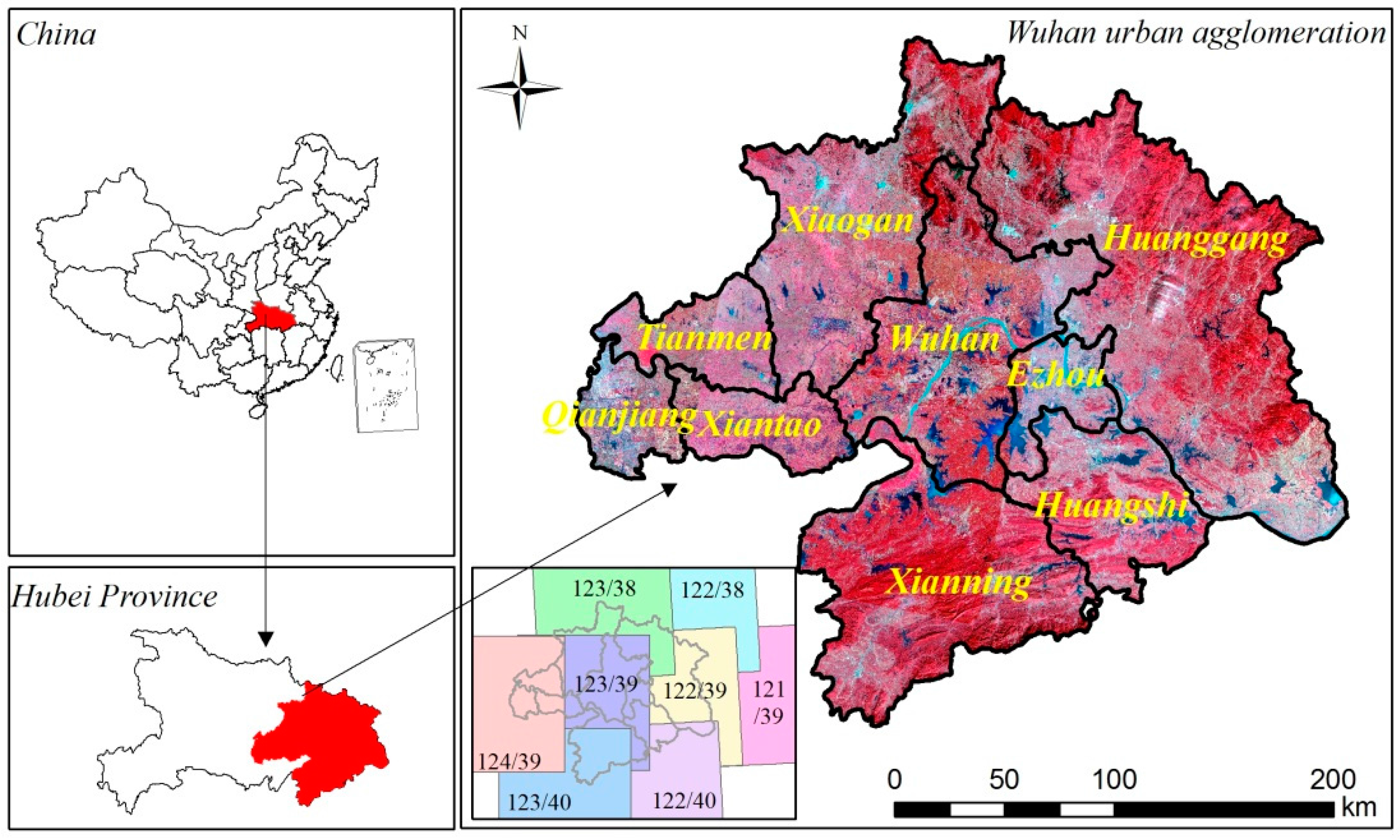
2.1. Study Area
2.2. Study Data
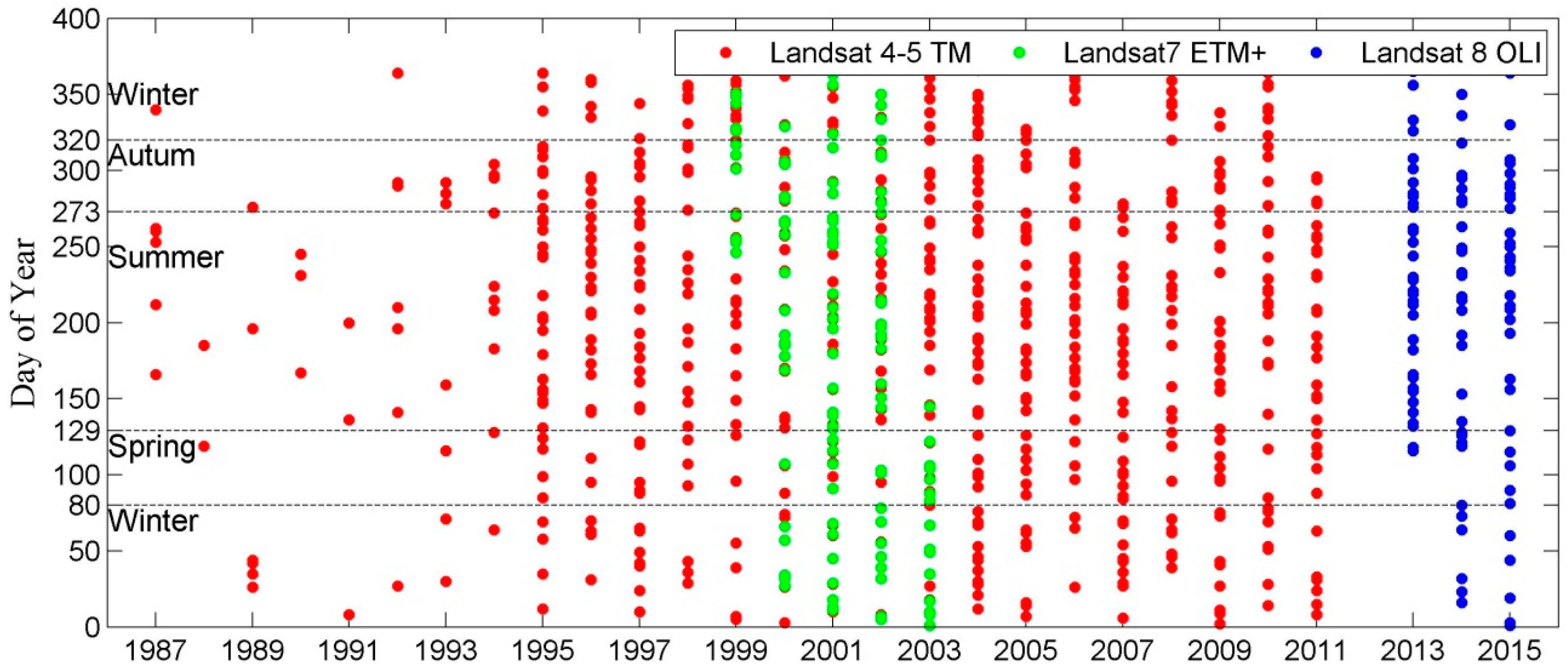
2.2.1. Landsat Time Series
2.2.2. Landuse, Precipitation and DEM data
3. Methods
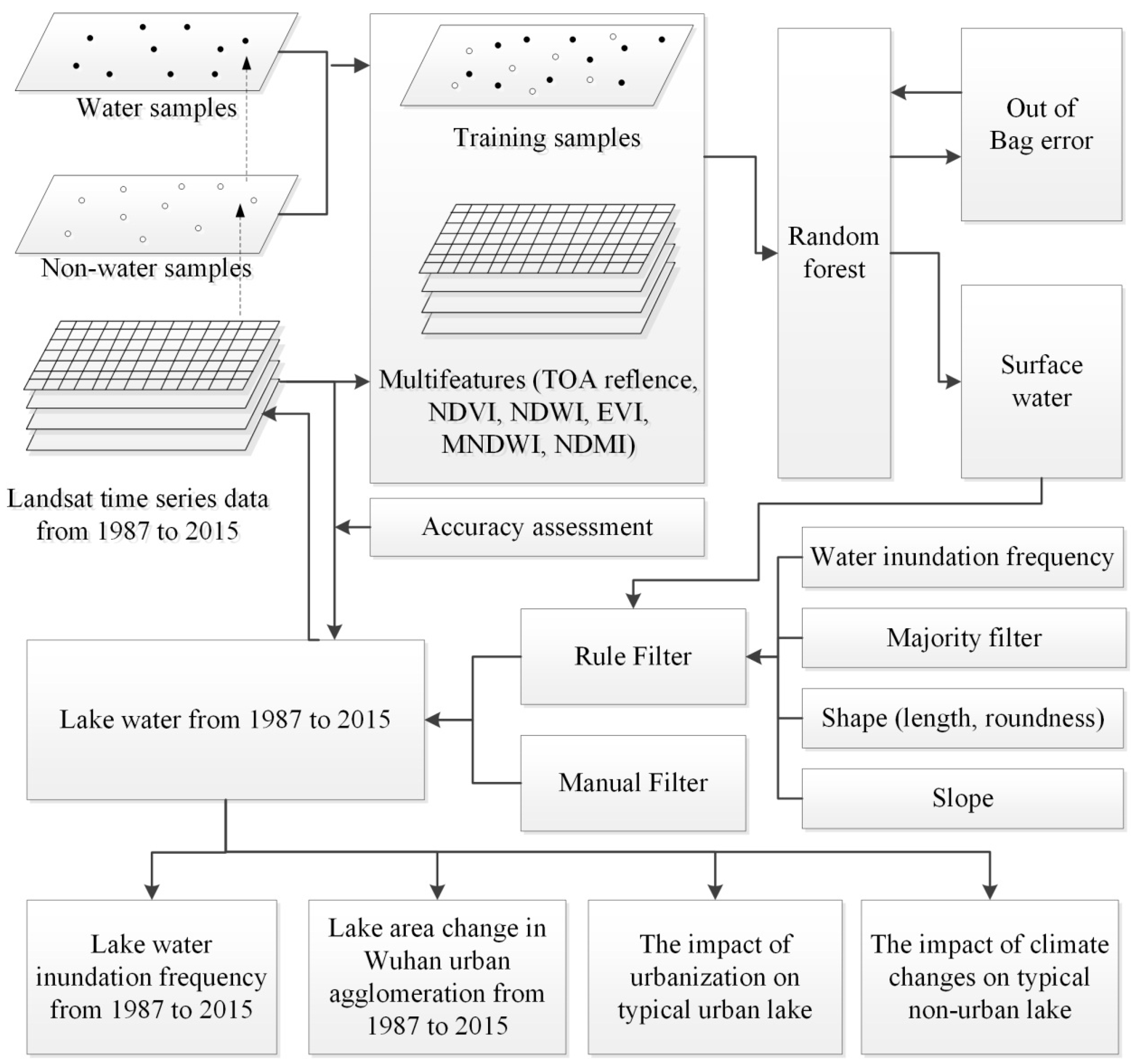
3.1. Flowchart
3.2. Collection of Feature Variables
3.3. Collection of Training Samples
3.4. Image Classification Based on Random Forest Model
3.5. Extracting Lakes Based on Shape Features and Water Inundation Frequency
3.6. Accuracy Assessment of Extracted Lakes
4. Results
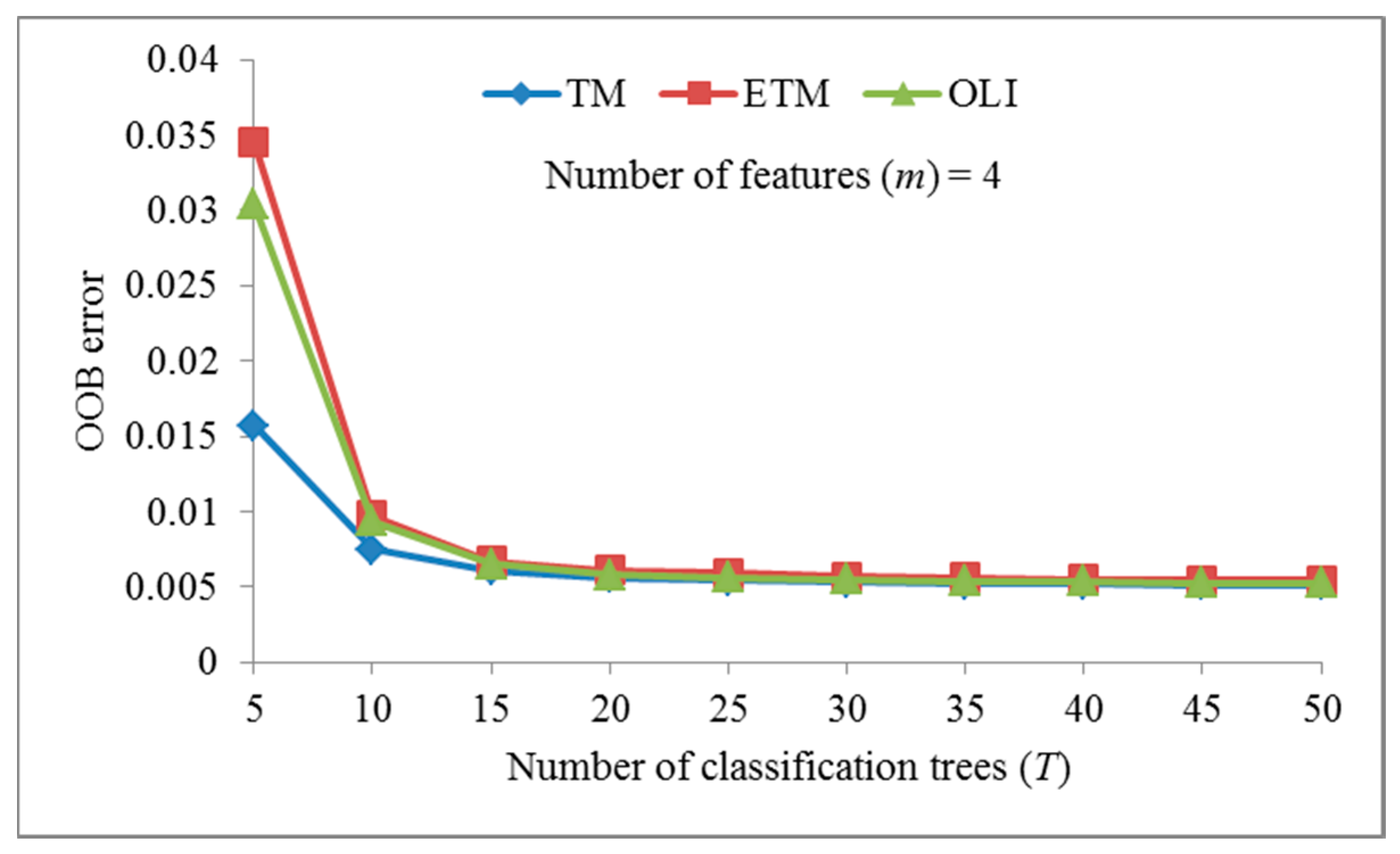
4.1. Determining Optimal Classification Trees
4.2. Accuracy of the Extracted Lakes
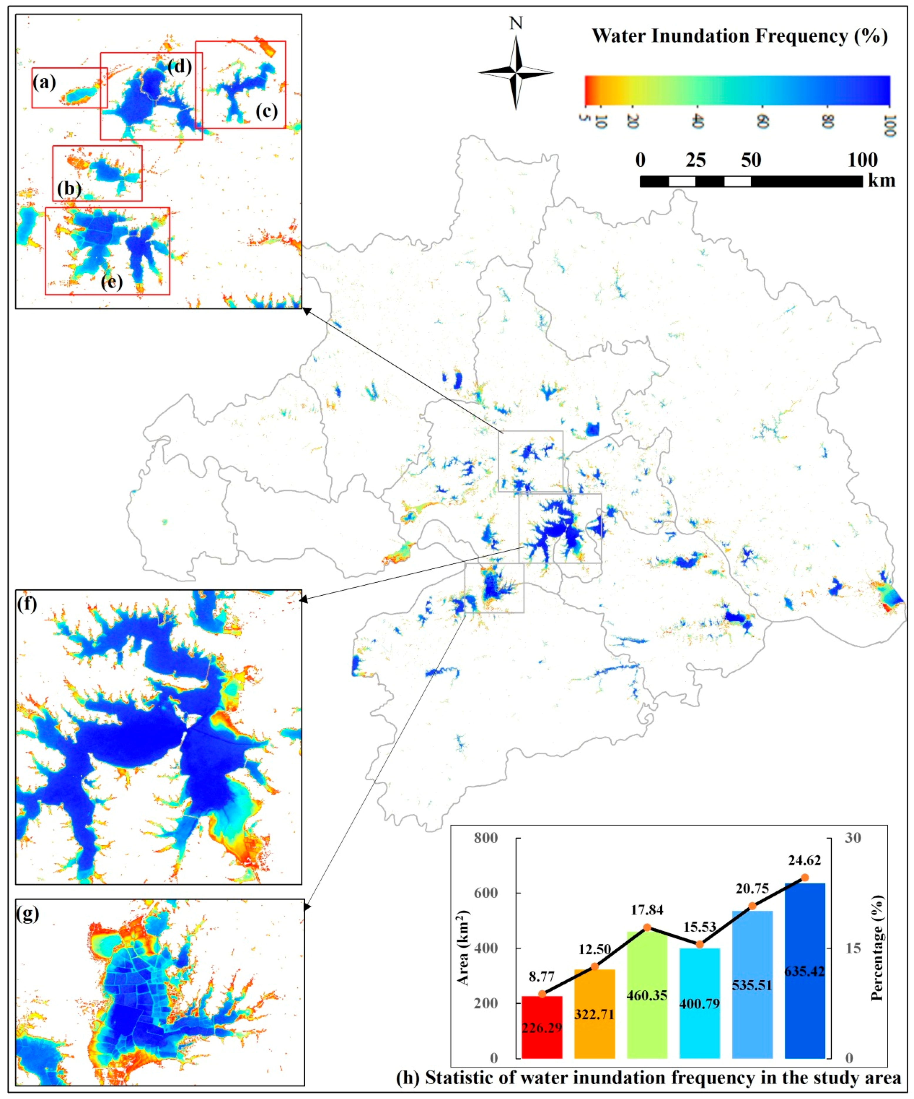
4.3. Water Inundation Frequency from 1987 to 2015
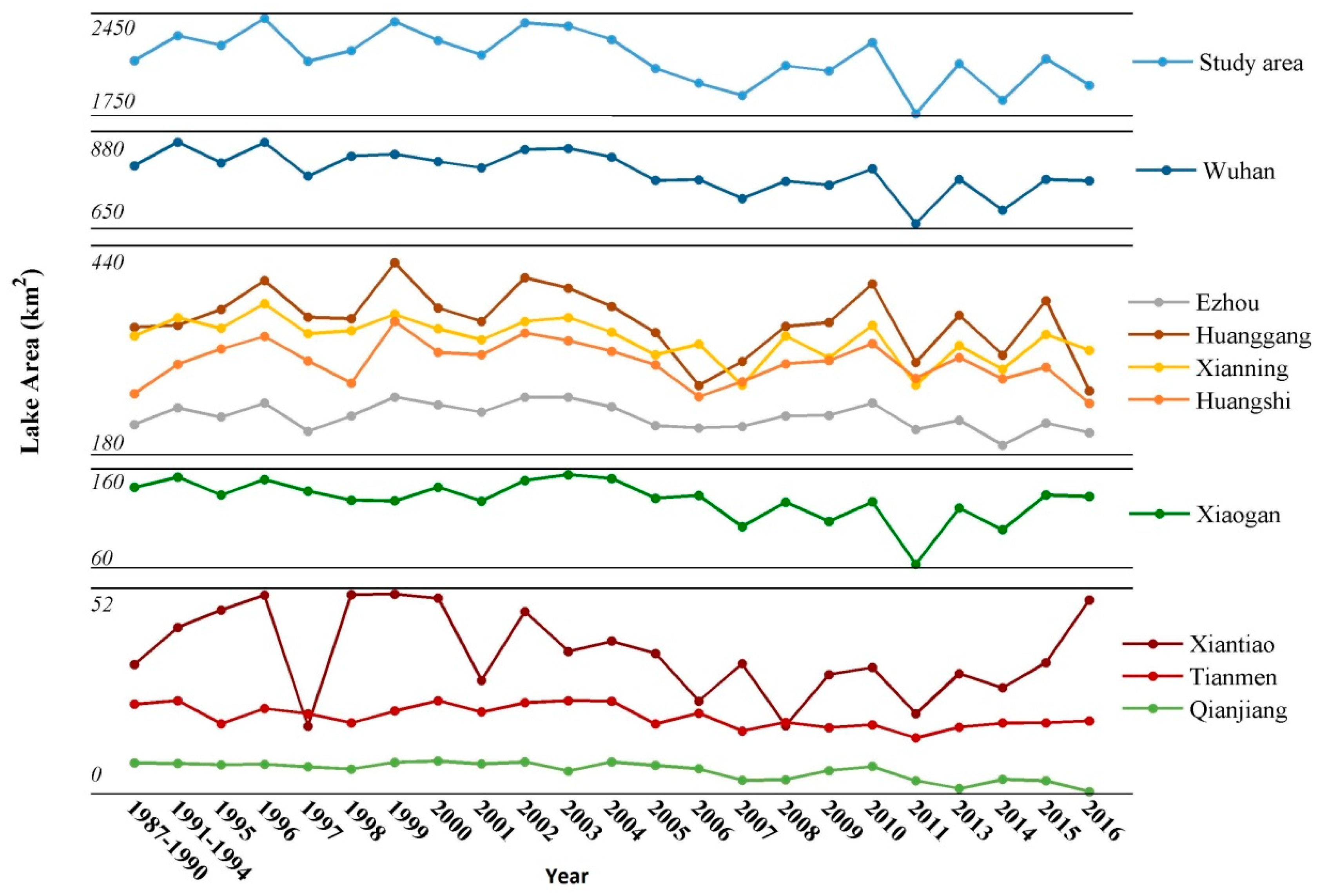
4.4. Lake Water Extent Changes from 1987~2015 in Different Cities
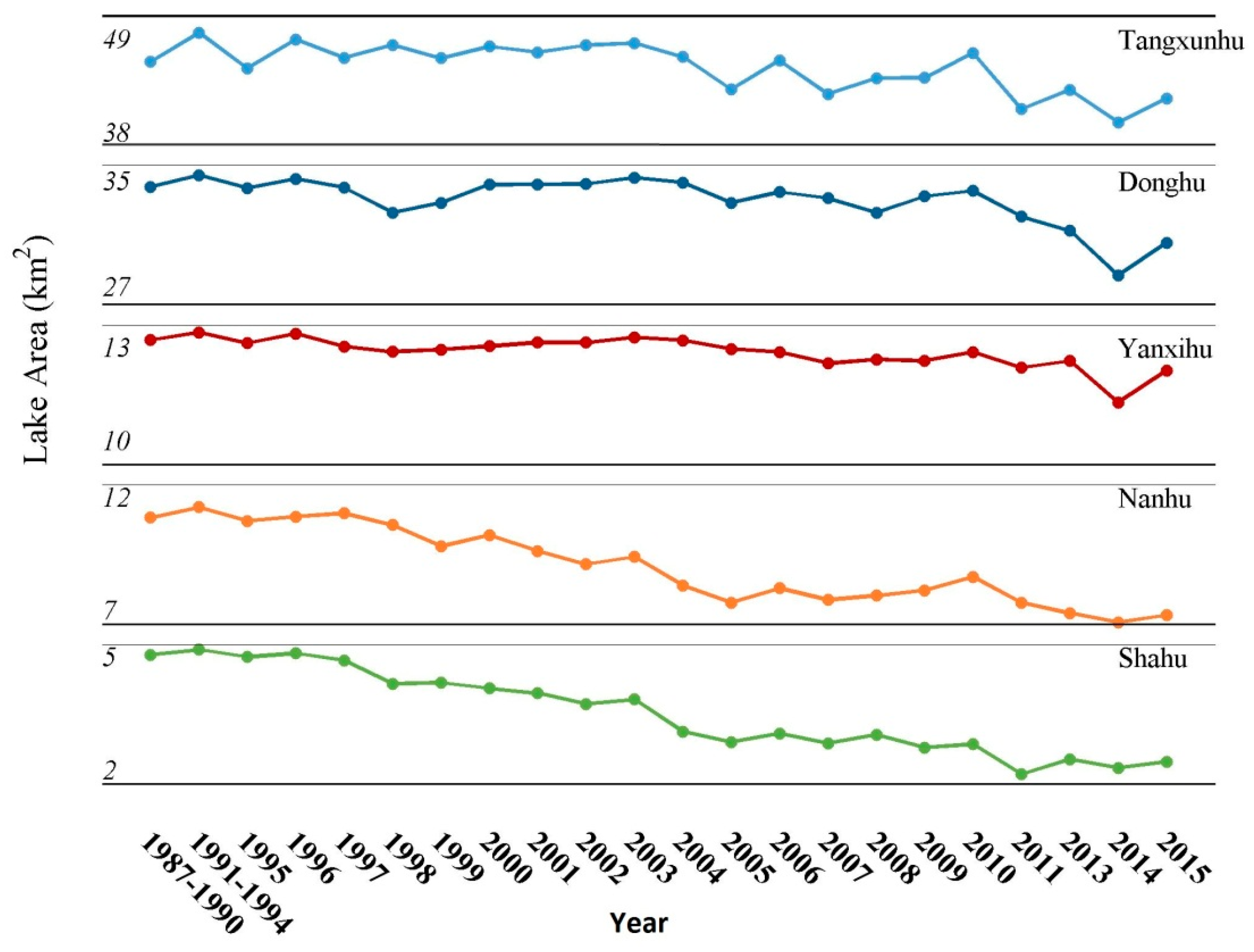
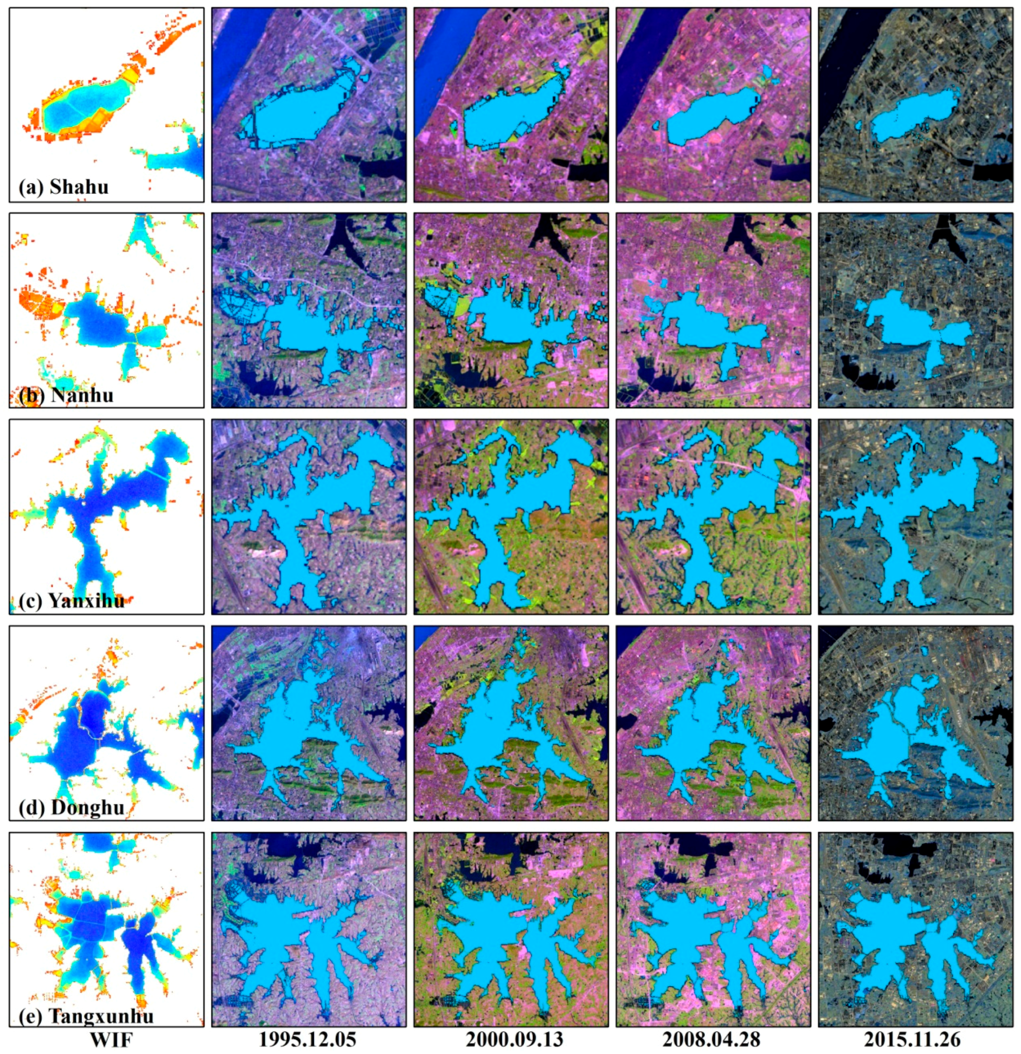
4.5. Decreasing Lake Water Extent Due to Urbanization in Urban Areas
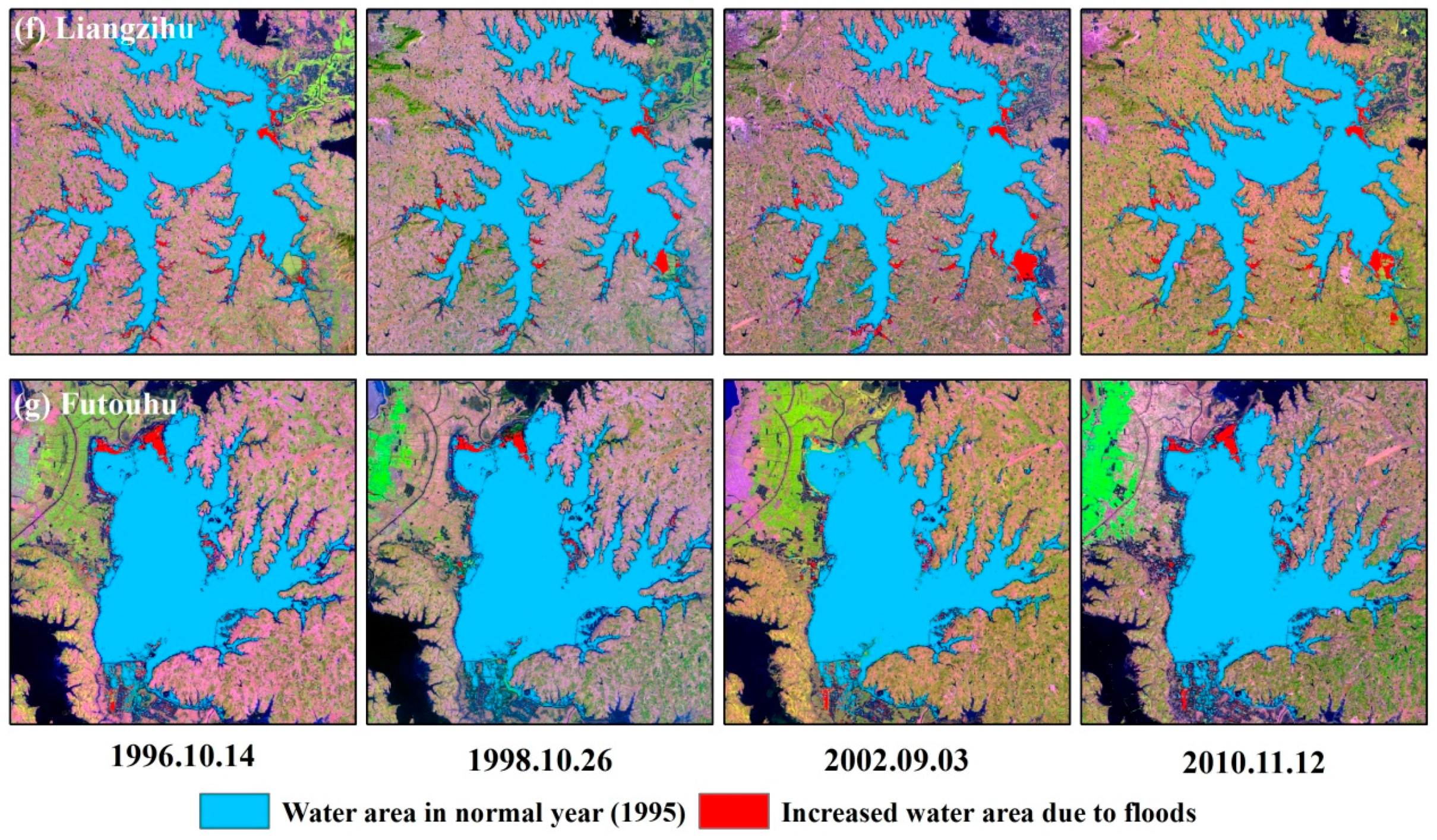
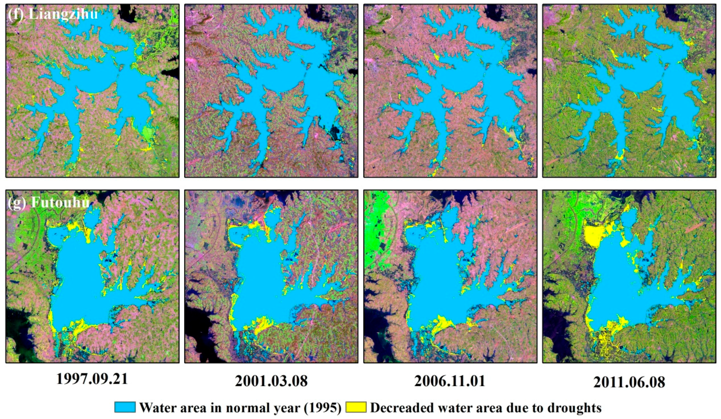
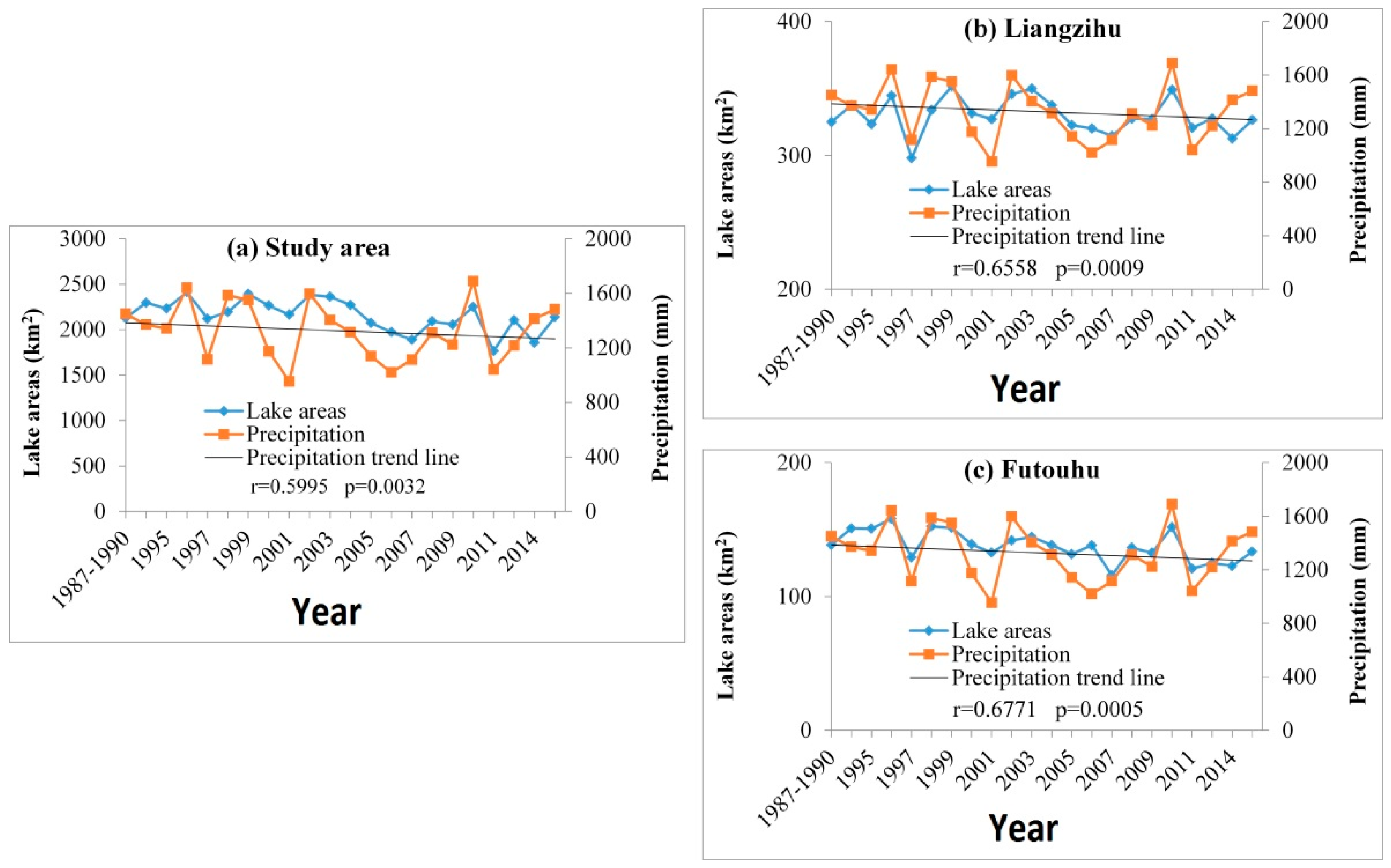
4.6. Lake Water Extent Changes Due to Climate Changes in Non-Urban Areas
5. Discussions
5.1. Long-Term Lake Water Extent Dynamics from Landsat Time Series Data
5.2. Decreasing Lake Water Extent Dynamics Under Urbanization Process and Climate Changes
5.3. Uncertainties and Prospects
6. Conclusions
- (1)
- This study justified the use of the random forest model based on the multi-feature variables to extract water bodies from massive remote-sensing data. Because this method is relatively simple, feasible, and highly accurate, it is a promising method for identifying water bodies at a large scale, such as nationally.
- (2)
- The lake-water areas of the Wuhan urban agglomeration were 226.29 km2, 322.71 km2, 460.35 km2, 400.79 km2, 535.51 km2, and 635.42 km2 under water inundation frequencies of 5%–10%, 10%–20%, 20%–40%, 40%–60%, 60%–80%, and 80%–100%, respectively.
- (3)
- The lake-water area of the Wuhan urban agglomeration experienced a substantial decrease. The area was 2276.03 km2 from 1995–1999, and it decreased to 1966.94 km2 from 2011–2015. In particular, the lake-water areas of loss of Wuhan, Huanggang, Xianning, and Xiaogan were 114.83 km2, 44.40 km2, 45.39 km2, and 31.18 km2, with loss percentages of 14.30%, 11.83%, 13.16%, and 23.05%, respectively.
Acknowledgments
Author Contributions
Conflicts of Interest
References
- Gibbs, J.P. Wetland loss and biodiversity conservation. Conserv. Biol. 2000, 14, 314–317. [Google Scholar] [CrossRef]
- Gleason, R.; Laubhan, M.; Euliss, N. USGS Professional Paper 1745: Ecosystem Services Derived from Wetland Conservation Practices in the United States Prairie Pothole Region with an Emphasis on the U.S. Department of Agriculture Conservation Reserve and Wetlands Reserve Programs. Available online: http://pubs.usgs.gov/pp/1745/ (accessed on 16 October 2016).
- Gabrielsen, C.G.; Murphy, M.A.; Evans, J.S. Using a multiscale, probabilistic approach to identify spatial-temporal wetland gradients. Remote Sens. Environ. 2016, 184, 522–538. [Google Scholar] [CrossRef]
- Yang, B.; Ke, X. Analysis on urban lake change during rapid urbanization using a synergistic approach: A case study of Wuhan, China. Phys. Chem. Earth Parts ABC 2015, 89–90, 127–135. [Google Scholar] [CrossRef]
- Wang, X.; Ning, L.; Yu, J.; Xiao, R.; Li, T. Changes of urban wetland landscape pattern and impacts of urbanization on wetland in Wuhan City. Chin. Geogr. Sci. 2008, 18, 47–53. [Google Scholar] [CrossRef]
- Xu, K.; Kong, C.; Liu, G.; Wu, C.; Deng, H.; Zhang, Y.; Zhuang, Q. Changes of urban wetlands in Wuhan, China, from 1987 to 2005. Prog. Phys. Geogr. 2010, 34, 207–220. [Google Scholar]
- Chen, K.; Wang, X.; Li, D.; Li, Z. Driving force of the morphological change of the urban lake ecosystem: A case study of Wuhan, 1990–2013. Ecol. Model. 2015, 318, 204–209. [Google Scholar] [CrossRef]
- Du, N.; Ottens, H.; Sliuzas, R. Spatial impact of urban expansion on surface water bodies—A case study of Wuhan, China. Landsc. Urban Plan. 2010, 94, 175–185. [Google Scholar] [CrossRef]
- Xu, H.; Bai, Y. Evaluation of urban lake evolution using Google Earth Engine—A case study of Wuhan, China. In Proceedings of the 2015 Fourth International Conference on Agro-Geoinformatics (Agro-geoinformatics), Istanbul, Turkey, 20–24 July 2015; pp. 322–325.
- Elmi, O.; Tourian, M.; Sneeuw, N. Dynamic river masks from multi-temporal satellite imagery: An automatic algorithm using graph cuts optimization. Remote Sens. 2016, 8, 1005. [Google Scholar] [CrossRef]
- Li, L.; Xia, H.; Li, Z.; Zhang, Z. Temporal-spatial evolution analysis of lake size-distribution in the middle and lower Yangtze River Basin using Landsat imagery data. Remote Sens. 2015, 7, 10364–10384. [Google Scholar] [CrossRef]
- Halabisky, M.; Moskal, L.M.; Gillespie, A.; Hannam, M. Reconstructing semi-arid wetland surface water dynamics through spectral mixture analysis of a time series of Landsat satellite images (1984–2011). Remote Sens. Environ. 2016, 177, 171–183. [Google Scholar] [CrossRef]
- Tulbure, M.G.; Broich, M.; Stehman, S.V.; Kommareddy, A. Surface water extent dynamics from three decades of seasonally continuous Landsat time series at subcontinental scale in a semi-arid region. Remote Sens. Environ. 2016, 178, 142–157. [Google Scholar] [CrossRef]
- Mueller, N.; Lewis, A.; Roberts, D.; Ring, S.; Melrose, R.; Sixsmith, J.; Lymburner, L.; McIntyre, A.; Tan, P.; Curnow, S.; Ip, A. Water observations from space: Mapping surface water from 25 years of Landsat imagery across Australia. Remote Sens. Environ. 2016, 174, 341–352. [Google Scholar] [CrossRef]
- Han, X.; Chen, X.; Feng, L. Four decades of winter wetland changes in Poyang Lake based on Landsat observations between 1973 and 2013. Remote Sens. Environ. 2015, 156, 426–437. [Google Scholar] [CrossRef]
- Carroll, M.; Wooten, M.; DiMiceli, C.; Sohlberg, R.; Kelly, M. Quantifying surface water dynamics at 30 meter spatial resolution in the North American high northern latitudes 1991–2011. Remote Sens. 2016, 8, 622. [Google Scholar] [CrossRef]
- Wu, G.; Liu, Y. Mapping Dynamics of inundation patterns of two largest river-connected lakes in China: A comparative study. Remote Sens. 2016, 8, 560. [Google Scholar] [CrossRef]
- Xu, H. Modification of Normalised Difference Water Index (NDWI) to enhance open water features in remotely sensed imagery. Int. J. Remote Sens. 2006, 27, 3025–3033. [Google Scholar] [CrossRef]
- Mcfeeters, S.K. The use of the Normalized Difference Water Index (NDWI) in the delineation of open water features. Int. J. Remote Sens. 1996, 17, 1425–1432. [Google Scholar] [CrossRef]
- Feyisa, G.L.; Meilby, H.; Fensholt, R.; Proud, S.R. Automated water extraction index: A new technique for surface water mapping using Landsat imagery. Remote Sens. Environ. 2014, 140, 23–35. [Google Scholar] [CrossRef]
- Otsu, N. A Threshold selection method from gray-level histograms. IEEE Trans. Syst. Man Cybern. 1979, 9, 62–66. [Google Scholar] [CrossRef]
- Li, W.; Du, Z.; Ling, F.; Zhou, D.; Wang, H.; Gui, Y.; Sun, B.; Zhang, X. A Comparison of land surface water mapping using the normalized difference water index from TM, ETM+ and ALI. Remote Sens. 2013, 5, 5530–5549. [Google Scholar] [CrossRef]
- Rokni, K.; Ahmad, A.; Selamat, A.; Hazini, S. Water feature extraction and change detection using multitemporal Landsat imagery. Remote Sens. 2014, 6, 4173–4189. [Google Scholar] [CrossRef]
- Yang, Y.; Liu, Y.; Zhou, M.; Zhang, S.; Zhan, W.; Sun, C.; Duan, Y. Landsat 8 OLI image based terrestrial water extraction from heterogeneous backgrounds using a reflectance homogenization approach. Remote Sens. Environ. 2015, 171, 14–32. [Google Scholar] [CrossRef]
- Tulbure, M.G.; Broich, M. Spatiotemporal dynamic of surface water bodies using Landsat time-series data from 1999 to 2011. ISPRS J. Photogramm. Remote Sens. 2013, 79, 44–52. [Google Scholar] [CrossRef]
- Gómez, C.; White, J.C.; Wulder, M.A. Optical remotely sensed time series data for land cover classification: A review. ISPRS J. Photogramm. Remote Sens. 2016, 116, 55–72. [Google Scholar] [CrossRef]
- Khatami, R.; Mountrakis, G.; Stehman, S.V. A meta-analysis of remote sensing research on supervised pixel-based land-cover image classification processes: General guidelines for practitioners and future research. Remote Sens. Environ. 2016, 177, 89–100. [Google Scholar] [CrossRef]
- Li, X.; Gong, P.; Liang, L. A 30-year (1984–2013) record of annual urban dynamics of Beijing City derived from Landsat data. Remote Sens. Environ. 2015, 166, 78–90. [Google Scholar] [CrossRef]
- Chander, G.; Markham, B.L.; Helder, D.L. Summary of current radiometric calibration coefficients for Landsat MSS, TM, ETM+, and EO-1 ALI sensors. Remote Sens. Environ. 2009, 113, 893–903. [Google Scholar] [CrossRef]
- Huete, A.; Didan, K.; Miura, T.; Rodriguez, E.P.; Gao, X.; Ferreira, L.G. Overview of the radiometric and biophysical performance of the MODIS vegetation indices. Remote Sens. Environ. 2002, 83, 195–213. [Google Scholar] [CrossRef]
- Tucker, C.J. Red and photographic infrared linear combinations for monitoring vegetation. Remote Sens. Environ. 1979, 8, 127–150. [Google Scholar] [CrossRef]
- Gao, B. NDWI—A normalized difference water index for remote sensing of vegetation liquid water from space. Remote Sens. Environ. 1996, 58, 257–266. [Google Scholar] [CrossRef]
- Tang, Z.; Li, Y.; Gu, Y.; Jiang, W.; Xue, Y.; Hu, Q.; LaGrange, T.; Bishop, A.; Drahota, J.; Li, R. Assessing Nebraska playa wetland inundation status during 1985–2015 using Landsat data and Google Earth Engine. Environ. Monit. Assess. 2016, 188, 654. [Google Scholar] [CrossRef] [PubMed]
- Breiman, L. Random Forests. Mach. Learn. 2001, 45, 5–32. [Google Scholar] [CrossRef]
- Gislason, P.O.; Benediktsson, J.A.; Sveinsson, J.R. Random Forests for Land Cover Classification. Pattern Recogn. Lett. 2006, 27, 294–300. [Google Scholar] [CrossRef]
- Yu, X.; Hyyppä, J.; Vastaranta, M.; Holopainen, M.; Viitala, R. Predicting individual tree attributes from airborne laser point clouds based on the random forests technique. ISPRS J. Photogramm. Remote Sens. 2011, 66, 28–37. [Google Scholar] [CrossRef]
- Stumpf, A.; Kerle, N. Object-oriented mapping of landslides using random forests. Remote Sens. Environ. 2011, 115, 2564–2577. [Google Scholar] [CrossRef]
- Zhu, Z.; Woodcock, C.E. Automated cloud, cloud shadow, and snow detection in multitemporal Landsat data: An algorithm designed specifically for monitoring land cover change. Remote Sens. Environ. 2014, 152, 217–234. [Google Scholar] [CrossRef]


| Sensor | Path/Row | ||||||||
|---|---|---|---|---|---|---|---|---|---|
| 121/39 | 122/38 | 122/39 | 122/40 | 123/38 | 123/39 | 123/40 | 124/39 | Total | |
| TM (1987–2011) | 122 | 130 | 141 | 124 | 139 | 129 | 115 | 119 | 1019 |
| ETM (1999–2003) | 26 | 23 | 23 | 19 | 24 | 22 | 22 | 21 | 180 |
| OLI (2013–2015) | 25 | 22 | 20 | 25 | 26 | 23 | 21 | 14 | 176 |
| Total | 173 | 175 | 184 | 168 | 189 | 175 | 158 | 154 | 1375 |
| Samples | TM | ETM | OLI |
|---|---|---|---|
| water bodies | 46,041 | 63,272 | 54,300 |
| non-water bodies | 521,279 | 172,391 | 189,121 |
| Total | 567,320 | 235,663 | 243,421 |
| Sensor Type | Date | Extracted Lake Area (km2) | True Lake Area (km2) | Accuracy (%) |
|---|---|---|---|---|
| TM | 1995/12/5 | 1003.64 | 1077.24 | 93.17 |
| ETM | 2000/1/11 | 618.19 | 649.76 | 95.14 |
| ETM | 2000/7/22 | 658.91 | 686.08 | 96.04 |
| TM | 2004/2/13 | 828.95 | 903.92 | 91.71 |
| TM | 2004/7/22 | 789.64 | 826.57 | 95.53 |
| TM | 2009/9/9 | 760.88 | 848.40 | 89.68 |
| OLI | 2013/9/17 | 810.32 | 898.67 | 90.17 |
| OLI | 2015/11/26 | 899.70 | 963.17 | 93.41 |
| Lake Name | Lake Area (km2) | Loss Rate (km2/year) | |||||
|---|---|---|---|---|---|---|---|
| 1995 | 2000 | 2008 | 2015 | 1995–2000 | 2000–2008 | 2008–2015 | |
| TangXunHu | 44.52 | 46.40 | 43.70 | 41.98 | −0.38 | 0.34 | 0.25 |
| DongHu | 33.62 | 33.82 | 32.24 | 30.53 | −0.04 | 0.20 | 0.24 |
| YanXiHu | 12.59 | 12.53 | 12.25 | 12.01 | 0.01 | 0.04 | 0.03 |
| NanHu | 10.68 | 10.18 | 8.03 | 7.34 | 0.10 | 0.27 | 0.10 |
| ShaHu | 4.72 | 4.05 | 3.06 | 2.48 | 0.13 | 0.12 | 0.08 |
© 2017 by the authors. Licensee MDPI, Basel, Switzerland. This article is an open access article distributed under the terms and conditions of the Creative Commons Attribution (CC BY) license ( http://creativecommons.org/licenses/by/4.0/).
Share and Cite
Deng, Y.; Jiang, W.; Tang, Z.; Li, J.; Lv, J.; Chen, Z.; Jia, K. Spatio-Temporal Change of Lake Water Extent in Wuhan Urban Agglomeration Based on Landsat Images from 1987 to 2015. Remote Sens. 2017, 9, 270. https://doi.org/10.3390/rs9030270
Deng Y, Jiang W, Tang Z, Li J, Lv J, Chen Z, Jia K. Spatio-Temporal Change of Lake Water Extent in Wuhan Urban Agglomeration Based on Landsat Images from 1987 to 2015. Remote Sensing. 2017; 9(3):270. https://doi.org/10.3390/rs9030270
Chicago/Turabian StyleDeng, Yue, Weiguo Jiang, Zhenghong Tang, Jiahong Li, Jinxia Lv, Zheng Chen, and Kai Jia. 2017. "Spatio-Temporal Change of Lake Water Extent in Wuhan Urban Agglomeration Based on Landsat Images from 1987 to 2015" Remote Sensing 9, no. 3: 270. https://doi.org/10.3390/rs9030270
APA StyleDeng, Y., Jiang, W., Tang, Z., Li, J., Lv, J., Chen, Z., & Jia, K. (2017). Spatio-Temporal Change of Lake Water Extent in Wuhan Urban Agglomeration Based on Landsat Images from 1987 to 2015. Remote Sensing, 9(3), 270. https://doi.org/10.3390/rs9030270