Predictions of Tropical Forest Biomass and Biomass Growth Based on Stand Height or Canopy Area Are Improved by Landsat-Scale Phenology across Puerto Rico and the U.S. Virgin Islands


Abstract
:
1. Introduction
- AB: aboveground biomass
- BB: belowground biomass
- DW: deadwood
- LI: litter
- SO: soils
- HWP: harvested wood products.
2. Materials and Methods
2.1. Study Area
2.2. Methods
2.2.1. Field Data Collection and Processing
- t1 = Julian day of the first survey in fractional y
- t2 = Julian day of the second survey in fractional y
- tm = Julian day of the midpoint between the first and second surveys in fractional y
- t2 − t1 = Interval between the first and second survey dates in fractional y
- NBG = Net Biomass Growth at the plot level, in Mg·ha−1·y−1, from t1 to t2
- SABtx = Biomass of survivor tree i estimated for tx, as indicated
- IABtx = Biomass of ingrowth tree i estimated for tx, as indicated
- MABtx = Biomass of mortality tree i estimated for tx, as indicated
- S = The number of trees that survived from t1 to t2
- I = The number of trees in micro-plots that reached a dbh of 12.7 cm in t2
- M = The number of trees that died in the interval from t1 to t2
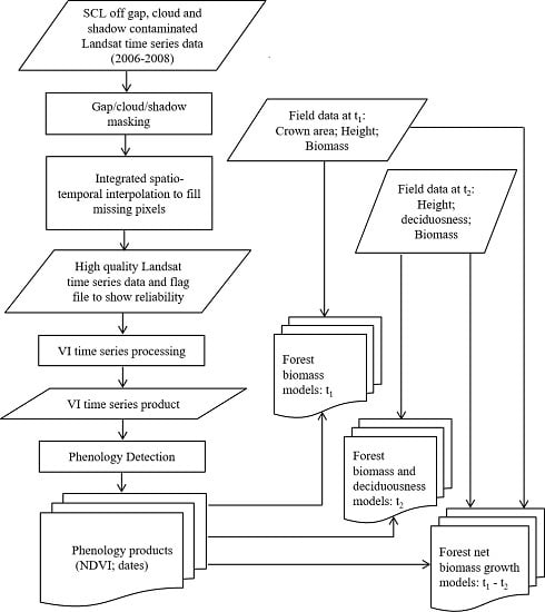
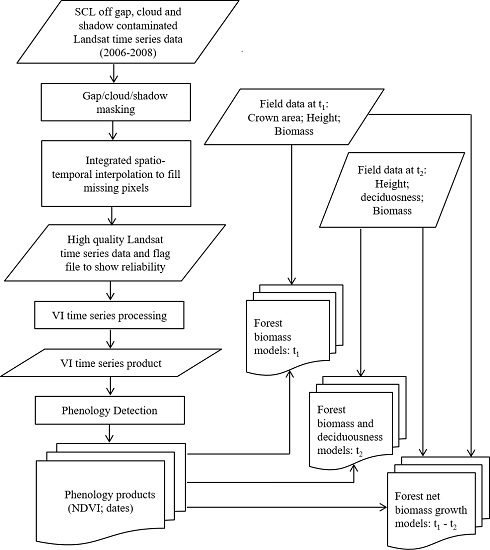
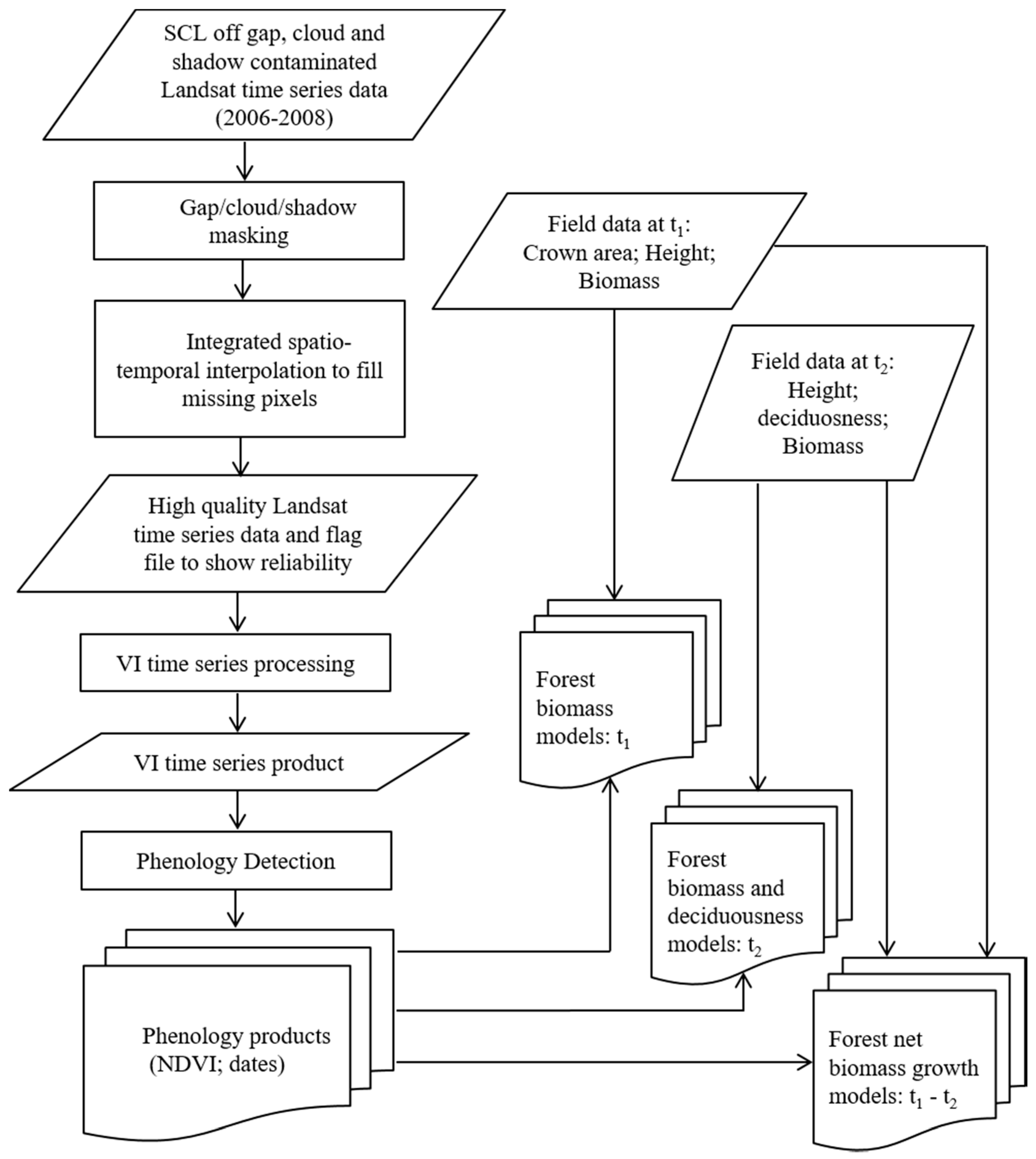
2.2.2. Phenology Detection
2.3. Statistical Analysis
3. Results
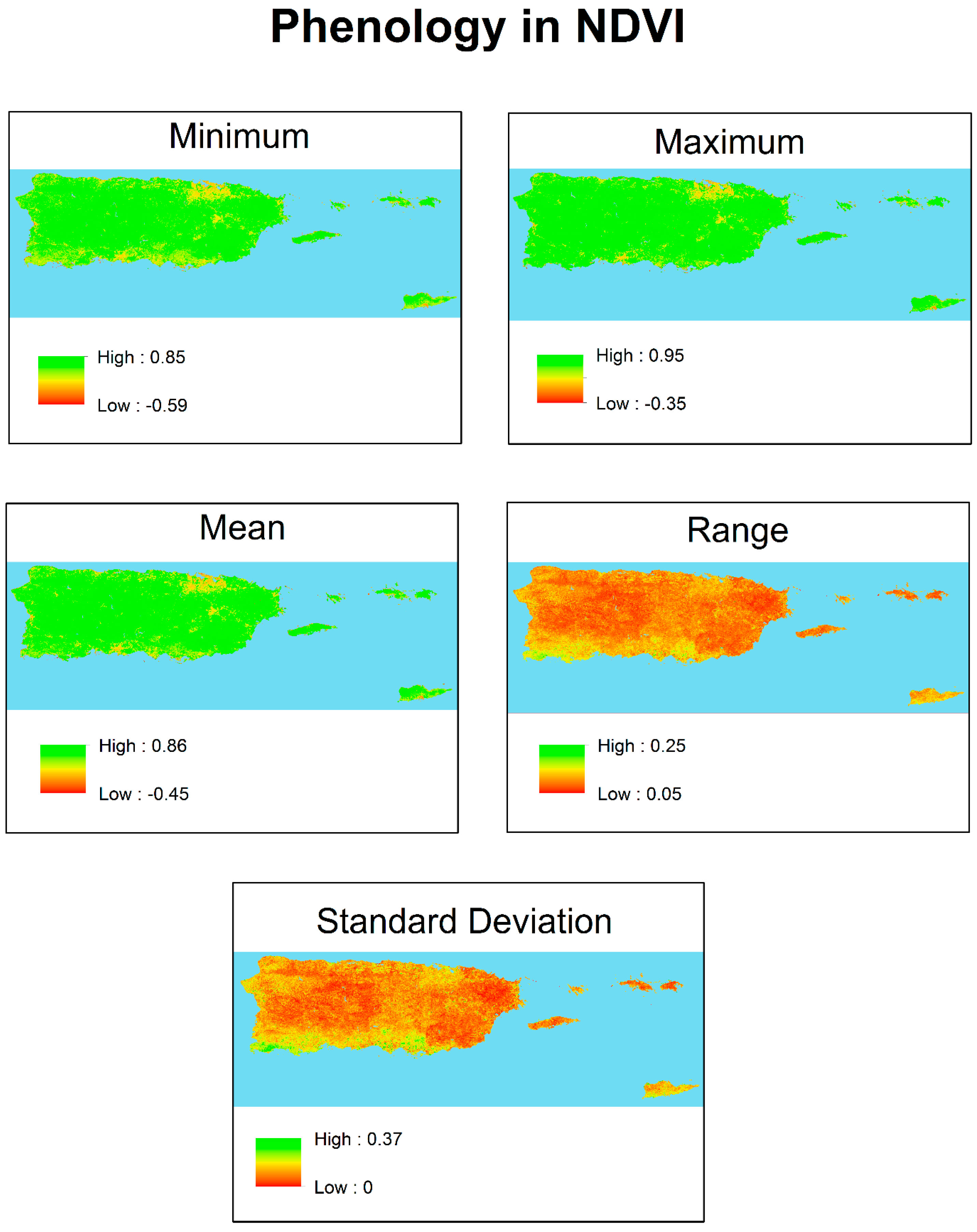
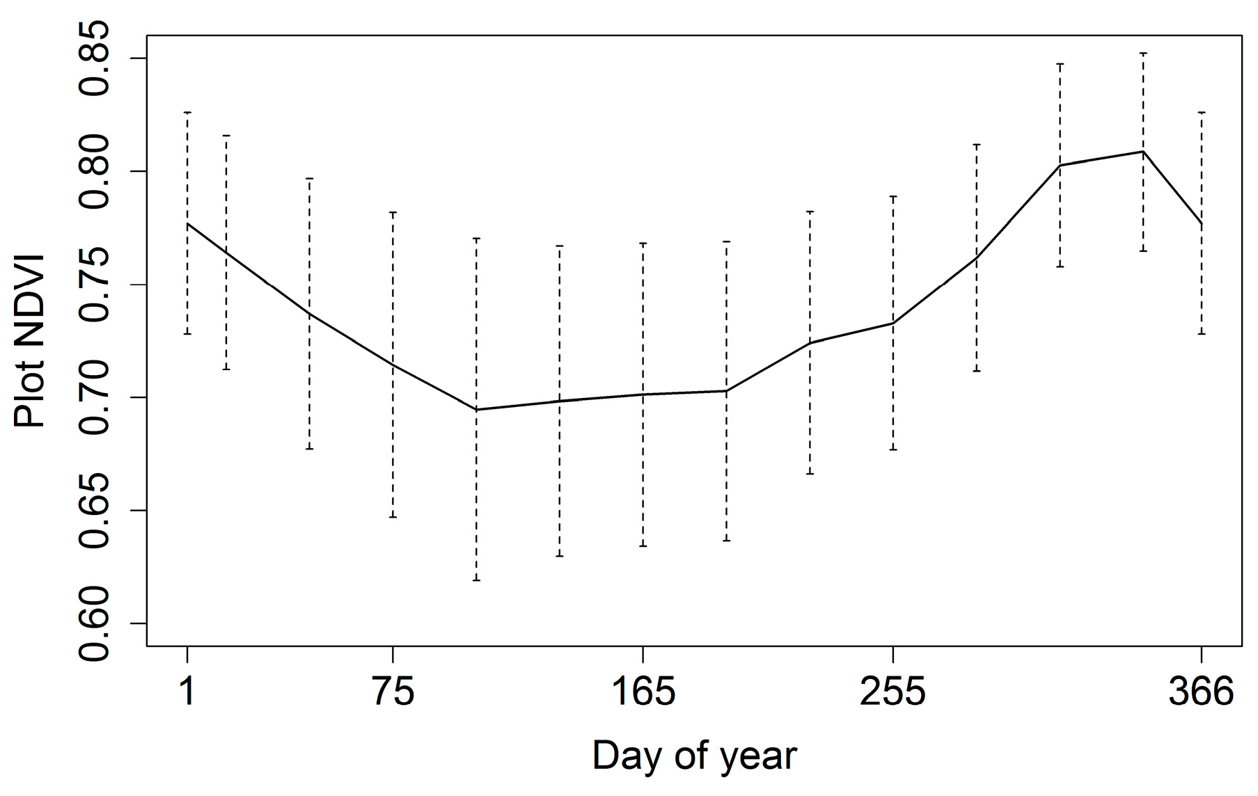
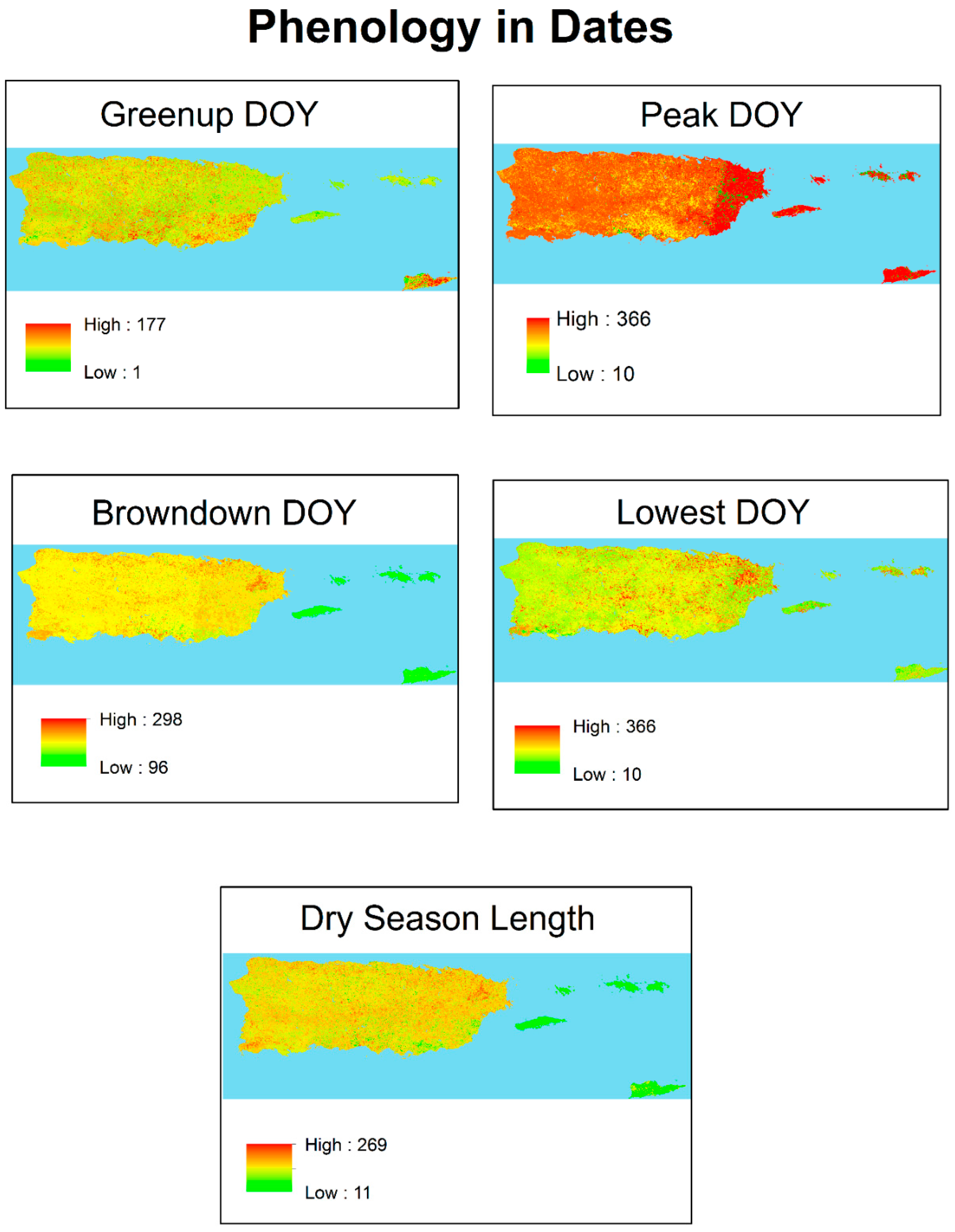
3.1. Phenology
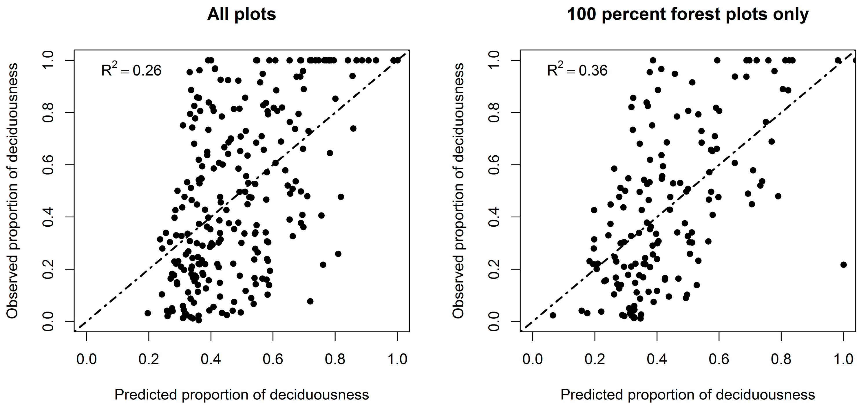
3.2. Forest Deciduousness
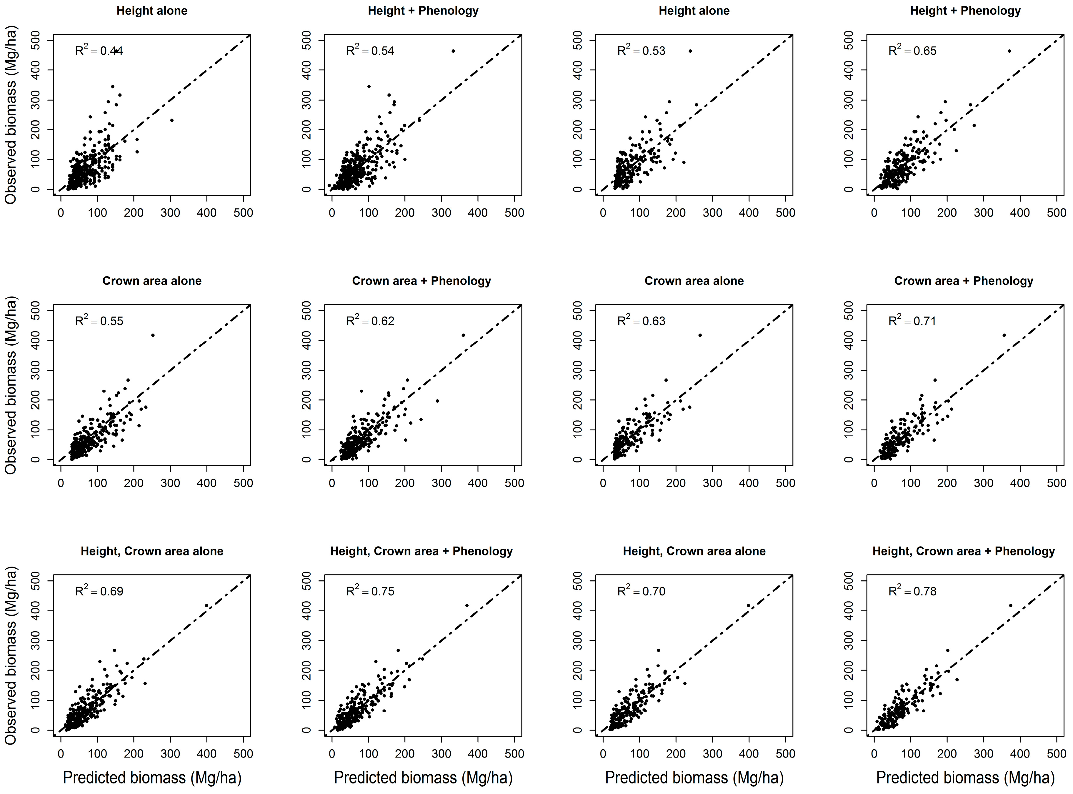
3.3. Forest Biomass
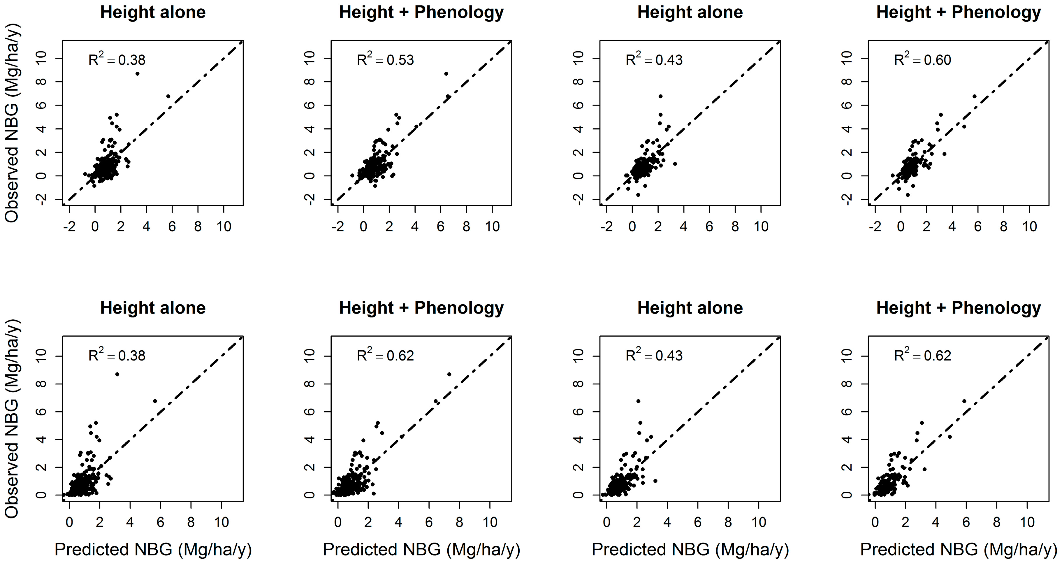
3.4. Forest Net Biomass Growth
4. Discussion
5. Conclusions
Acknowledgments
Author Contributions
Conflicts of Interest
References
- Helmer, E.H.; Goodwin, N.R.; Gond, V.; de Souza, C.M.J.; Asner, G.P. Characterizing tropical forests with multispectral imagery. In Land Resources Monitoring, Modeling and Mapping with Remote Sensing; Thenkabail, P.S., Ed.; Taylor: Boca Raton, FL, USA, 2015; pp. 363–391. [Google Scholar]
- Intergovernmental Panel on Climate Change. 2006 IPCC Guidelines for National Greenhouse Gas Inventories; Prepared by the National Greenhouse Gas Inventories Programme; Eggleston, H.S., Buendia, L., Miwa, K., Ngara, T., Tanabe, K., Eds.; Institute for Global Environmental Strategies (IGES): Kanagawa, Japan, 2006; Volume 4. [Google Scholar]
- Brown, S. Estimating Biomass and Biomass Change of Tropical Forests: A Primer; Food and Agriculture Organization of the United Nations: Rome, Italy, 1997; Volume 134. [Google Scholar]
- Couteron, P.; Pelissier, R.; Nicolini, E.A.; Paget, D. Predicting tropical forest stand structure parameters from Fourier transform of very high-resolution remotely sensed canopy images. J. Appl. Ecol. 2005, 42, 1121–1128. [Google Scholar] [CrossRef]
- Ota, T.; Kajisa, T.; Mizoue, N.; Yoshida, S.; Takao, G.; Hirata, Y.; Furuya, N.; Sano, T.; Ponce-Hernandez, R.; Ahmed, O.S.; et al. Estimating aboveground carbon using airborne LiDAR in Cambodian tropical seasonal forests for REDD+ implementation. J. For. Res. 2015, 20, 484–492. [Google Scholar] [CrossRef]
- Messinger, M.; Asner, G.P.; Silman, M. Rapid assessments of amazon forest structure and biomass using small unmanned aerial systems. Remote Sens. 2016, 8, 615. [Google Scholar] [CrossRef]
- Deo, R.; Russell, M.; Domke, G. Using Landsat Time-series and LiDAR to Inform Aboveground Forest Biomass Baselines in Northern Minnesota, USA. Can. J. Remote Sens. 2016, 43, 28–47. [Google Scholar] [CrossRef]
- Reich, P.B. Phenology of tropical forests: Patterns, causes, and consequences. Can. J. Bot. 1995, 73, 164–174. [Google Scholar] [CrossRef]
- Condit, R.; Watts, K.; Bohlman, S.A.; Pérez, R.; Foster, R.B.; Hubbell, S.P. Quantifying the deciduousness of tropical forest canopies under varying climates. J. Veg. Sci. 2000, 11, 649–658. [Google Scholar] [CrossRef]
- Feldpausch, T.R.; Banin, L.; Phillips, O.L.; Baker, T.R.; Lewis, S.L.; Quesada, C.A.; Affum-Baffoe, K.; Arets, E.J.M.M.; Berry, N.J.; Bird, M.; et al. Height-diameter allometry of tropical forest trees. Biogeosciences 2011, 8, 1081–1106. [Google Scholar] [CrossRef]
- Richardson, A.D.; Braswell, B.H.; Hollinger, D.Y.; Jenkins, J.P.; Richardson, A.D.; Braswell, B.H.; Hollinger, D.Y.; Jenkins, J.P.; Ollinger, S.V. Near-Surface Remote Sensing of Spatial and Temporal Variation in Canopy Phenology. Ecol. Appl. 2009, 19, 1417–1428. [Google Scholar] [CrossRef] [PubMed]
- Hanes, J. Biophysical Applications of Satellite Remote Sensing; Springer: Berlin, Germany, 2014. [Google Scholar]
- Yang, X.; Tang, J.; Mustard, J.F.; Lee, J.; Rossini, M.; Joiner, J.; Munger, J.W.; Kornfeld, A.; Richardson, D.A. Solar-induced chlorophyll fluorescence that correlates with canopy photosynthesis on diurnal and seasonal scales in a temperate deciduous forest. Geophys. Res. Lett. 2015, 42, 2977–2987. [Google Scholar] [CrossRef]
- Zhang, X.; Friedl, M.A.; Schaaf, C.B.; Strahler, A.H.; Hodges, J.C.F.; Gao, F.; Reed, B.C.; Huete, A. Monitoring vegetation phenology using MODIS. Remote Sens. Environ. 2003, 84, 471–475. [Google Scholar] [CrossRef]
- Joiner, J.; Yoshida, Y.; Vasilkov, A.P.; Schaefer, K.; Jung, M.; Guanter, L.; Zhang, Y.; Garrity, S.; Middleton, E.M.; Huemmrich, K.F.; et al. The seasonal cycle of satellite chlorophyll fluorescence observations and its relationship to vegetation phenology and ecosystem atmosphere carbon exchange. Remote Sens. Environ. 2014, 152, 375–391. [Google Scholar] [CrossRef]
- White, M.A.; Thornton, P.E.; Running, S.W. A continental phenology model for monitoring vegetation responses to interannual climatic variability. Global Biogeochem. Cy. 1997, 11, 217–234. [Google Scholar] [CrossRef]
- Zhang, X.; Tarpley, D.; Sullivan, J.T. Diverse responses of vegetation phenology to a warming climate. Geophys. Res. Lett. 2007, 34. [Google Scholar] [CrossRef]
- Guanter, L.; Zhang, Y.; Jung, M.; Joiner, J.; Voigt, M.; Berry, J.A.; Frankenberg, C.; Huete, A.R.; Zarco-Tejada, P.; Lee, J.-E.; et al. Global and time-resolved monitoring of crop photosynthesis with chlorophyll fluorescence. Proc. Natl. Acad. Sci. USA 2014, 111, E1327–E1333. [Google Scholar] [CrossRef] [PubMed]
- Reed, B.C.; Brown, J.F.; VanderZee, D.; Loveland, T.R.; Merchant, J.W.; Ohlen, D.O. Measuring Phenological Variability from Satellite Imagery. J. Veg. Sci. 1994, 5, 703–714. [Google Scholar] [CrossRef]
- Helmer, E.H.; Ruefenacht, B. A comparison of radiometric normalization methods when filling cloud gaps in Landsat imagery. Can. J. Remote Sens. 2007, 33, 325–340. [Google Scholar] [CrossRef]
- Helmer, E.H.; Ruzycki, T.S.; Benner, J.; Voggesser, S.M.; Scobie, B.P.; Park, C.; Fanning, D.W.; Ramnarine, S. Detailed maps of tropical forest types are within reach: Forest tree communities for Trinidad and Tobago mapped with multiseason Landsat and multiseason fine-resolution imagery. For. Ecol. Manag. 2012, 279, 147–166. [Google Scholar] [CrossRef]
- Zhu, X.; Helmer, E.; Lefsky, M.A. An automated method to mask cloud and cloud shadow in optical time-series images. 2017; pending preparation. [Google Scholar]
- Zhu, X.; Helmer, E.; Gwenzi, D.; Lefsky, M.A. Reconstructing seasonal Landsat time-series to detect tropical forest phenology in Mona Island, Puerto Rico. In Proceeding of the AGU Annual Meeting, San Francisco, CA, USA, 12–16 December 2016.
- Brandeis, T.J.; Helmer, E.H.; Marcano-Vega, H.; Lugo, A.E. Climate shapes the novel plant communities that form after deforestation in Puerto Rico and the U.S. Virgin Islands. For. Ecol. Manag. 2009, 258, 1704–1718. [Google Scholar] [CrossRef]
- Daly, C.; Helmer, E.H.; Quinones, M. Mapping the climate of Puerto Rico, Vieques and Culebra. Int. J. Climatol. 2003, 23, 1359–1381. [Google Scholar] [CrossRef]
- Helmer, E.H.; Ramos, O.; López, T.D.M.; Quiñones, M.; Díaz, W. Mapping the forest type and land cover of Puerto Rico, a component of the Caribbean biodiversity hotspot. Caribb. J. Sci. 2002, 38, 165–183. [Google Scholar]
- Bechtold, W.A.; Patterson, P.L. The Enhanced Forest Inventory and Analysis Program—National Sampling Design and Estimation Procedures; Gen. Tech. Rep. SRS-80; U.S. Department of Agriculture, Forest Service, Southern Research Station: Ashville, NC, USA, 2005.
- Ju, J.; Roy, D.P. The availability of cloud-free Landsat ETM+ data over the conterminous United States and globally. Remote Sens. Environ. 2008, 112, 1196–1211. [Google Scholar] [CrossRef]
- Holdridge, L.R. Life Zone Ecology; Tropical Science Center: San Jose, Costa Rica, 1967. [Google Scholar]
- Frangi, J.L.; Lugo, A.E. Ecosystem Dynamics of a Subtropical Floodplain Forest. Ecol. Monogr. 1985, 55, 351–369. [Google Scholar] [CrossRef]
- Weaver, P.L.; Gillespie, A.J.R. Tree Biomass Equations for the Forests of the Luquillo Mountains, Puerto Rico. Commonw. For. Rev. 1992, 71, 35–39. [Google Scholar]
- Scatena, A.F.N.; Silver, W.; Siccama, T.; Johnson, A.; Sanchez, M.J. Biomass and Nutrient Content of the Bisley Experimental Watersheds, Luquillo Experimental Forest, Puerto Rico, Before and After Hurricane Hugo, 1989. Biotropica 1993, 25, 15–27. [Google Scholar] [CrossRef]
- Brandeis, T.J.; Delaney, M.; Parresol, B.R.; Royer, L. Development of equations for predicting Puerto Rican subtropical dry forest biomass and volume. For. Ecol. Manag. 2006, 233, 133–142. [Google Scholar] [CrossRef]
- Brandeis, T.J.; Helmer, E.H.; Oswalt, S.N. The Status of Puerto Rico’s Forests, 2003; U.S. Department of Agriculture, Forest Service, Southern Research Station: Asheville, NC, USA, 2007.
- Brandeis, T.J.; Oswalt, S.N. The Status of U.S. Virgin Islands’ Forests, 2004; U.S. Department of Agriculture, Forest Service, Southern Research Station: Asheville, NC, USA, 2007.
- Palace, M.W.; Sullivan, F.B.; Ducey, M.J.; Treuhaft, R.N.; Herrick, C.; Shimbo, J.Z.; Mota-E-Silva, J. Estimating forest structure in a tropical forest using field measurements, a synthetic model and discrete return lidar data. Remote Sens. Environ. 2015, 161, 1–11. [Google Scholar] [CrossRef]
- Irish, R.R.; Barker, J.L.; Goward, T.A. Characterization of the Landsat-7 ETM+ automated cloud-cover assessment (ACCA) algorithm. Photogramm. Eng. Remote Sens. 2006, 72, 1179–1188. [Google Scholar] [CrossRef]
- Huang, C.; Thomas, N.; Goward, S.N.; Masek, J.G.; Zhu, Z.; Townsend, J.R.; Vogelmann, J.E. Automated masking of cloud and cloud shadow for forest change analysis using Landsat images. Int. J. Remote Sens. 2010, 31, 5449–5464. [Google Scholar] [CrossRef]
- Roy, D.P.; Ju, J.; Kline, K.; Scaramuzza, P.L.; Kovalskyy, V.; Hansen, M.; Loveland, T.R.; Vermote, E.; Zhang, C. Web-enabled Landsat Data (WELD): Landsat ETM+ composited mosaics of the conterminous United States. Remote Sens. Environ. 2010, 114, 35–49. [Google Scholar] [CrossRef]
- Zhu, Z.; Woodcock, C.E. Object-based cloud and cloud shadow detection in Landsat imagery. Remote Sens. Environ. 2012, 118, 83–94. [Google Scholar] [CrossRef]
- Zhu, Z.; Wang, S.; Woodcock, C.E. Improvement and expansion of the Fmask algorithm: Cloud, cloud shadow, and snow detection for Landsats 4-7, 8, and Sentinel 2 images. Remote Sens. Environ. 2015, 159, 269–277. [Google Scholar] [CrossRef]
- Zhu, X.; Gao, F.; Liu, D.; Chen, J. A modified neighborhood similar pixel interpolator approach for removing thick clouds in landsat images. IEEE Geosci. Remote Sens. Lett. 2012, 9, 521–525. [Google Scholar] [CrossRef]
- Chen, J.; Zhu, X.; Vogelmann, J.E.; Gao, F.; Jin, S. A simple and effective method for filling gaps in Landsat ETM+ SLC-off images. Remote Sens. Environ. 2011, 115, 1053–1064. [Google Scholar] [CrossRef]
- Chen, J.; Rao, Y.; Shen, M.; Wang, C.; Zhou, Y.; Ma, L.; Tang, Y.; Yang, X. A Simple Method for Detecting Phenological Change From Time Series of Vegetation Index. IEEE Trans. Geosci. Remote Sens. 2016, 54, 3436–3449. [Google Scholar] [CrossRef]
- Chen, J.; Jonsson, P.; Tamura, M.; Gu, Z.; Matsushita, B.; Eklundh, L. A simple method for reconstructing a high-quality NDVI time-series data set based on the Savitzky-Golay filter. Remote Sens. Environ. 2004, 91, 332–344. [Google Scholar] [CrossRef]
- Savitzky, A.; Golay, M.J.E. Smoothing and Differentiation of Data by Simplified Least Squares Procedures. Anal. Chem. 1964, 36, 1627–1639. [Google Scholar] [CrossRef]
- Anderson, L.O.; Malhi, Y.; Aragão, L.E.O.C.; Ladle, R.; Arai, E.; Barbier, N.; Phillips, O. Remote sensing detection of droughts in Amazonian forest canopies. New Phytol. 2010, 187, 733–750. [Google Scholar] [CrossRef] [PubMed]
- Zalamea, M.; Gonzalez, G. Leaffall phenology in a subtropical wet forest in Puerto Rico: From species to community patterns. Biotropica 2008, 40, 295–304. [Google Scholar] [CrossRef]
- Martínez, O.J.A. Flooding and profuse flowering result in high litterfall in novel Spathodea campanulata forests in northern Puerto Rico. Ecosphere 2011, 2, art105. [Google Scholar] [CrossRef]
- Brandeis, T.J.; Turner, J.A. Puerto Rico’s Forests, 2009; U.S. Department of Agriculture, Forest Service, Southern Research Station: Asheville, NC, USA, 2013.
- Van Schaik, C.P.; Terborgh, J.W.; Wright, S.J. The Phenology of Tropical Forests: Adaptive Significance and Consequences for Primary Consumers. Annu. Rev. Ecol. Syst. 1993, 24, 353–377. [Google Scholar] [CrossRef]
- Boyle, A.W.; Bronstein, J.L. Phenology of tropical understory trees: Patterns and correlates. Rev. Biol. Trop. 2012, 60, 1415–1429. [Google Scholar] [CrossRef] [PubMed]
- Fan, H.; Fu, X.; Zhang, Z.; Wu, Q. Phenology-based vegetation index differencing for mapping of rubber plantations using landsat OLI data. Remote Sens. 2015, 7, 6041–6058. [Google Scholar] [CrossRef]
- Reich, P.B. Key canopy traits drive forest productivity. Proc. R. Soc. B-Biol. Sci. 2012, 279, 2128–2134. [Google Scholar] [CrossRef] [PubMed]
- Zhang, X.; Friedl, M.A.; Schaaf, C.B. Sensitivity of vegetation phenology detection to the temporal resolution of satellite data. Int. J. Remote Sens. 2009, 30, 2061–2074. [Google Scholar] [CrossRef]


| Year | Landsat Scene: Path/Row Number Combination and Image Date (Julian Day of Year) | |||
|---|---|---|---|---|
| 4/47 | 4/48 | 5/47 | 5/48 | |
| 2006 | 39; 55; 71; 167; 183; 263; 311 | 23; 55; 71; 119; 135; 167; 183; 263;311 | 09; 78; 94; 110; 126; 286; 350 | 14; 46; 78; 94; 110; 126; 142; 286; 318; 350 |
| 2007 | 10; 26; 42; 74; 106; 122; 218; 266 | 10; 26; 42; 74; 170; 186; 202 | 49; 209; 225 | 17; 49; 145; 209; 225; 273; 305; 337; 353 |
| 2008 | 45; 61; 77; 109; 125; 141; 221; 237; 269 | 45; 61; 71; 109; 125; 141; 221 | 100; 132; 276; 292; 308; 340; 356 | 36; 68; 100; 132; 292; 308; 324; 340; 356 |
| NDVI | ||||
| Minimum | Maximum | Mean | Range | Standard Deviation |
| 0.64 | 0.80 | 0.72 | 0.15 | 0.05 |
| Julian Day of Year | ||||
| Peak | Lowest | Greenup | Browndown | Dry Season Length |
| 339 | 126 | 203 | 65 | 137 days |
| Model | Significant Variables at α = 0.05 Level | Adj. R2 | Additional Variation Explained by Phenology | Significant Variables at α = 0.05 Level | Adj. R2 | Additional Variation Explained by Phenology |
|---|---|---|---|---|---|---|
| Modeling Biomass at t2 Using Height and Phenology | ||||||
| All Plots, n = 301 | 100% Forest Plots Only, n = 211 | |||||
| Hdomcod alone | Ht2 | 0.43 | 11% | Ht2 | 0.53 | 12% |
| Hdomcod + phenology | Ht2; ndvi_mean; lowest; greenup; Ht*lowest; Ht2*ndvi_mean; Ht2*lowest; Ht2*greenup | 0.54 | Ht2; lowest; dsl; Ht*ndvi_std; Ht*lowest; Ht2*ndvi_std; Ht2 *lowest | 0.65 | ||
| Hmax alone | Ht2 | 0.44 | 5% | Ht | 0.45 | 6% |
| Hmax + phenology | Ht2; ndvi_min; lowest; greenup; Ht2*peak | 0.49 | Ht; lowest; greenup; Ht*lowest | 0.51 | ||
| Modeling Biomass at t1; Using Crown Area and Phenology (No Height) | ||||||
| All Plots, n = 248 | 100% Forest Plots Only, n = 164 | |||||
| Crown area alone | Carea + carea2 | 0.55 | 7% | Carea + carea2 | 0.63 | 8% |
| Crown area + phenology | carea; carea2; greenup; carea*greenup; carea2*lowest; carea2*greenup | 0.62 | carea; peak; carea*ndvi_max; carea*lowest; carea2*lowest | 0.71 | ||
| Modeling Biomass at t1; Using Height; Crown Area and Phenology | ||||||
| All Plots, n = 248 | 100% Forest Plots Only, n = 164 | |||||
| Hcawgt + crown area | Carea; Ht2; Ht2*carea | 0.67 | 6% | Carea; Ht*carea; Ht | 0.68 | 8% |
| Hcawgt + crown area + phenology | Carea; Ht2*carea; Ht2; carea2*lowest; lowest; dsl; carea*lowest; Ht2*dsl | 0.73 | Ht; lowest; carea2*lowest; dsl; carea; Ht*ndvi_max; Ht*carea; carea*lowest; Ht*dsl | 0.76 | ||
| Hdomcod + crown area | Carea; Ht2*carea2; Ht2 | 0.68 | 7% | Ht*carea2; carea; Ht; Ht2 | 0.69 | 9% |
| Hdomcod + crown area + phenology | Carea; Ht*ndvi_std; dsl; Ht2*carea; Ht*ndvi_std; carea2*lowest; Ht*dsl; carea2*ndvi_min; lowest; carea2; carea*lowest; min | 0.75 | Ht; Ht2*ndvi_max; greenup; Ht*carea2; Ht2; lowest; carea; Ht*greenup; carea2*lowest; ndvi_max | 0.78 | ||
| Hmax + Crown area | Carea; carea2; Ht*carea2 | 0.69 | 6% | carea; carea2; Ht*carea2 | 0.70 | 7% |
| Hmax + crown area + phenology | Carea; Ht2*peak; Ht*peak; Ht; greenup; carea2; Ht2 | 0.75 | carea; Ht2*carea; Ht; dsl; Ht*ndvi_max; Ht2; lowest; Ht*dsl | 0.77 | ||
| Model | Significant Variables at α = 0.05 Level | Adj. R2 | Additional Variation Explained by Phenology | Significant Variables at α = 0.05 Level | Adj. R2 | Additional Variation Explained by Phenology |
|---|---|---|---|---|---|---|
| All Plots, n = 261 | All 100% Forest Plots, n = 170 | |||||
| Hdomcod alone | Ht2 | 0.27 | 16% | Ht2 | 0.35 | 21% |
| Hdomcod + phenology | Ht2*ndvi_std; peak; Ht2*peak; greenup; ndvi_std; Ht2*ndvi_min; Ht*ndvi_std; Ht2*ndvi_mean; Ht2; ndvi_min; Ht2*greenup | 0.43 | Peak; Ht2*ndvi_std; ndvi_std; Ht2; greenup; ndvi_mean; Ht*ndvi_mean; Ht*peak | 0.56 | ||
| Hdomcod + ΔHdomcod | Ht2; ΔHt | 0.34 | 19% | Ht2, ΔHt | 0.43 | 17% |
| Hdomcod + ΔHdomcod + phenology | ΔHt*peak; ΔHt; Ht2*ndvi_std; Ht2*ndvi_min; Ht2; ΔHt*ndvi_mean; Ht*std; ΔHt*ndvi_min | 0.53 | ΔHt; Ht2; Ht2*ndvi_std; ndvi_std; ΔHt*peak; Ht*ndvi_std | 0.60 | ||
| Hmax alone | Ht, Ht2 | 0.29 | 11% | Ht, Ht2 | 0.37 | 12% |
| Hmax + phenology | Ht2; Ht2*peak; Ht2*ndvi_std; Ht2*ndvi_range, peak; ndvi_std; ndvi_range | 0.40 | Ht2; greenup; Ht2*greenup; ndvi_std; Ht2*ndvi_std; Ht*ndvi_std; Ht | 0.49 | ||
| Hmax + ΔHmax | Ht2; ΔHt | 0.38 | 12% | Ht2, ΔHt | 0.42 | 11% |
| Hmax + ΔHmax + phenology | ΔHt; Ht2*ndvi_std; ΔHt*ndvi_max; Ht2*peak; Ht*ndvi_range; Ht2; peak; ndvi_std | 0.50 | Ht2*ndvi_std; Ht*ndvi_range; ΔHt; Ht2; ndvi_std; peak; Ht*peak | 0.53 | ||
| All Plots with Positive Growth Only, n = 244 | 100% Forest Plots with Positive Growth Only, n = 161 | |||||
| Hdomcod alone | Ht2 | 0.30 | 17% | Ht2 | 0.40 | 22% |
| Hdomcod + phenology | Ht2*ndvi_std; peak; Ht2*peak; Ht*range; dsl; ndvi_min; Ht2; Ht2*ndvi_min | 0.47 | Peak; Ht2*ndvi_std; Ht*ndvi_std; dsl; Ht2; ndvi_std; Ht*peak; Ht2*peak | 0.62 | ||
| Hdomcod + ΔHdomcod | Ht2; ΔHt | 0.37 | 25% | Ht2, ΔHt | 0.43 | 19% |
| Hdomcod + ΔHdomcod + phenology | ΔHt*peak; Ht2*ndvi_std; ΔHt*dnvi_mean; ΔHt*ndvi_min; Ht*ndvi_min; ΔHt*ndvi_range; ΔHt; Ht2; ndvi_std; Ht*ndvi_range | 0.62 | Ht2*ndvi_std; Ht2; ΔHt*peak; Ht*ndvi_std; ΔHt; ndvi_std | 0.62 | ||
| Hmax alone | Ht2 | 0.33 | 11% | Ht2 | 0.41 | 13% |
| Hmax + phenology | Ht2; Ht2*peak; Ht2*ndvi_std; Ht2*ndvi_range; ndvi_std; peak; ndvi_range | 0.44 | Ht2*ndvi_std; Ht2*peak; peak; Ht*ndvi_range; Ht2; ndvi_std | 0.54 | ||
| Hmax + ΔHmax | Ht2, ΔHt | 0.38 | 14% | Ht2, ΔHt | 0.43 | 12% |
| Hmax + ΔHmax + phenology | Ht2*ndvi_std; ΔHt; ΔHt*ndvi_max; Ht2*peak; Ht*range; Ht2; ndvi_std; peak; ndvi_range | 0.52 | Ht2*ndvi_std; Ht*peak; peak; Ht*ndvi_range; Ht2; ndvi_std | 0.55 | ||
© 2017 by the authors. Licensee MDPI, Basel, Switzerland. This article is an open access article distributed under the terms and conditions of the Creative Commons Attribution (CC BY) license ( http://creativecommons.org/licenses/by/4.0/).
Share and Cite
Gwenzi, D.; Helmer, E.H.; Zhu, X.; Lefsky, M.A.; Marcano-Vega, H. Predictions of Tropical Forest Biomass and Biomass Growth Based on Stand Height or Canopy Area Are Improved by Landsat-Scale Phenology across Puerto Rico and the U.S. Virgin Islands. Remote Sens. 2017, 9, 123. https://doi.org/10.3390/rs9020123
Gwenzi D, Helmer EH, Zhu X, Lefsky MA, Marcano-Vega H. Predictions of Tropical Forest Biomass and Biomass Growth Based on Stand Height or Canopy Area Are Improved by Landsat-Scale Phenology across Puerto Rico and the U.S. Virgin Islands. Remote Sensing. 2017; 9(2):123. https://doi.org/10.3390/rs9020123
Chicago/Turabian StyleGwenzi, David, Eileen H. Helmer, Xiaolin Zhu, Michael A. Lefsky, and Humfredo Marcano-Vega. 2017. "Predictions of Tropical Forest Biomass and Biomass Growth Based on Stand Height or Canopy Area Are Improved by Landsat-Scale Phenology across Puerto Rico and the U.S. Virgin Islands" Remote Sensing 9, no. 2: 123. https://doi.org/10.3390/rs9020123
APA StyleGwenzi, D., Helmer, E. H., Zhu, X., Lefsky, M. A., & Marcano-Vega, H. (2017). Predictions of Tropical Forest Biomass and Biomass Growth Based on Stand Height or Canopy Area Are Improved by Landsat-Scale Phenology across Puerto Rico and the U.S. Virgin Islands. Remote Sensing, 9(2), 123. https://doi.org/10.3390/rs9020123