Assessment of Altimetric Range and Geophysical Corrections and Mean Sea Surface Models—Impacts on Sea Level Variability around the Indonesian Seas

Abstract

The focus of this study is the assessment of the main range and geophysical corrections needed to derive accurate sea level time series from satellite altimetry in the Indonesia seas, the ultimate aim being the determination of sea level trend for this region. Due to its island nature, this is an area of large complexity for altimetric studies, a true laboratory for coastal altimetry. For this reason, the selection of the best corrections for sea level anomaly estimation from satellite altimetry is of particular relevance in the Indonesian seas. The same happens with the mean sea surface adopted in the sea level anomaly computation due to the large gradients of the mean sea surface in this part of the ocean. This study has been performed using altimetric data from the three reference missions, TOPEX/Poseidon, Jason-1 and Jason-2, extracted from the Radar Altimeter Database System. Analyses of sea level anomaly variance differences, function of distance from the coast and at altimeter crossovers were used to assess the quality of the various corrections and mean sea surface models. The selected set of corrections and mean sea surface have been used to estimate the sea level anomaly time series. The rate of sea level rise for the Indonesian seas was found to be 4.2 ± 0.2 mm/year over the 23-year period (1993–2015).

1. Introduction

As a consequence of climate change, sea level rise can be a serious problem for inhabitants of coastal regions. Sea level rise may cause inundation of low-lying areas, flooding, and salt seawater intrusion into surface water and aquifers [1]. Furthermore, these effects have a significant impact on national socio-economics, infrastructure and environment due to land-loss around coastal areas, where more than 10% of the world’s population lives [2].

Since the end of the 19th century, tide gauges have been installed to record sea level variability along coastlines and islands, although in a limited amount and distribution in some regions of the world. Tide gauge measurements in the 20th century (1900 to 2009) indicated that the mean rate of sea level rise was 1.6–1.8 mm·year⁻¹ [3,4]. Tide gauge measurements have some limitations due to their density of distribution, local impacts and are particularly affected by vertical land movements such as land subsidence [5,6].

The era of satellite altimetry brought revolution in sea level measurement. In 1992, NASA (National Aeronautics and Space Administration, Washington, DC, USA) and CNES (Centre National d’Études Spatiales, Paris, France) launched the TOPEX/Poseidon joint mission and later in 2001 the Jason-1 satellite. These were followed by the Jason-2/OSTM (NASA/EUMETSAT (European Organisation for the Exploitation of Meteorological Satellites) in 2008. Being able to measure the entire global sea level up to ±66° latitudes in 10 days, satellite altimetry provides precise and continuous datasets for sea level studies with global coverage and moderate spatiotemporal resolution.

A satellite altimeter measures the vertical range between the satellite and the sea surface. It emits a short pulse of microwave radiation from the on-board radar antenna towards the sea surface, part of the signal being reflected back to the satellite. By measuring the two-way travel time of the signal, the range can be determined. Thus, the sea surface height (SSH) is obtained by the difference between the satellite height above the known reference ellipsoid and the range of the satellite to the sea surface. In spite of the simple principle of the range measurement from satellite altimetry, the technical challenges to get accurate measurements are substantial. Not only precise satellite orbit determination, but also the precise knowledge of the corrections that affect the range measurement is required. Each of the corrections that must be applied to the measured range for accurate determination of sea surface heights must be known with centimetric accuracy. These include instrument corrections, atmospheric refraction corrections (dry and wet troposphere and ionosphere), sea-state bias and geophysical corrections (geoid, tides and atmospheric pressure loading) [7].

Most satellite radar altimeter missions such as TOPEX/Poseidon, Jason-1, Jason-2, ERS-1 and 2 and Envisat use the pulse-limited mode altimeter or low-resolution mode (LRM). The signal is transmitted from the antenna towards the sea surface point at nadir and its echo is received backwards. The area of the reflecting surface which is illuminated by the altimeter, known as footprint, has a size depending on the satellite altitude, surface slope and roughness, pulse duration and width of the analysis window [7]. The footprint size of an LRM altimeter is usually several kilometres. Unlike conventional radar altimeters, the SAR altimeter mode performs with a higher spatial resolution than LRM. In this mode, the radar footprint is divided into strips of cells (Doppler cells) and the pulse-repetition frequency is increased to allow coherent processing of the echoes along-track. This improves the resolution up to 300 m in the along-track direction [8,9], being an added value to coastal altimetry. For example, CryoSat-2, an altimeter mission with special emphasis on land and marine ice monitoring, carries a Synthetic Interferometric Radar ALtimeter (SIRAL) and is the first SAR altimeter, with an along-track resolution of approximately 250 m [10,11,12].

Currently, global sea level rise (GSLR) observed by satellite altimetry has been estimated to be about 3.2–3.3 mm/year [13,14]. However, sea level is not rising uniformly across the globe. In some regions sea level is rising rapidly due to non-uniform ocean warming and variation of salinity [15]. Some regions, such as the Western Pacific and Eastern Indian Ocean, have large inter-annual and decadal sea-level variability due to El Niño Southern Oscillation (ENSO) phenomena [16,17]. Sea level variability of the Indonesia seas, enclosed by the Western Pacific Ocean, the Eastern Indian Ocean and the South China Sea (SCS) (Figure 1), has been influenced by ENSO and is higher than the global average. Sea level rise in the Indonesian seas has been measured as 1.7–8 mm/year from 1993 to 2011 based on satellite altimetry [18,19,20].

As one of the largest archipelagic countries, Indonesia is characterized by its unique geographical and geophysical setting. Indonesia consists of 17,600 islands, 81,000 km coastline and 5.8 million km² of sea area. More than 60% of the Indonesian population lives in coastal zones [21]. Due to the unique characteristics of Indonesia, understanding sea level changes in this area is crucial. Considering the potential impacts of sea-level rise in this region, the continuous monitoring of sea level variability becomes urgent.

In order to monitor sea level variability around the Indonesian seas with high precision using satellite altimetry, accurate range and geophysical corrections are required. Sea level anomaly (SLA) estimated with respect to a mean sea surface (MSS) is a common variable used in sea level studies. The determination of SLA from altimeter measurements requires the correction for all instrument, range and geophysical corrections. SLA is determined as [7,22]

$$SLA=H-R_{Obs}-\Delta RGe{o}_{Corrs}-MSS$$

(1)

where H is satellite height above a reference ellipsoid, R_obs is the range between the sea surface and the spacecraft antenna, which is determined from the travel time of the radar pulse using a ultra-stable oscillator (USO) and the speed of the radar pulse, ΔRGeo_Corrs includes all range and geophysical corrections and MSS is the sea surface height above the same ellipsoid given by a known mean sea surface model. $R_{Obs}$ is the observed range already corrected for all required instrument corrections. $\Delta RGe{o}_{Corrs}$ refers to the set of range and geophysical corrections: dry and wet tropospheric corrections, ionospheric correction, sea state bias, dynamic atmospheric correction, tides (solid earth, ocean, load and pole) and reference frame offset, as shown in Equation (2) [23].

$$\Delta RGe{o}_{Corrs}=\Delta R_{dry}+\Delta R_{wet}+\Delta R_{iono}+\Delta R_{SSB}+\Delta R_{DAC}+\Delta R_{tides}+R_{RFO}$$

(2)

ΔR_dry, ΔR_wet, ΔR_iono and ΔR_SSB are range corrections due to the interaction between the radar signal with the atmosphere and with the sea surface, respectively. ΔR_DAC and ΔR_tides are corrections related with geophysical phenomena that must be accounted for in order to separate them from the signal of interest. R_RFO is the reference frame offset, only required when multi mission data are used.

All corrections must be considered to estimate sea level anomaly. However, particular problems arise when satellite altimetry approaches the coastal zone. The waveform measurements are influenced by the noisier return signals, which are contaminated by land. The less reliable range and geophysical corrections in coastal regions are also important factors contributing to measurement degradation [24]. Several improvements are needed to overcome the specific problems in the coastal areas. Retracking is used to recover altimeter data near the coast. Specific retracking algorithms are expected to give better accuracy than the standard open ocean retrackers. For example, the Adaptive Leading Edge Subwaveform (ALES) retracker, by [25], is an algorithm to retrack both open and coastal data with the same accuracy. It is a method that can potentially be applied for most missions. The wet tropospheric correction (WTC) derived from the on-board microwave radiometer (MWR) is still a significant uncertainty in coastal regions due to land contamination in the MWR footprint, a circle of 10–50 km diameter depending on the frequency. The use of a coastal-improved path delay algorithm can reduce the WTC error near the coastline up to 1.5 cm, when applied on the Advanced Microwave Radiometer (AMR) of Jason-2 [26]. Another method to improve the WTC in the coastal regions is the Global Navigation Satellite Systems (GNSS) derived Path Delay (GPD) algorithm, which is based on the combination of wet path delays derived from GNSS, valid MWR measurements and tropospheric delays from atmospheric models [27,28]. In addition, local models are also needed to improve global ocean tide models, which in general possess large errors near the coast.

The objectives of this paper are: (i) to assess the accuracy of range and geophysical corrections and mean sea surface models in the Indonesian seas; (ii) to determine sea level variation in this region by selecting the best choice of corrections and models for each mission.

A description of the data and the method of assessment used in this study are described in the next section. The results for the assessment of the various corrections and MSS models using SLA variance analysis are presented in Section 3. Section 3 also describes the sea level variation in the Indonesia region by using the selected set of corrections and MSS models. Section 4 presents the discussion of the results and, finally, the last section summarizes the conclusions of this study.

2. Materials and Methods

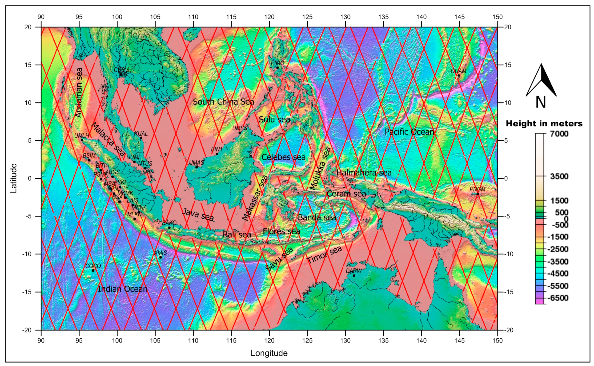
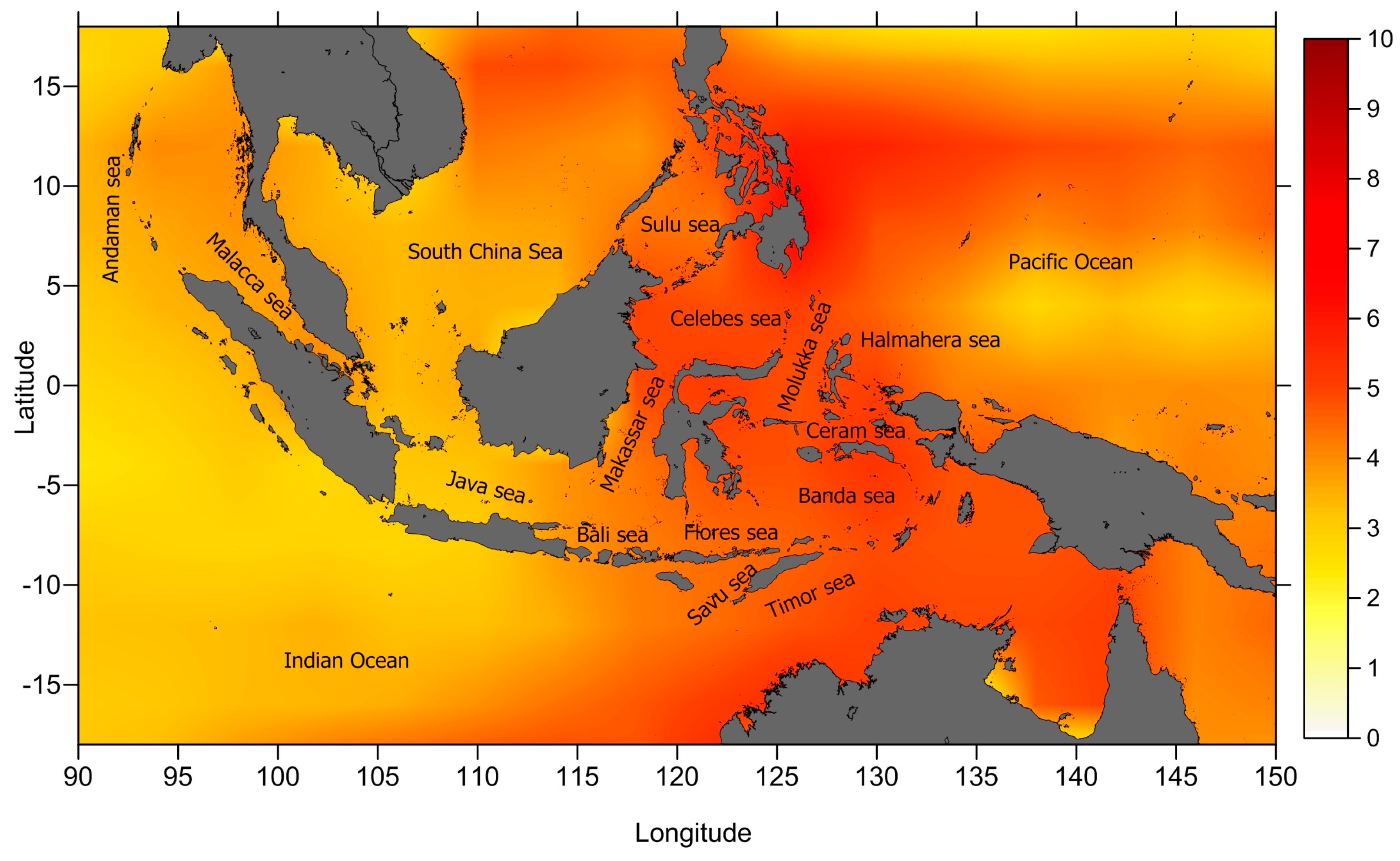
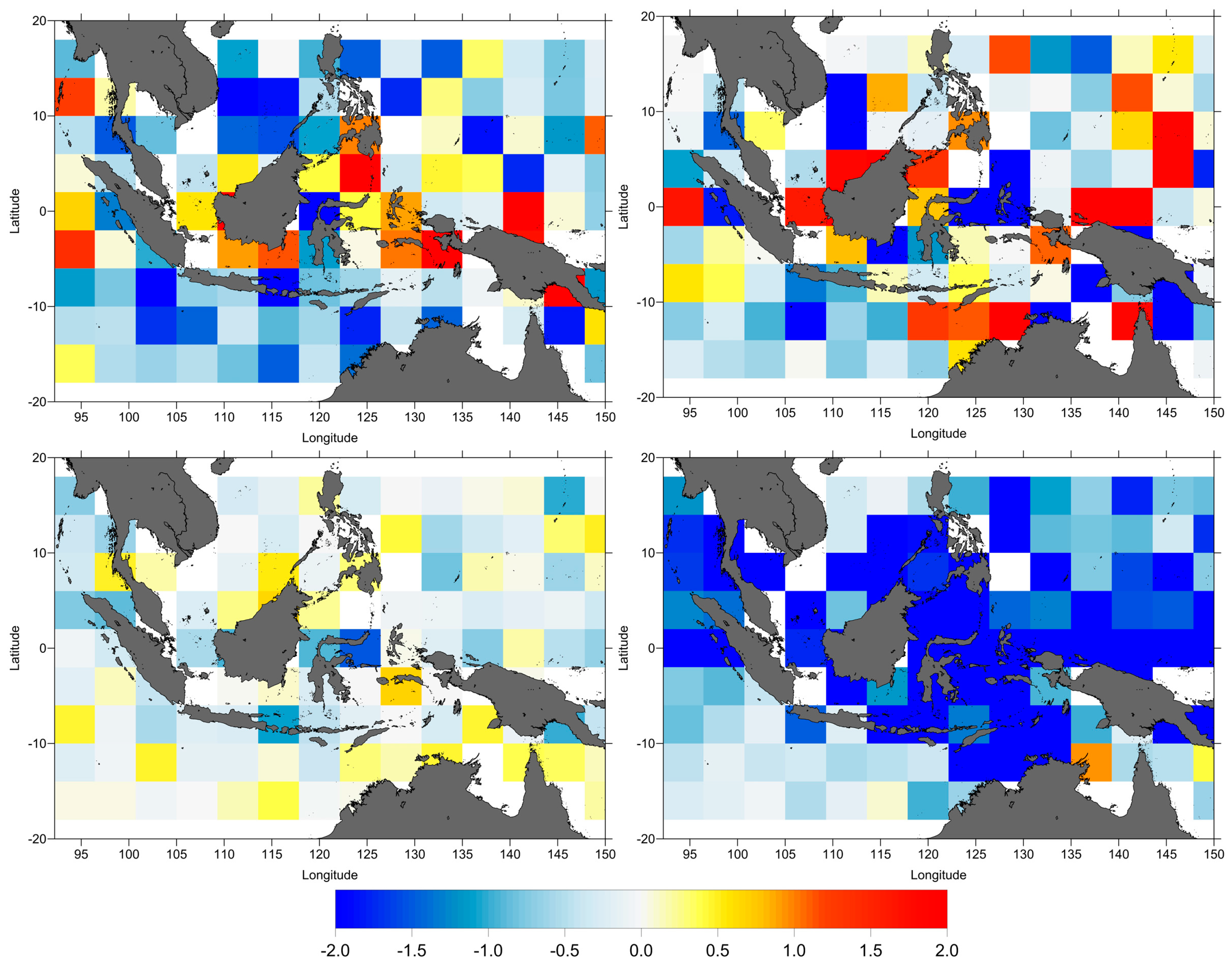
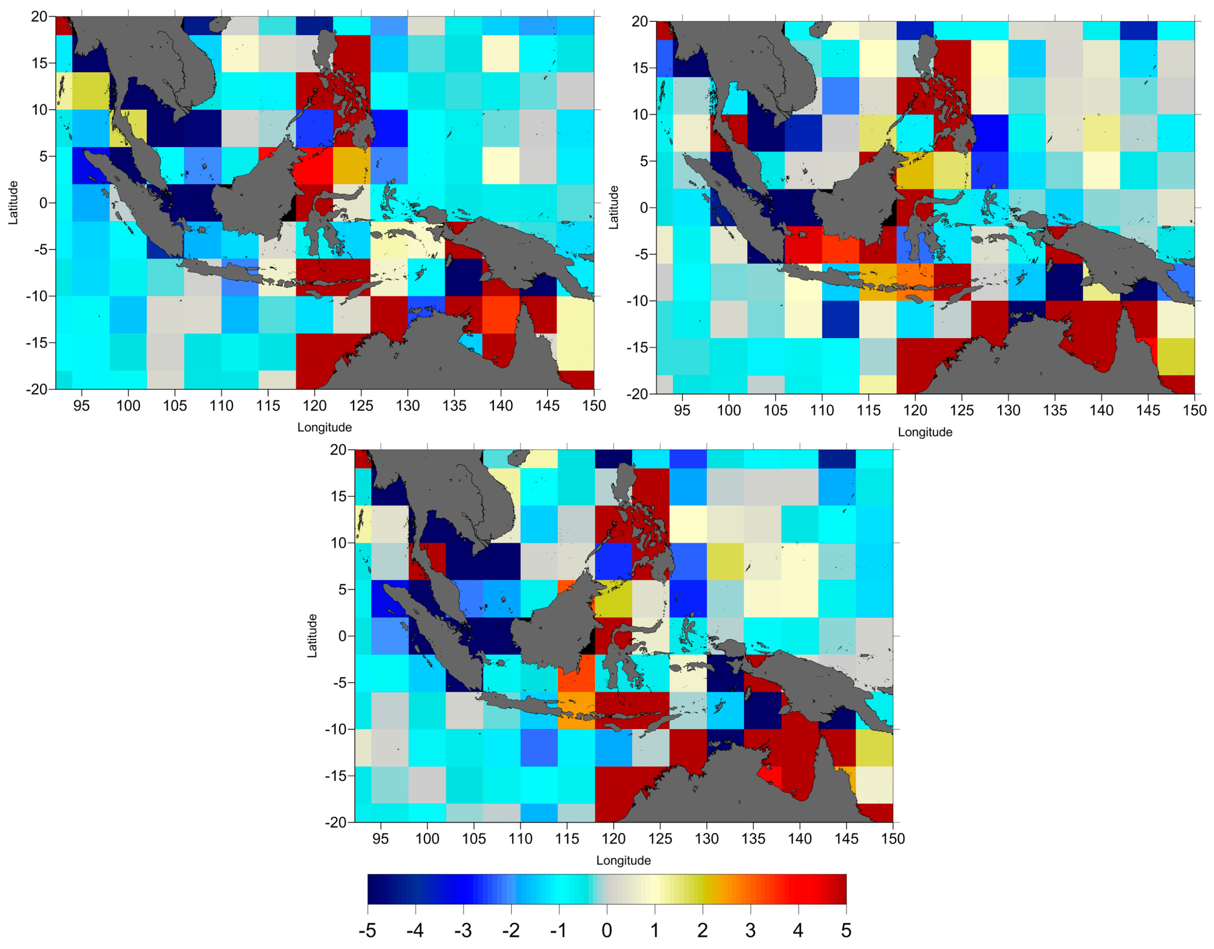
The present study focuses on the analysis of sea level variability in the Indonesian seas for the latitude range 20°S–20°N and longitude range 90°E–150°E. The area covers all the Indonesia seas surrounded by the west Pacific Ocean, the eastern Indian Ocean and the South China Sea (see Figure 1).

In order to investigate the performance of the various range and geophysical corrections and mean sea surface models, several datasets have been prepared. Data from the so-called reference altimetric missions (TOPEX/Poseidon, Jason-1 and Jason-2) have been extracted from the Radar Altimeter Database System (RADS), which is developed by Delft Institute for Earth-Oriented Space Research (DEOS) and NOAA Laboratory for Satellite Altimetry [29]. The data cover a period of more than 23 years (1993–2015).

In this study the analysis of SLA variance, derived from different datasets, was used to study the coastal effects of the various corrections applied to altimeter data and assess their quality. The rationale behind this is the assumption that the more accurate is a range or geophysical correction, the smaller is the corresponding SLA variance estimated using that correction.

The analysis of SLA variance is a common technique to assess the quality of the various terms in Equation (1), which affect the final accuracy of the derived SLA. Using “variance” to measure the dispersion of data is common in statistical analysis. Since variance is a quadratic measure, its values are larger than those for example of the standard deviation, making it easier to detect small differences between the analysed data sets. However, variance is very sensitive to noisy or extreme data values and this can only be overcome by using appropriate criteria for removing those values. This approach has been adopted in this study by applying to the SLA values the standard rejection criteria for example for the acceptable maximum and minimum values for the SLA and for the various range and geophysical corrections used in the SLA computation [28].

The comparison and evaluation of the various range and geophysical corrections and mean sea surface models are performed using SLA variance analysis: along-track analysis (spatial pattern and function of distance from the coast) and crossover analysis. SLA datasets are first derived, for each cycle, using the various corrections or MSS under comparison. Then, in the first case, the difference between the variance of each SLA dataset, computed using all along-track points, is estimated for each cycle. The variance of co-located along-track SLA measurements for a given period and using each correction and MSS, is computed in regular latitude × longitude grids (4° × 4°) intervals (or bins) or in bins of distance from coast and then the differences considered. In the second case, crossovers are first estimated using each SLA dataset, the SLA variance at crossovers is then computed in regular latitude × longitude grids (4° × 4°) and subtracted for selected pairs of SLA datasets. It is commonly accepted in the altimeter community that using SSH crossover differences with a maximum time lag of 10 days reduces the impact of ocean variability, mainly capturing differences due to measurement errors [20,28]; therefore, only crossover points with time difference less than 10 days have been considered. The along-track and crossover variance analyses are two complementary diagnostics, helpful in the assessment of the various analysed variables.

In this study, the following geophysical corrections and mean sea surface models (see

Table 1. Various range and geophysical corrections and mean sea surface models assessed in this study, aiming at determining sea level variability around the Indonesian Seas.

Parameter	TOPEX/Poseidon	Jason-1	Jason-2
Cycles	001–364	001–259	001–280
Dry Troposphere	ERA-Interim & NCEP	ERA-Interim & NCEP	ERA-Interim & NCEP
Wet Troposphere	On-board MWR, ERA-Interim & GPD+	On-board MWR, ERA-Interim & GPD+	On-board MWR, ERA-Interim & GPD+
Ionosphere	Smoothed Dual Frequency & NIC09 (cycles: 1–219), GIM (cycles: 220–364)	Smoothed Dual Frequency & GIM	Smoothed Dual Frequency & GIM
Sea State Bias	Parametric BM4 & Non-parametric: CLS	Non-parametric: CLS & Tran2012	Non-parametric: CLS & Tran2012
Dynamic atmospheric correction (DAC)	MOG2D	MOG2D	MOG2D
Ocean Tide and Loading Tide	FES2012 & GOT4.10	FES2012 & GOT4.10	FES2012 & GOT4.10
Mean Sea Surface	CNESCLS 2011 & DTU2013	CNESCLS 2011 & DTU2013	CNESCLS 2011 & DTU2013

) are evaluated to analyse their impact on sea level estimation:

• Dry troposphere: The dry tropospheric correction (DTC) can be determined from several sources of surface pressure data, such as in situ surface pressure measurements, a Numerical Weather Model (NWM) and a climatology such as the Global Pressure and Temperature Model (GPT) [30]. In this paper, NWM is used to model the DTC due to the limited number and distribution of in situ surface pressure measurements. The most common sources of NWM are the European Centre for Medium-Range Weather Forecasts (ECMWF) and the National Centers for Environmental Prediction (NCEP). For all missions (TOPEX/Poseidon (TP), Jason-1 (J1) and Jason-2 (J2)) the corrections are those derived from the following atmospheric models: (i) ECMWF Re-Analysis (ERA) Interim [31]; (ii) NCEP [32].
• Wet troposphere: the on-board near-nadir-looking microwave radiometer is the best source of information to compute the wet tropospheric correction for altimeter data. The main problem of the MWR-derived WTC in coastal areas is associated with the invalid MWR data measurements due to the large footprint of the instrument that is contaminated by land. Meteorological models are alternative sources to determine the WTC. From these, the ERA-Interim model provides better quality than ECMWF operational model, particularly before 2004 [28,33]. Another WTC source in the coastal zone is the GNSS-derived Path Delay (GPD) corrections provided by the University of Porto. The GPD is an algorithm primarily implemented to estimate an improved WTC in the coastal regions, which combines zenith wet path delay (ZWD) derived from GNSS coastal and island stations, valid onboard microwave radiometer measurements and total column water vapour observations from scanning imaging MWR (SI-MWR) on board remote sensing satellites [27,28,34]. In this paper, the following corrections were used: (i) from the onboard microwave radiometer (MWR); (ii) from the ERA-Interim model; (iii) from the GNSS-derived Path Delay Plus (GPD+) algorithm, the latest GPD version [34].
• Ionosphere: the altimeter satellites TOPEX/Poseidon, Jason-1 and Jason-2 operate in two different frequencies (Ku-band: ~13.6 GHz and C-band: ~5.3 GHz) to determine the ionospheric correction. Three ionospheric models are available in RADS: the JPL (Jet Propulsion Laboratory) GIM (Global Ionosphere Map), NIC09 (NOAA Ionosphere Climatology 2009) and IRI (International Reference Ionosphere). The JPL GIM provides the vertical total electron content (TEC) based on the dual-frequency GNSS data. The GIM is available in two-hourly global grids with a spatial resolution of 2.5° in latitude and 5° in longitude [35]. The NIC09 is a climatology based on the JPL GIM for the period 1998–2008 and variation of solar activity; see details in [36]. The IRI model is a climatology mainly based on ionosonde data measurement since the 1930s. The IRI model has a good accuracy for the northern-mid latitudes, but is less accurate for low and high latitudes, due to poor spatial distribution of ionosode stations [37,38]. According to [36,38], JPL GIM and NIC09 are better than IRI model. Therefore, the ionospheric corrections used in this study for all missions are the smoothed dual frequency and JPL-GIM ionospheric corrections. However, for TOPEX/Poseidon, since GIM is only available since cycle 220, NIC2009 was used for all cycles prior to 220 (1–219).
• Sea State Bias (SSB): In this study, two major types of SSB models usually used in altimetric studies were compared: parametric models, based on three or four parameters and non-parametric models. The SSB correction is commonly estimated as a function of two input parameters: significant wave height and wind speed. In the SBB Tran model [39,40], ocean wave period data are used within a three-input estimator. For TOPEX, the parameter model BM-4 based on [41] and the non-parametric CLS model [42] were applied. The non-parametric CLS and Tran2012 SSB models were applied for Jason-1 and Jason-2.
• Ocean and Load tides: Two main models for ocean and load tides are available in RADS: Finite Element Solution (FES) and Global Ocean Tide (GOT) [43] models. The last version of the GOT ocean and load tide models is GOT 4.10, while one of the latest available FES ocean tide model is FES2012 [44]. The GOT 4.10 load tide should be used to complement FES2012 model since tide loading effects have not yet been computed for FES2012. Therefore, in order to assess the ocean and load tide models, the GOT 4.10 (GOT 4.10 ocean and load tides) and FES2012 (FES2012 ocean tide and GOT4.10 load tide) models were used.
• Mean Sea Surface (MSS): A MSS model is needed to compute the SLA. This study used two MSS models: the CNESCLS2011 [45] and one of the latest releases from DTU (DTU13MSS) [46].
• Other corrections: In addition to the above mentioned corrections, the following were applied: Dynamic Atmospheric Correction (DAC) [47], solid earth and pole tides and reference frame offset [22].

In this study, all corrections were used as they are made available in RADS, except for GPD+, provided by the University of Porto.

In the computations, weighted SLA (weights are function of the co-sine of latitude) were used. Sea level variability around the Indonesian Seas was analysed by combining the time series from TOPEX/Poseidon, Jason-1 and Jason-2. The inter-satellite SLA altimetric series should be calibrated using data for the periods of the tandem phases between consecutive missions. The tandem cycles for TOPEX/Poseidon and Jason-1 are cycles 343–364 and 001–020 respectively, while for Jason-1 and Jason-2 the corresponding tandem cycles are 240–259 and 001–020 respectively. The relative difference between TP and J1 (J1, TP) was determined by averaging the differences between all corresponding tandem mission cycles. Similarly, the relative difference (J2, J1) was determined by the average of the differences from all tandem cycles between Jason-2 and Jason-1.

$$SL{A}_{Corrected}\left(\mathrm{J}1\right)=SLA\left(\mathrm{J}1\right)-bias\left(\mathrm{J}1,\mathrm{TP}\right)$$

(3)

$$SL{A}_{Corrected}\left(\mathrm{J}2\right)=SLA\left(\mathrm{J}2\right)-bias\left(\mathrm{J}2,\mathrm{J}1\right)-bias\left(\mathrm{J}1,\mathrm{TP}\right)$$

(4)

All missions were linked together by applying the computed relative differences in order to determine the 23-year sea level anomaly time series. In addition, the annual and inter-annual signals were obtained using Seasonal Trend decomposition based on LOESS (STL) [48] and the sea level slope was computed by original least squares (OLS).

3. Results

This section presents the results of the impacts of selected corrections and MSS models on SLA estimation, for TOPEX/Poseidon, Jason-1 and Jason-2 altimetry data around the Indonesian seas. The SLA estimated from various corrections (dry troposphere, wet troposphere, ionosphere, sea state bias, tides (ocean tide and load tide)) and mean sea surface models, were compared.

3.1. Dry Tropospheric Correction

The path of the radar altimetry signal through the atmosphere is delayed by the presence of neutral gasses in the troposphere. This effect is called dry tropospheric correction (DTC). The absolute value of the dry path delay at sea level is around 2.3 m. Although the DTC is the largest range correction in satellite altimetry, it can be modelled from surface pressure measurements at sea level (sea level pressure, SLP). Due to the limited number and distribution of in situ measurements, SLP can be acquired from a NWM, such as the ECMWF or NCEP model. Data are distributed on regular grids at six hourly intervals. ECMWF provides two models: the operational model at 0.125° × 0.125° and ERA-Interim at 0.75° × 0.75°, while for NCEP, data are provided in RADS at 2.5° × 2.5°.

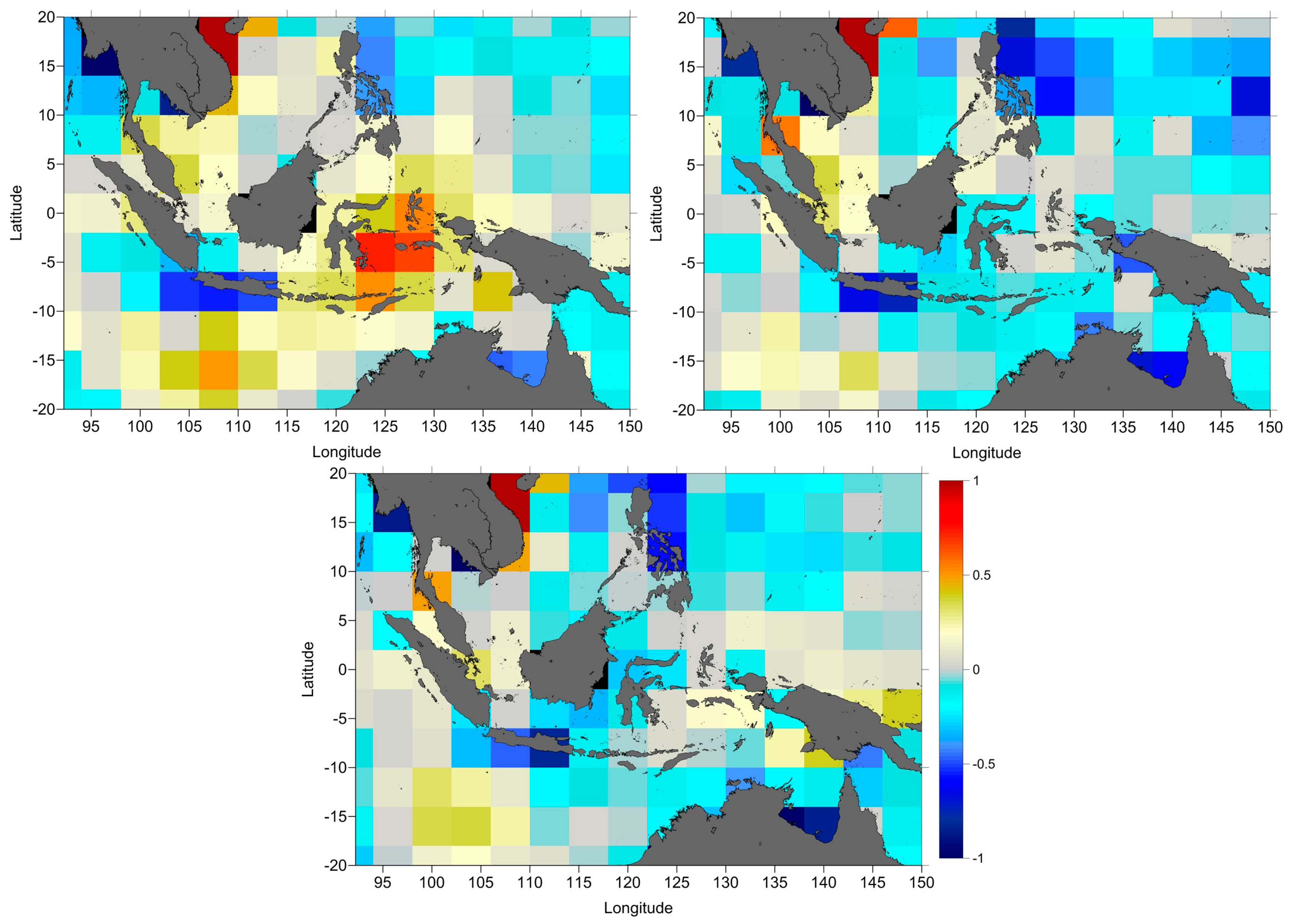
Recent studies indicate that the dry tropospheric correction is not significantly affected by land [22], but it is influenced by the way the height dependence of the corrections is handled [23]. Several authors reported that the accuracy of DTC in coastal areas is about 0.7 cm for T/P [49], Jason-1 [50] and Jason-2 [51]. 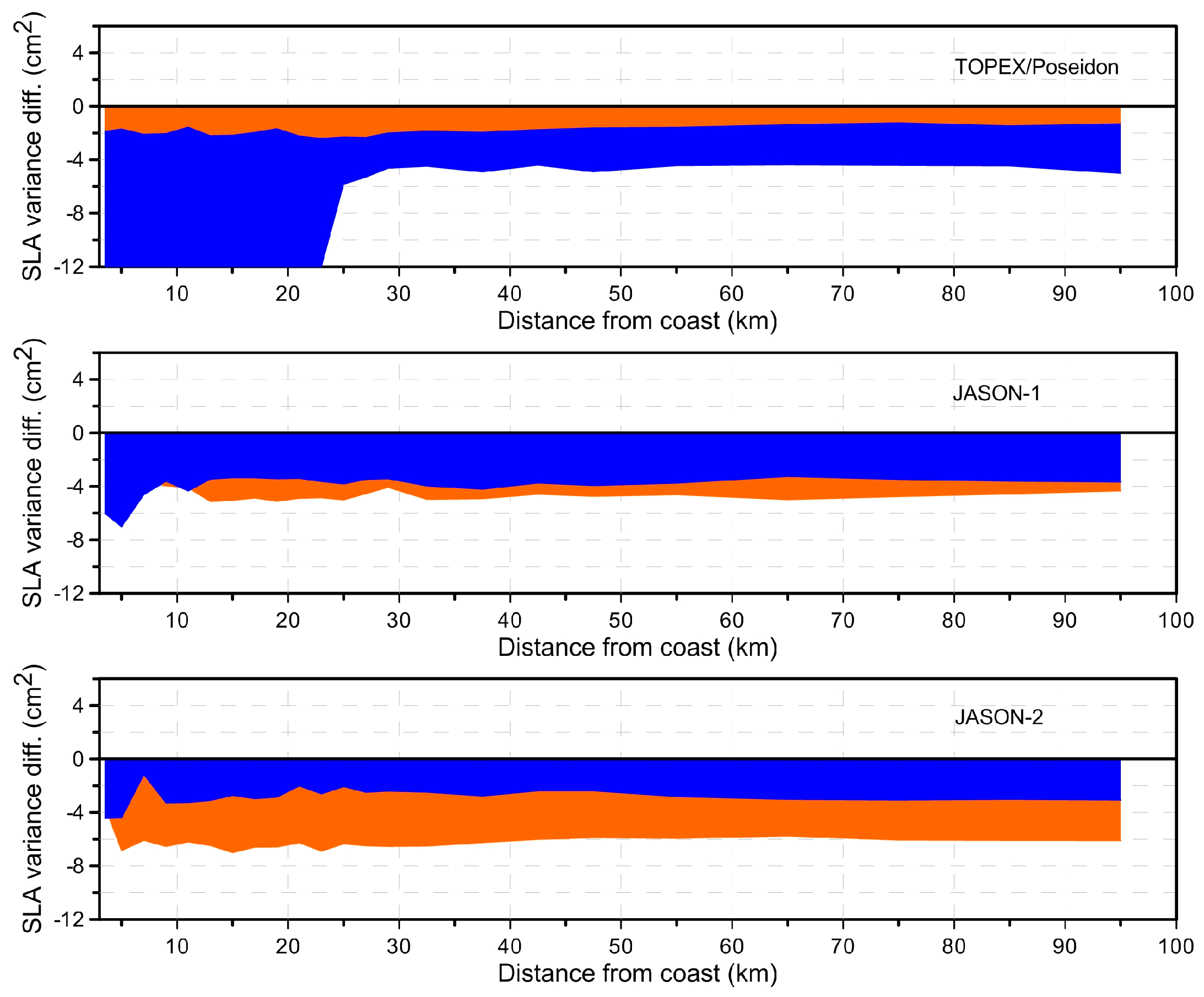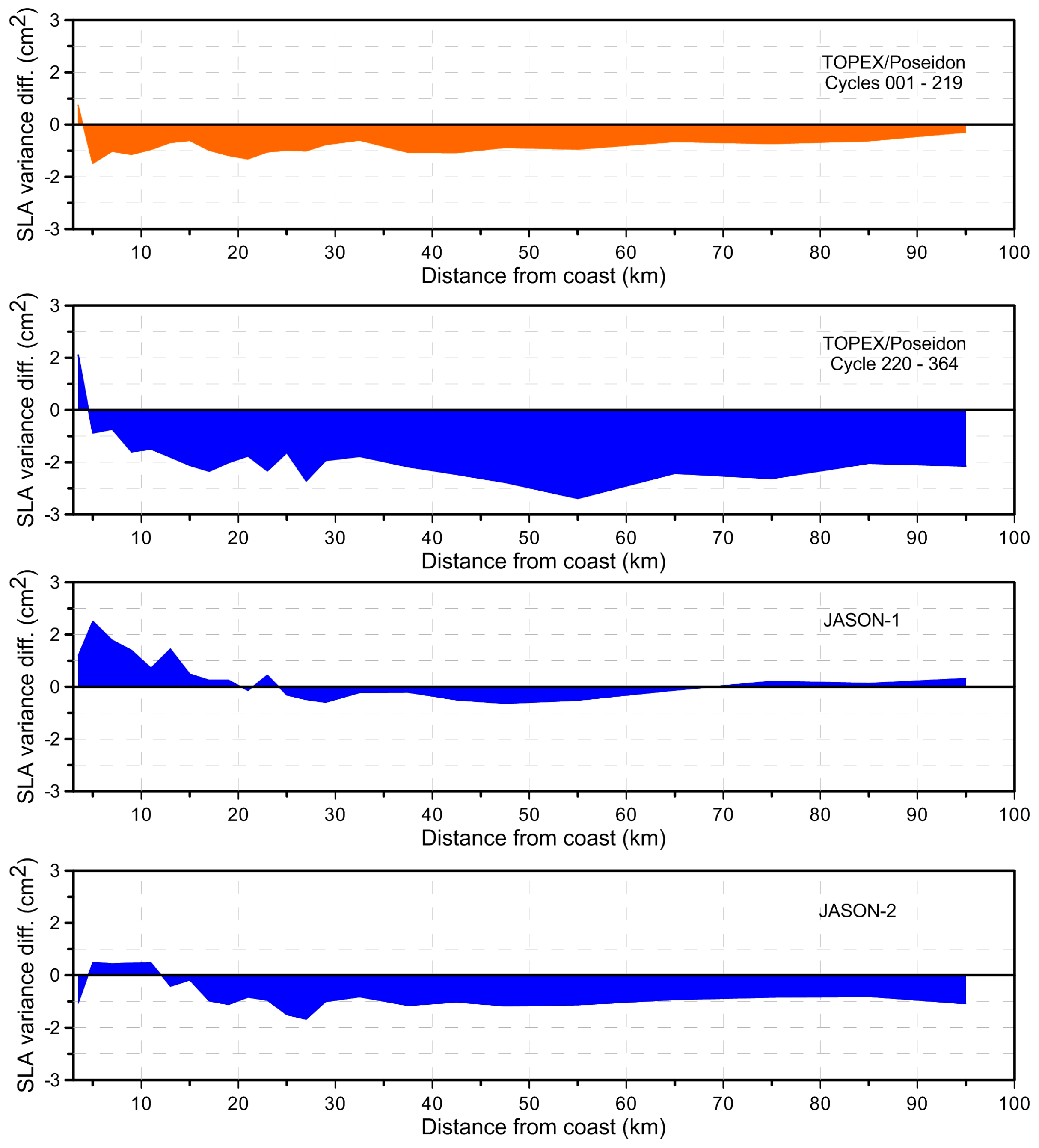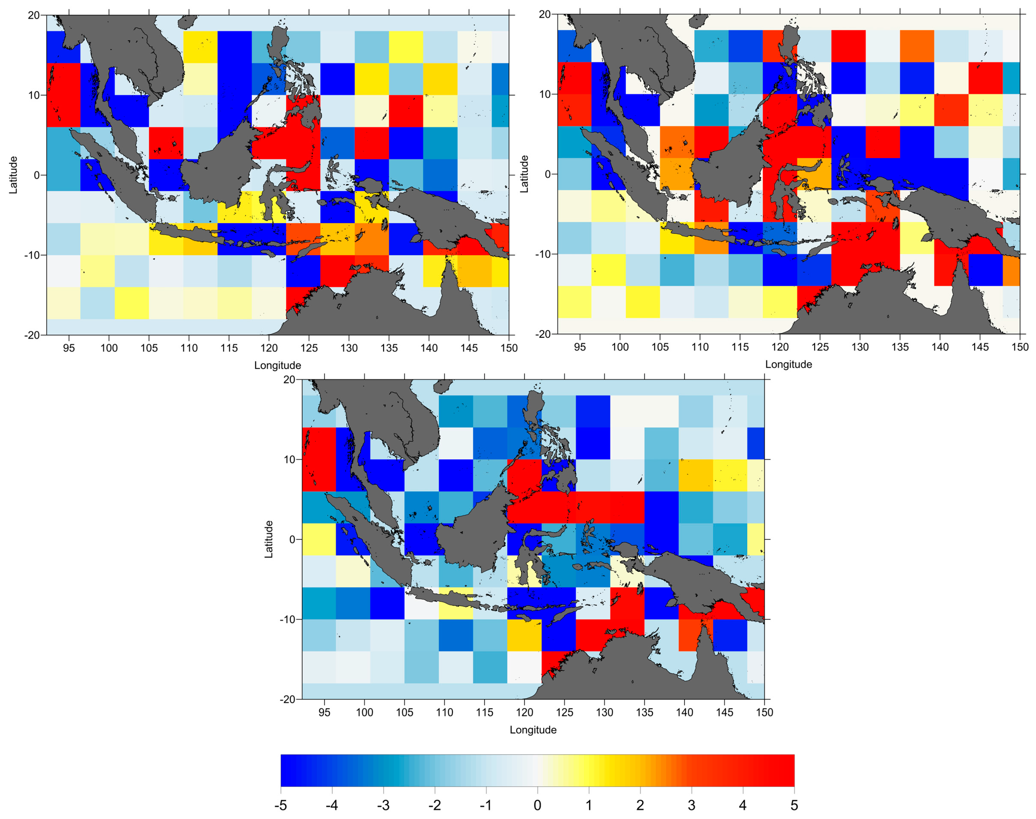Concerning the assessment of the DTC models, SLA variance differences, along-track (Figure 2), function of distance from coast (Figure 3) and at crossovers (Figure 4) between ERA-Interim and NCEP were computed and analysed. Along-track and crossovers SLA variance differences were computed on regular latitude x longitude 4° × 4° grids. In these computations only crossover points with time difference less than 10 days have been considered.

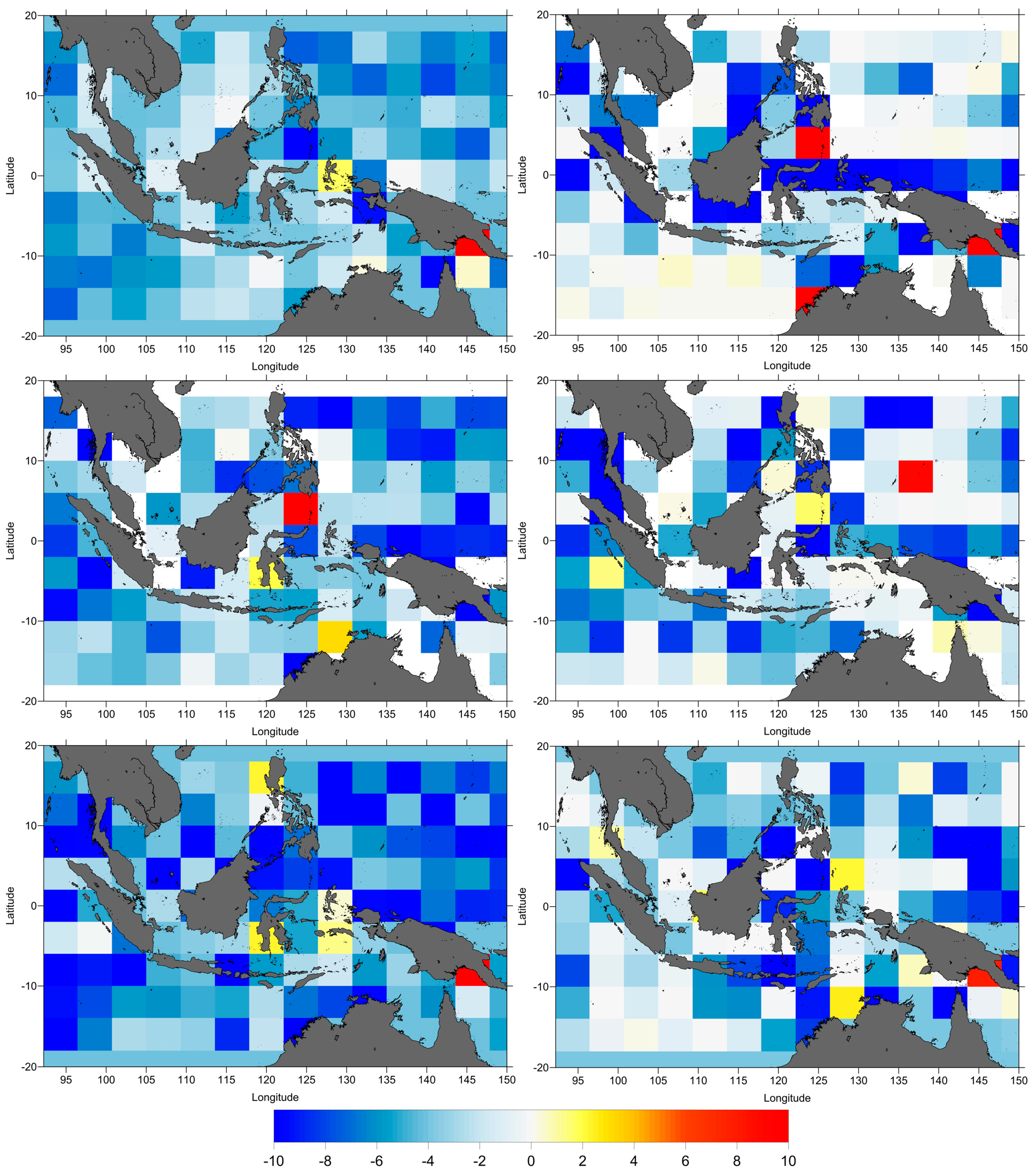
Figure 2 shows the along-track SLA variance differences between two models, ERA-NCEP. It is clear that NCEP DTC is better for TOPEX/Poseidon (shown by yellow to red), but not for Jason-1 and Jason-2 (shown by light to dark blue).

The results in Figure 3 confirm those shown in Figure 2. It shows that NCEP DTC reduces the SLA variance with respect to ERA-Interim model for TOPEX/Poseidon and ERA-Interim DTC reduces the SLA variance with regard to NCEP for Jason-1 and Jason-2. Figure 3 indicates that DTC is unaffected by coastal regions. Figure 4 indicates that the SLA differences at crossovers between ERA-Interim and NCEP are small, mostly negative in open-ocean. This means that DTC from ERA-Interim is better than NCEP in general.

In all cases the variance differences are very small, less than 1 cm². Thus, for consistency, the DTC from ERA Interim should be adopted.

3.2. Wet Tropospheric Correction

For the long-term estimation of sea level, it is important to ensure the consistency and stability of altimetry measurements. One factor that causes uncertainty in satellite altimetry is the path delay due to water vapour in the atmosphere; this is called wet tropospheric correction (WTC). Although the absolute value of the WTC is about 50 cm, it has high variability, both in space and time, and thus is not easy to model.

The wet tropospheric correction is computed from onboard microwave radiometers by measuring the brightness temperature (TBs) at two or three frequencies in the range of 18 and 37 GHz, in spectral bands sensitive to water vapour and cloud liquid water. TOPEX/Poseidon carried the three-channel TOPEX Microwave Radiometer (TMR), which operated at 18, 21 and 37 GHz, while for Jason-1 and Jason-2 the Jason-1 Microwave Radiometer (JMR) and the Advanced Microwave Radiometer (AMR) operate at 18.7, 23.8 and 34 GHz, respectively.

The algorithm for the TMR/JMR/AMR performs the retrieval in three steps. First, a term analogous to a surface “radiometer wind” and a term due to cloud liquid water are estimated using a linear combination of the TBs from the 3 channels. Then, a first approximation of the wet path delay is estimated. Finally, the wet path delay is obtained by adding to the cloud liquid water term a term obtained from a log-linear combination of the TBs from the 3 channels, with coefficients depending on the “radiometer wind” and wet path delay class interval obtained in the first two steps [52].

The radiometer instrument drift can cause an error that will affect the long-term sea level estimation. Concerning the reduction of this potential error, a number of authors have investigated the microwave radiometer instrument drifts [53,54,55,56,57,58,59].

In the open ocean, WTC can be retrieved within a few cm accuracy using onboard microwave radiometers. However, this does not apply to the coastal regions. The differences between ocean emissivity (around 0.5) and land emissivity (around 0.9) cause the radiometer footprint, as it approaches the coast, to contain portions of surfaces with different emissivity. Therefore, the WTC ocean retrieval algorithm originates invalid measurements in the regions close to the coast or land. The invalid data for TMR and JMR start from about 50 km from the coast; while for AMR on Jason-2 begin around 25 km from land [26,60]. However, the JMR and AMR data present on RADS are already enhanced near the coast [26], thus these effects are expected to be much smaller for these satellites when compared to TOPEX/Poseidon.

As an alternative to the WTC from onboard microwave radiometers, a number of atmospheric models, such as ECMWF and NCEP, which provide data on regular grids, can be used to derive tropospheric path delays. Using ECMWF parameters such as sea level pressure (SLP), surface temperature (2-metre temperature, 2T) and total column water vapour (TCWV), the WTC can be calculated. The model grids of WTC are then used to estimate the WTC at each satellite ground track point by bilinear interpolation in space, followed by a linear interpolation in time. The comparison between the WTC derived from the ECMWF operational and ERA-Interim, performed by [28,61] showed that the use of the ECMWF operational model prior to 2004 is not advisable for altimetry studies. For this reason, the ECMWF operational model is not used in this study, only the ERA-Interim, being the best available model for the whole altimeter era.

To reduce the WTC errors, particularly in coastal regions where the onboard microwave radiometer measurements become invalid due to land contamination in the radiometer footprint, a method to determine the troposphere wet path delays, by space-time objective analysis from the combination of data from various sources, was proposed by the University of Porto (UPorto), Portugal (see details in [27,28]. Global GPD solutions have been derived by UPorto for the main altimetry missions (ERS-1, ERS-2, Envisat, TOPEX/Poseidon (TP), Jason-1 (J1), Jason-2 (J2), CryoSat-2 (CS2) and SARAL/AltiKa (SA)) using more than 800 GNSS stations in coastal and island regions [28]. In particular, a local network of nearly 30 GNSS stations, located mostly along Sumatera Island, has been used to improve the GNSS coverage in the Indonesian region (Figure 1).

To ensure the long-term stability of the WTC, the large set of radiometers used in the estimations of the GPD+, the most recent version of these corrections, have been calibrated with respect to the Special Sensor Microwave Imager (SSM/I) and the SSM/I Sounder (SSM/IS). In addition to the inter-calibration with respect to SSM/I and SSM/IS, the new features of the GPD+ corrections with respect to previous versions include: (i) incorporation of additional datasets from a set of 19 SI-MWR; (ii) new grid of spatial correlation scales; (iii) improved criteria for detecting valid/invalid MWR values; (iv) adoption of ECMWF Operational model for computing the first guess of the most recent missions such as CryoSat-2 and Jason-2; (v) adoption of ERA Interim to compute the first guess for older missions such as TOPEX/Poseidon and Jason-1 [34].

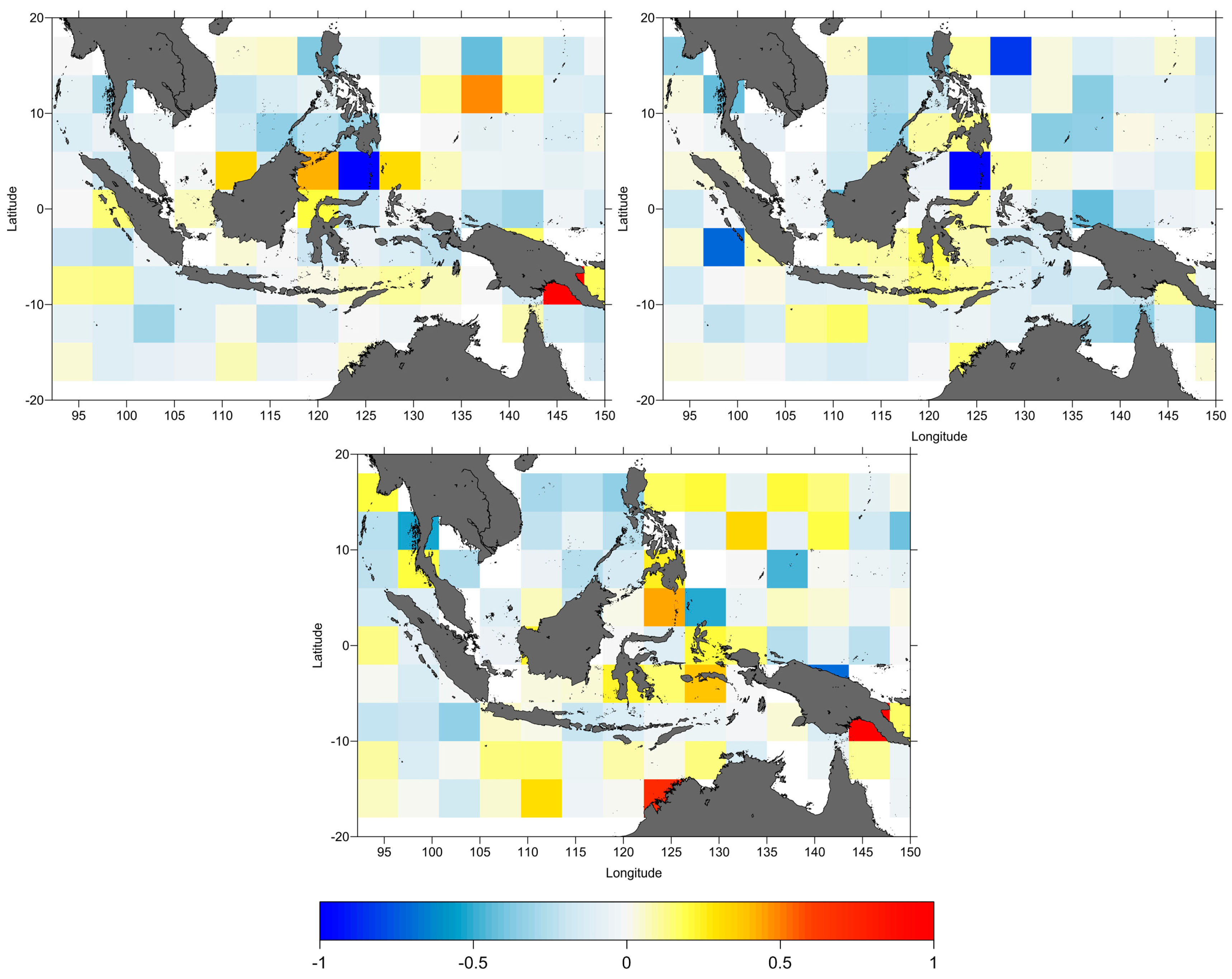
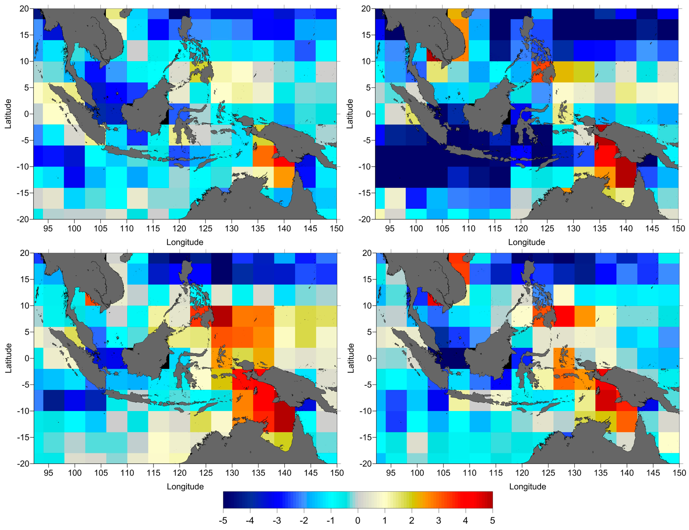
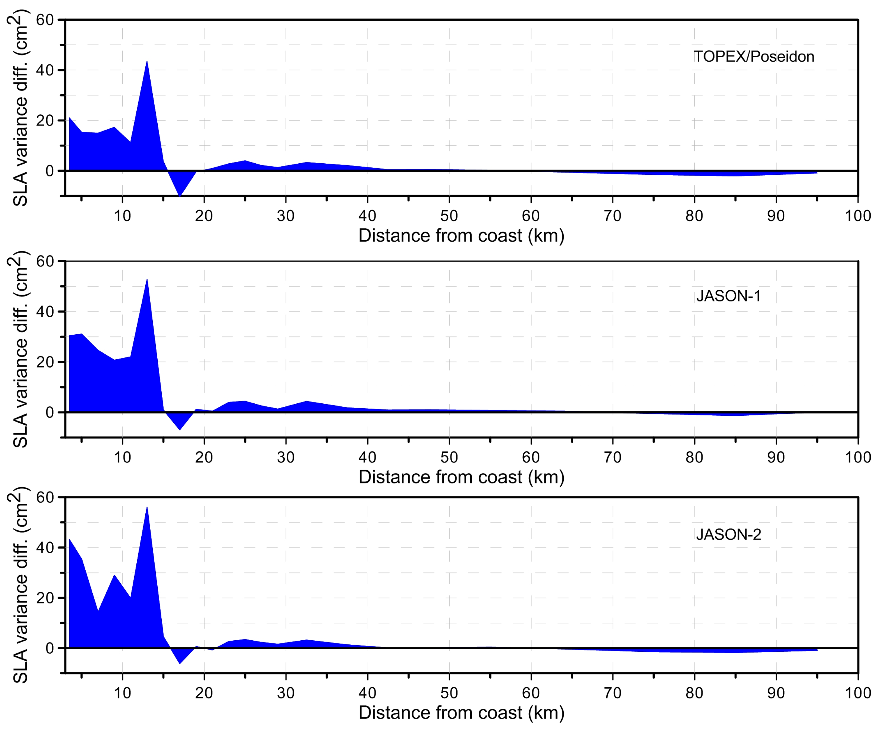
The comparison between the SLA computed using the various WTC, from onboard microwave radiometer (MWR), atmospheric model (ERA-Interim) and GNSS-derived Path Delay Plus (GPD+), was performed. The results are shown as SLA variance differences, spatial pattern of along-track SLA variance differences (Figure 5), function of distance from the coast (Figure 6) and SLA variance differences at crossovers (Figure 7) for all three missions. As before, in these computations only crossover points with time difference less than 10 days have been considered.

Figure 5, Figure 6 and Figure 7 illustrate the results, showing that overall, the GPD+ significantly reduces the SLA variance both with respect to ERA and to the on-board MWR, particularly for TOPEX/Poseidon and near the coast.

3.3. Ionospheric Correction

The ionosphere layer contains free electrons and ions that can influence the propagation of electromagnetic waves both in the speed and in the propagation direction of the signal. The velocity of the signal is slowed by the free electrons in the atmosphere. The ionization process is driven by the sun activity, varies in time of the day, the season of the year and geographical position. The ionosphere delay can be determined in terms of total electron content (TEC), which is the integral of the electron density along the signal path. TEC is measured in Total Electron Content Unit (TECU), with 1 TECU equivalent to 10¹⁶ electrons/m². As a dispersive medium, the ionosphere refraction is frequency-dependent. The ionosphere delay can be determined as function of the frequency [22]:

$$\Delta R_{iono}=k\frac{TEC}{f^2}$$

(5)

where k is a constant of 0.40250 m·GHz²/TECU, TEC is the total electron content, f is the frequency in GHz and $\Delta R_{iono}$ is given in meters.

Satellite altimetry missions such as TOPEX, Jason-1 and Jason-2 carry dual frequency instruments to provide the ionosphere information. The primary frequency, Ku-band, is operating at 13.6 GHz and the secondary frequency, C-band, is at 5.3 GHz. Using two frequencies it is possible to directly detect TEC along the satellite track. Due to the fact that the second frequency is less precise than the Ku-band, the differencing dual frequency creates an additional noise in the derived ionospheric correction which needs to be smoothed around 200 km along the track in order to reduce this error [22].

The global ionosphere maps (GIM) of vertical TEC is an observational model based on more than hundred GPS stations from the International GNSS Service (IGS) network. This model, developed by the Jet Propulsion Laboratory (JPL) and the University of Berne, is available in 2-hourly TEC maps and 2.5° in latitude and 5° in longitude spatial resolution [35]. In addition, NIC09 (NOAA Ionosphere Climatology 2009) is a climatology model based on GIM for the period from 1998 to 2008, which can be applied to estimate the ionospheric correction prior to 1998 [36]. In this study, all ionospheric corrections were used as they are made available in RADS.

In order to assess the accuracy of the ionospheric corrections, two sources were compared; the smoothed dual frequency and JPL-GIM for all missions. Since JPL-GIM has only been available since 1998, for TOPEX prior to 1998 (cycles 1 to 219) the smoothed dual-frequency correction was compared with the NIC09 model.

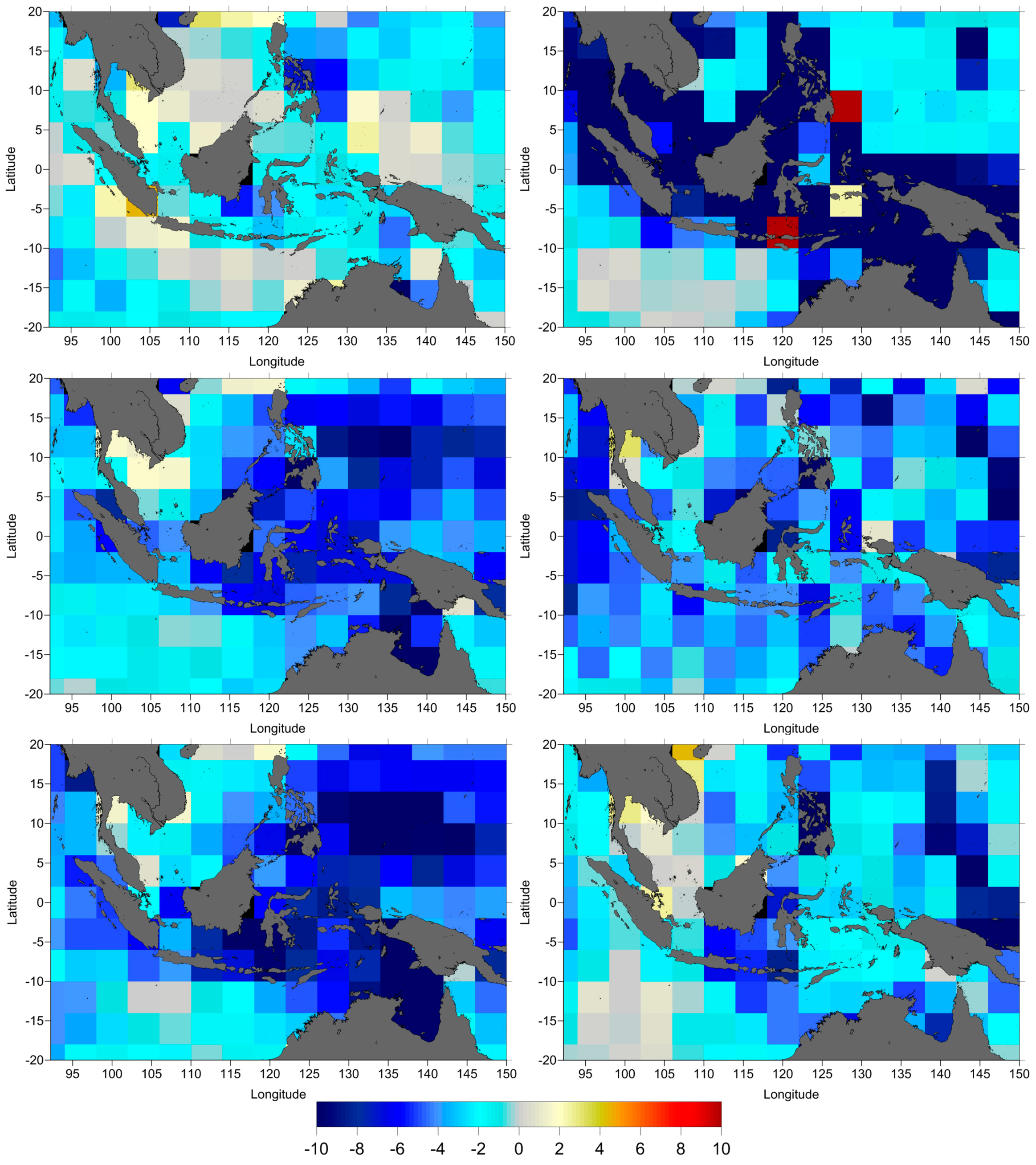
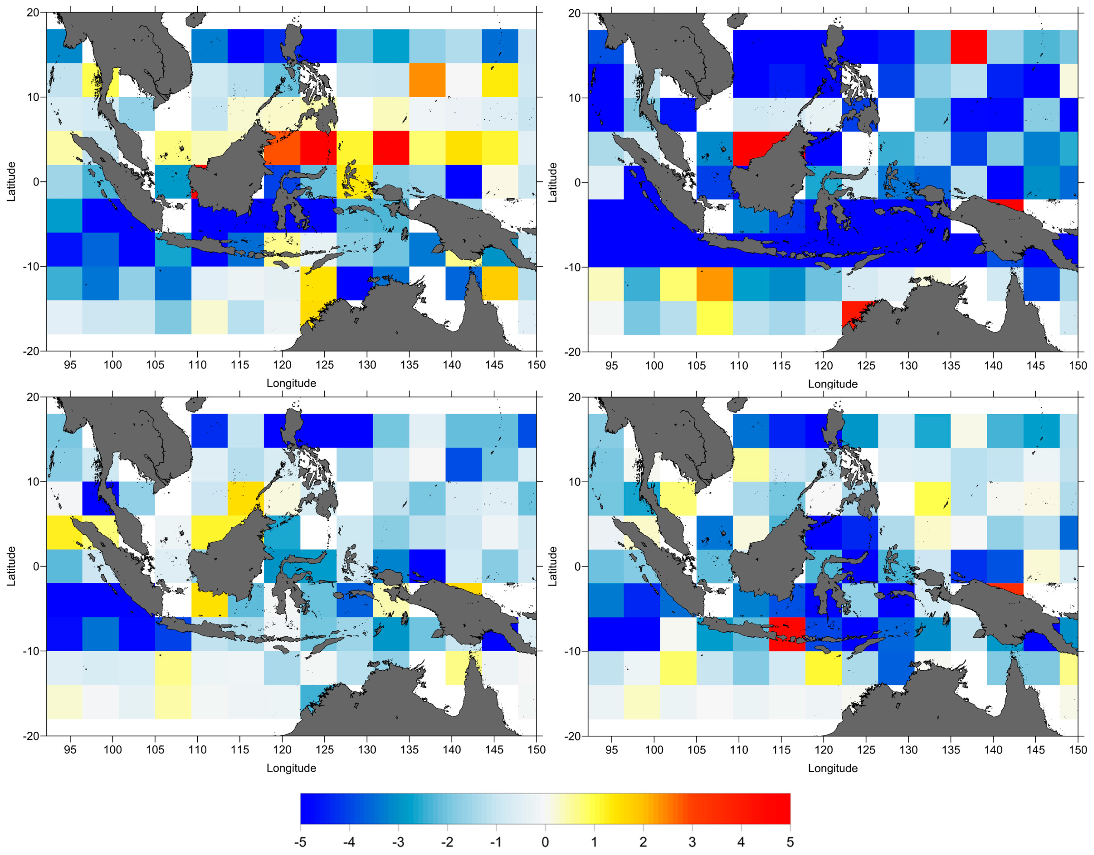
The impact of the ionospheric model in the estimation of the SLA is quantified by plotting the spatial pattern of the along-track SLA variance differences (Figure 8), SLA variance differences function of the distance from coast (Figure 9) and the SLA variance differences at crossovers (Figure 10).

As shown in Figure 8, Figure 9 and Figure 10, in general, the altimeter SLA performances are significantly improved with the smoothed dual frequency (shown as negative variance differences) apart from some degradation sometimes observed near the coast. Overall, the smoothed dual frequency shows a significant improvement when compared with NIC09 and JPL GIM for TOPEX/Poseidon. However, for Jason-1 and Jason-2 the improvements are not uniform, particularly for Jason-1 (Figure 8). For Jason-2, the improvement of smoothed dual frequency begins at 12 km from coast (Figure 9).

Figure 10 displays the spatial distribution of the crossover SLA variance differences. The negative values (blue) indicate that the SLA performances are improved by the smoothed dual frequency correction but that this improvement is not uniform.

3.4. Sea State Bias

Sea state bias (SSB) is an altimeter ranging error caused by the influence of sea-state effects in the radar altimeter measurements, since the surface scattering elements do not contribute equally to the radar return. SSB correction consists of the electromagnetic bias (EMB), tracker bias and skewness. The electromagnetic bias is due to the fact that ocean wave troughs are better radar reflectors than wave crests, thus overestimating the measured satellite-to-surface range. The tracker bias is caused by onboard tracker instrument errors and errors associated with the re-tracking algorithm, while skewness is linked to the effect of a non-Gaussian surface height distribution, inducing an error due to the difference between the determined median sea surface and the true mean sea surface [62,63]. The sea state bias is associated to the ionosphere, due to the frequency-dependent nature of these corrections. An error in the SSB model will cause an error in the ionosphere correction of about 0.175 in scale for TOPEX and Jason-1, function of Ku-band and C-band frequencies [64].

The sea state bias is usually estimated using two-input estimators: the significant wave height (SWH) and wind speed (U₁₀). Parametric models are usually given by three or four parameters, the function of SWH and U₁₀. The coefficients are derived by, e.g., the least square fit of the crossover height differences [41]. The BM4 parametric model is given by the following equation (see also

Table 2. Coefficients of BM4 model for satellite altimetry [41].

Mission	a0	a1	a2	a3	a4
TOPEX A	0.012450	−0.030578	0.002776	−0.002962	0.000127
TOPEX B	0.028889	−0.032113	0.002992	−0.002780	0.000101
Poseidon	0.015731	−0.062778	0.001894	−0.001194	0.000057

):

$$SSB=SWH\left(a_1+a_{2}SWH+a_{3}U+a_4{U}^2\right)$$

(6)

where SWH is the significant wave height (in meters), U is the altimeter-derived wind speed (in meters per second), and a₁, …, a₄ are coefficients of BM4.

The CLS non-parametric sea state bias model was derived by a statistical methodology based on kernel smoothing [62]. Millions of crossover points can be used to estimate sea state bias on a regular grid of wave height and wind speed. This method can resolve the problem of parameter-derived SSB due to the complexity of the relation between sea state bias, wave height and wind speed [65]. The Tran (non-parametric) model, proposed by [39,40], uses three-input estimators, SWH, U₁₀ and the mean gravity wave period (T_m) from a numerical ocean wave model, NOAA’s WAVEWATCH III (NWW3). The Tran model gives a good result by reducing SSH variance at global and regional scales.

In order to evaluate the parametric BM4 SSB and the non-parametric CLS SSB models, the comparison of these models was performed for TOPEX. Due to instrument degradation there were two different TOPEX altimeters, TOPEX_A being replaced by TOPEX_B by the end of cycle 235. TOPEX BM4 SSB was determined using data for TOPEX_A for cycles 1 to 235 (leading to TOPEX_A BM4 coefficients) and data for TOPEX_B for cycle 236 to 364 (leading to TOPEX_B BM4 coefficients). For Jason-1 and Jason-2, the non-parametric Tran2012 and CLS SSB models are compared. The results are shown in Figure 11 (along-track SLA variance differences), Figure 12 (SLA variance differences as function of distance to coast) and Figure 13 (SLA variance differences at crossovers). Results show that, while for TOPEX_A the CLS model is a significant improvement with respect to BM4, for TOPEX_B it has a worse performance. For both Jason-1 and Jason-2, Tran2012 leads to a variance reduction with respect to CLS SSB model. By adding one more estimator, mean gravity wave period (T_m) from a numerical ocean wave model (NWW3), the Tran model (3 Parameters) gives an improvement by reducing sea surface height variance, particularly for Jason-2.

3.5. Tides Correction

The ocean tide dominates the ocean tide signal, representing more than 80% of the total signal. There are several tidal signals which have smaller amplitudes than the ocean tide: load tide, solid earth tide and pole tide. Using appropriate mathematical formulation, solid earth and pole tide can be derived with centimetric accuracy. In the current study, only the ocean tide and load tide are analysed.

Various models for the ocean and load tides are available in RADS. In the absence of a local ocean tide model for the study region the relatively recent models FES2012 and GOT4.10 were used in this research. FES model, developed by Le Provost [65], was determined by using finite element based on bathymetry and tide gauge data. The FES2012 is provided in RADS as a new tide model which replaced the FES2004. FES2012 is an assimilation model which used the altimetry data and tide gauges in addition to the hydrodynamic model. Using more than 1.5 million nodes and high-resolution global bathymetry, this model proved to be more accurate than FES2004 and GOT4.8 particularly in shallow water and coastal regions [44]. The model is distributed on 1/16° grids and consists of 32 tidal constituents. Unfortunately, tide-loading effects have not yet been computed for FES2012; therefore, GOT load tide model should be used to complete the FES2012 ocean and load tide model [44], and GOT 4.10 is used in this study. The other tide model selected for comparison with FES2012 is GOT4.10 which is the newest model from the set of Global Ocean Tide (GOT) models provided in RADS. 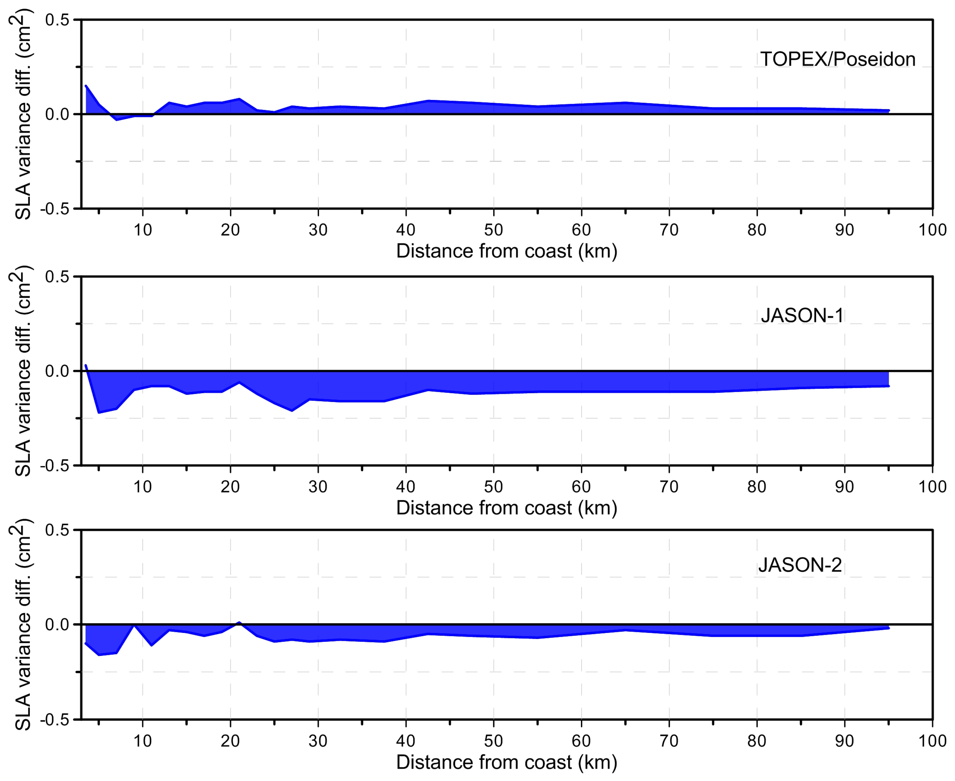GOT models are empirical models derived from satellite altimetry data [43]. In contrast with FES2012 tide model which has 1/16° spatial resolution, GOT 4.10 is provided in rectangular grids 0.5° × 0.5°. The size of grids becomes a problem in coastal regions when the grids do not cover the coastal area. Another version of GOT is GOT-e 4.10c model which has been extrapolated to the shoreline by smoothly extrapolating the GOT4.10 grids. Because no new information has been added, comparisons made for the Indonesia region (not shown) indicate that the GOT-e 4.10c is not more accurate than the original GOT4.10.

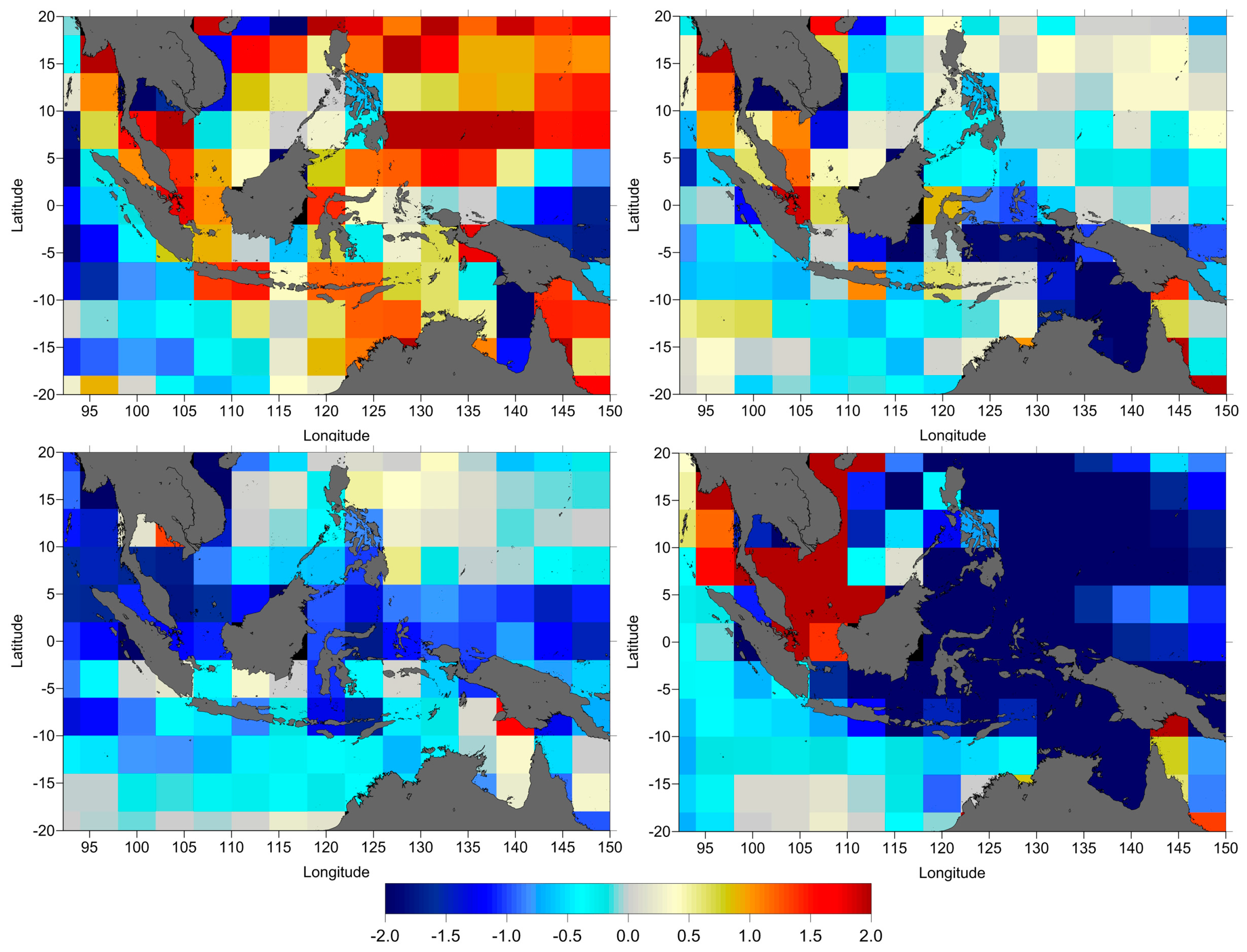
To assess the accuracy of the two models, analysis of SLA variance differences along-track, function of the distance from coast and at crossovers was performed. The comparisons between FES2012 and GOT4.10 are presented in Figure 14, illustrating the along-track SLA variance differences, in Figure 15 showing the SLA variance differences function of distance from coast, and in Figure 16 showing SLA variance differences at crossovers. These indicate that, overall and for all three missions, FES2012 leads to a very large reduction in SLA variance compared with GOT4.10 in the coastal zone, for distances less than 60 km, while in the open-ocean GOT4.10 seems to be better than FES2012.

3.6. Mean Sea Surface

The mean sea surface is the most important reference surface in studies of sea level variation and it is used to estimate SLA aiming at removing the temporal mean of dynamic sea surface topography [66]. The MSS is the sum of the geoid and the ocean mean dynamic topography (MDT), as follows:

$$h_{MSS}=h_{geoid}+h_{MDT}$$

(7)

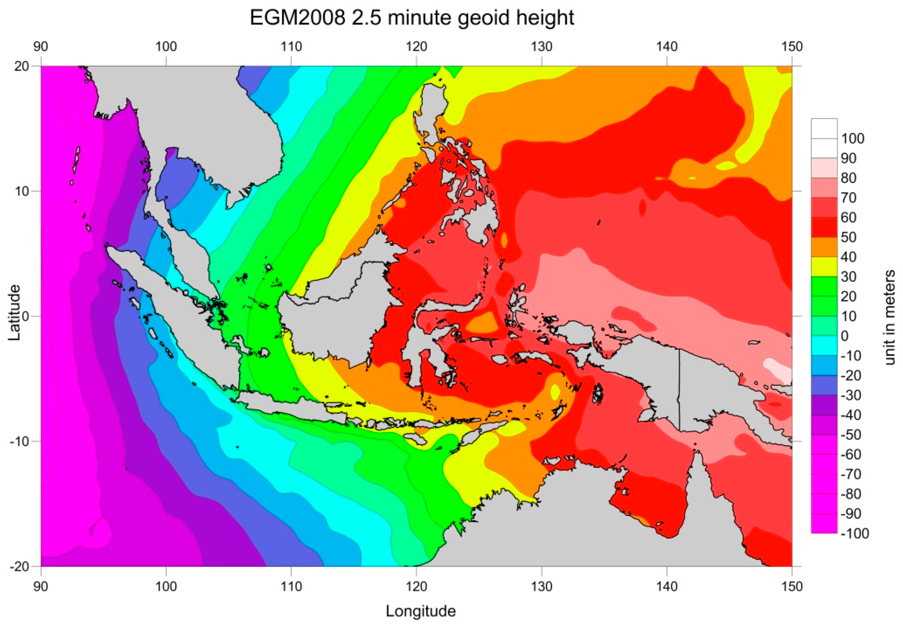
The most recent improvement in the estimation of geoid models consists in using data from dedicated gravimetric satellites, such as the Gravity Recovery and Climate Experiment (GRACE) and the Gravity Field and Steady-State Ocean Circulation (GOCE). The geoid undulation (geoid height above a reference ellipsoid) reaches about ±100 m. In Indonesia, the geoid undulation ranges from −60 m in western Indonesia to +85 m in eastern Indonesia (Figure 17). Unlike the geoid, the MDT has a variation of only a few meters. Therefore, the MSS range variations are very similar to those of the geoid, thus between −60 m and +85 m in the Indonesia region. It is possible to observe that the MSS has large gradients in this region and that the range of the MSS heights above the reference ellipsoid over the study region is close to the maximum range for the whole world. For this reason, the MSS plays a very important role in sea level estimation in this region.

Various MSS models are available in RADS: CNESCLS2011, DTU10, DTU13, DTU15 and EGM2008. In this study, the CNESCLS2011 and DTU13 MSS were chosen. We did not choose the newest DTU15 MSS because, at the time of the writing of this paper, in RADS it was only available for CryoSat-2, Jason-2, Jason-3 and SARAL/AltiKa satellites [29]. The CNESCLS2011 MSS is a mean sea surface model from CLS/CNES, derived from observations covering 16 years of multiple satellite altimeters (TOPEX/Poseidon, ERS-1 Geodetic Mission, ERS-2, Jason-1, TOPEX/Poseidon interleaved mission, GFO and Envisat) [45]. The DTU13 MSS was derived using 9 different satellites for a 20-year period [46]. These MSS models have been compared aiming at assessing model suitability for use in the Indonesian seas.

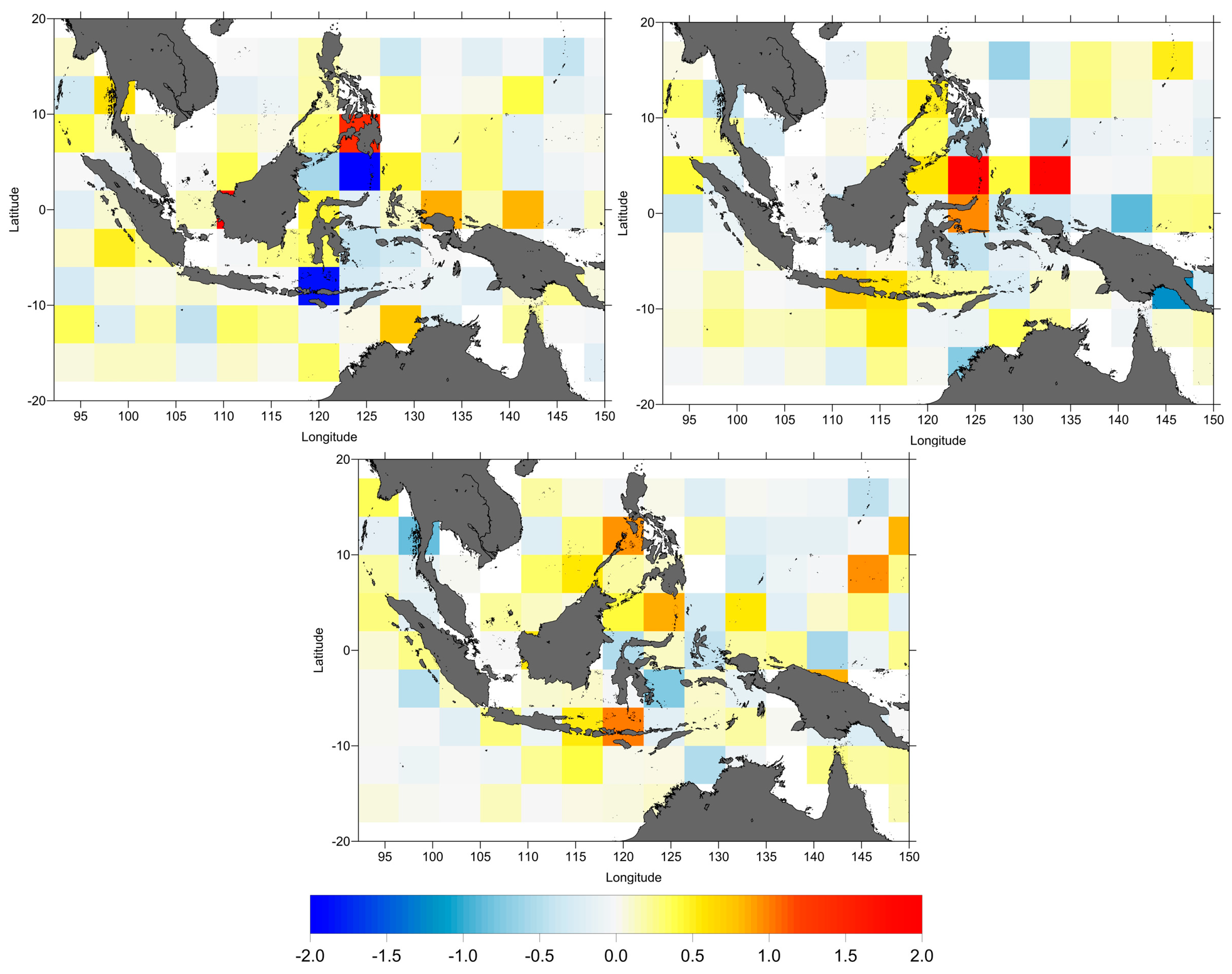
The results for the comparison between the two analysed MSS models (DTU13 and CNESCLS2011) are shown in Figure 18, Figure 19 and Figure 20. In the coastal zone, the CNESCLS2011 MSS reduces the SLA variance significantly for distances up to 40 km from the coast when compared with DTU13 (Figure 19). In the open ocean, the SLA variance differences at crossovers between DTU13 MSS and CNESCLS2011 are small (average less than 2 cm²) (Figure 20) but mainly positive (indicated by yellow to red colours). Due to the nature of the MSS errors, which are time invariant, the along-track SLA variance differences are larger than the corresponding differences at crossovers but also reinforce that CNESCLS2011 is generally better than DTU13 in the coastal regions. The large differences on the coastal areas are mainly due to differences in the methods adopted by each model to extrapolate the MSS values from the sea to land regions.

3.7. Sea Level Variability around the Indonesian Seas

The various range and geophysical corrections and mean sea surface models have been compared and analysed in the previous sections.

Table 3. Selected range and geophysical corrections and mean sea surface model.

	TOPEX/Poseidon	Jason-1	Jason-2
Dry Troposphere	ERA-Interim	ERA-Interim	ERA-Interim
Wet Troposphere	GPD+	GPD+	GPD+
Ionosphere	Smoothed Dual Frequency	Smoothed Dual Frequency	Smoothed Dual Frequency
Sea State Bias	TOPEX_A: BM4	Tran2012 Model	Tran2012 Model
	TOPEX_B: NP-CLS
	Poseidon: BM4
Ocean and Load Tide	FES2012 for <60 km	FES2012 for <60 km	FES2012 for <60 km
	GOT 4.10 for >60 km	GOT 4.10 for >60 km	GOT 4.10 for >60 km
Mean Sea Surface	CNES CLS 2011	CNES CLS 2011	CNES CLS 2011

shows the selected range and geophysical corrections and mean sea surface model for use in SLA estimation in the study region.

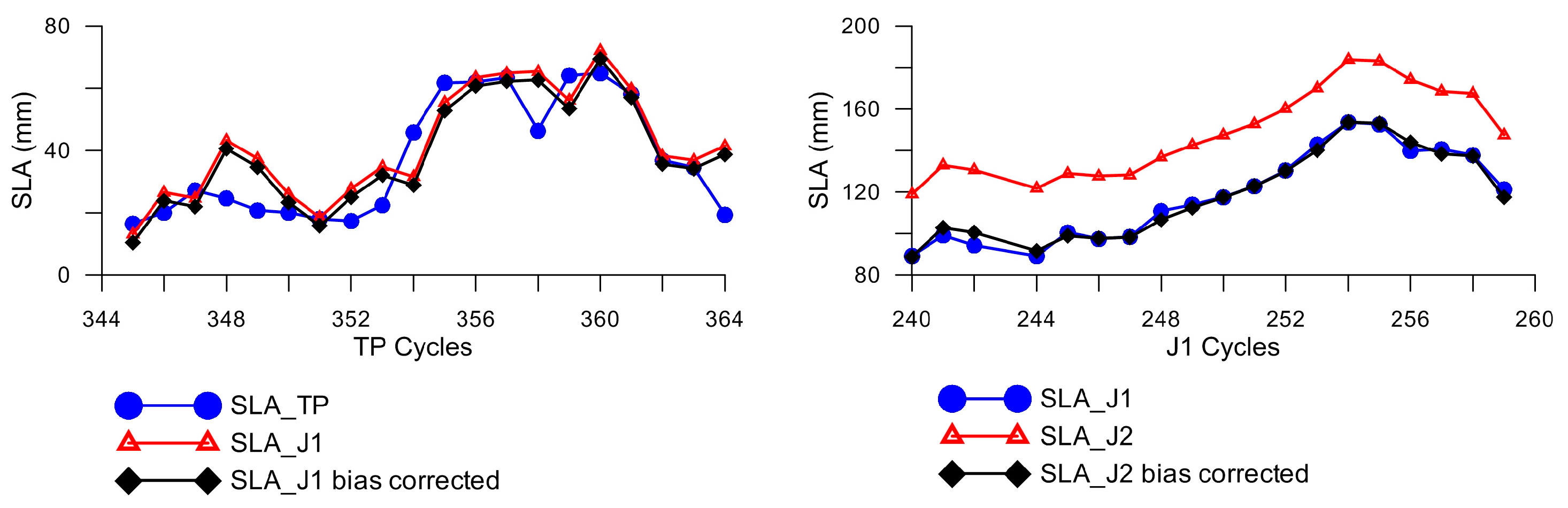
In order to build a continuous SLA time series of TOPEX/Poseidon, Jason-1 and Jason-2 altimetric data, the relative difference between consecutive missions must be applied. The relative differences have been computed by analysing the SLA differences between corresponding cycles of the respective tandem missions as shown in Figure 21. By computing the average difference for the 20 cycles of Jason-1 and TOPEX/Poseidon, a relative difference of 4.6 ± 9.7 mm was found. Similarly, the average of 20 cycle-per-cycle differences of sea level anomaly for Jason-1 and Jason-2 was computed and a relative difference of 30.1 ± 2.7 mm obtained. Despite the fact that the relative difference between Jason-2 and Jason-1 is slightly bigger than the corresponding relative difference between TP and Jason-1, the standard deviation of Jason-2/Jason-1 differences is small and the pattern of the differences between Jason-1 and Jason-2 seems more homogenous. This may be due to the identical instrument of the Jason-1 and Jason-2 altimeters [67], but also mainly due to the fact that different corrections were applied to each mission. Using TOPEX/Poseidon as a reference, relative differences of 4.6 mm and 34.7 mm were applied to Jason-1 and Jason-2 data, respectively.

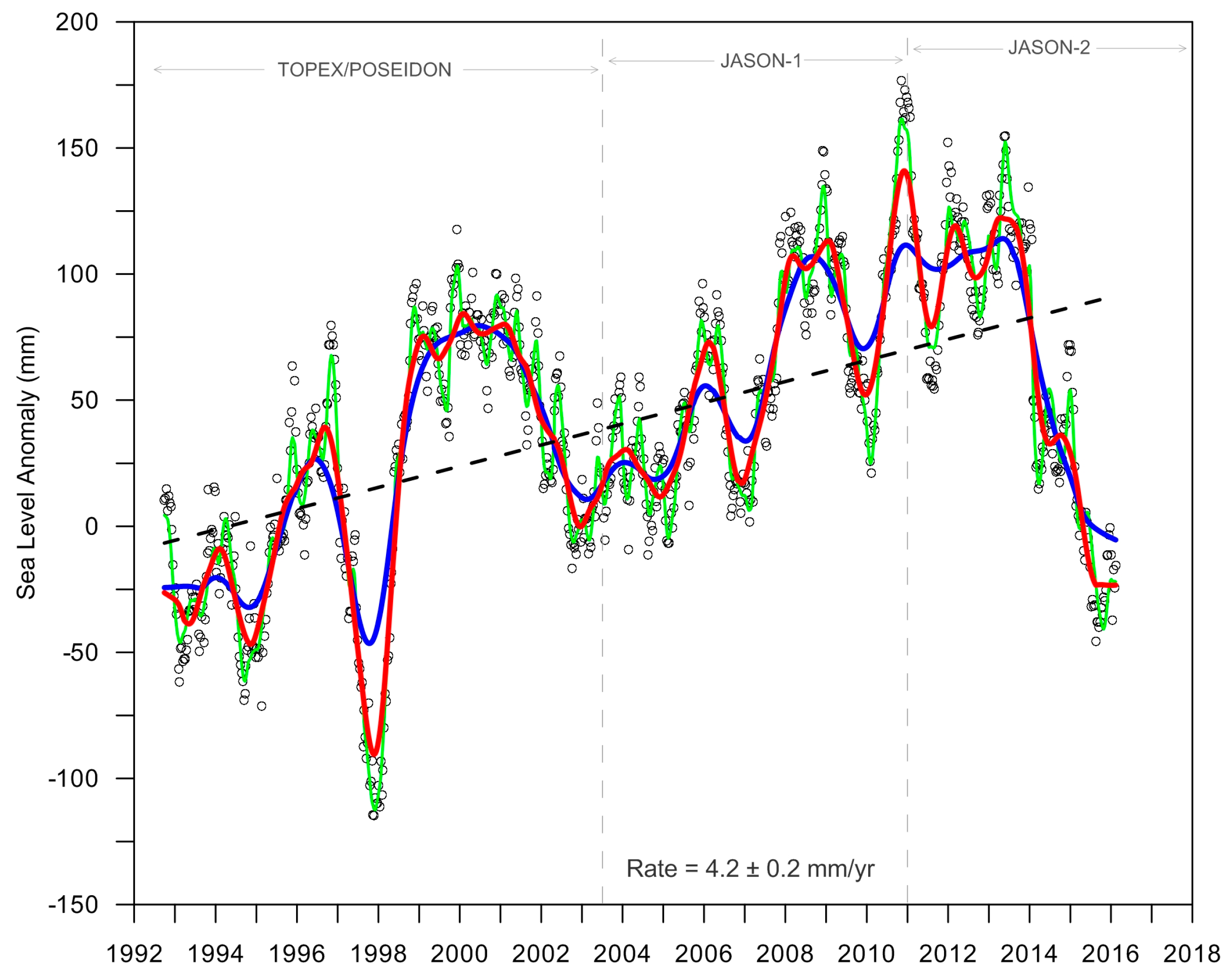
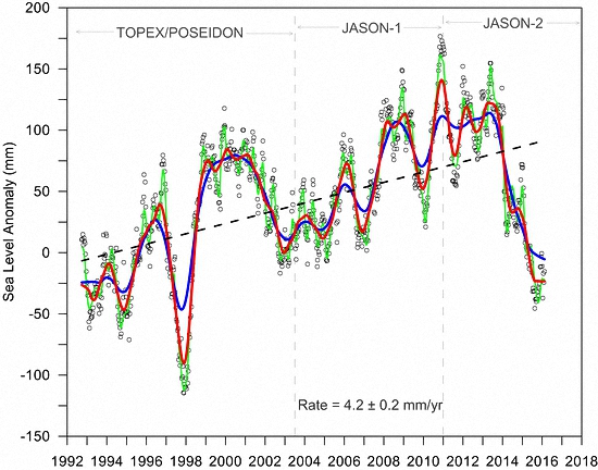
Figure 22 presents the inter-calibrated, relative difference-corrected sea level anomaly time series around the Indonesian seas from all three missions between 1993 and 2015. A 60-day filtering has been applied after removing the seasonal signal (sinusoidal cycle at the annual and semi-annual frequencies) (green line). The raw data are shown in grey dots, the annual variation as a red line and the inter-annual signal is shown as a blue line. The linear trend is computed using least squares. The mean rate of sea level rise is 4.2 ± 0.2 mm/year over 1993–2015.

It has been shown by [68], that some range and geophysical corrections have a direct impact in mean sea level trend estimation. Considering the corrections analysed in this study, the one with the potential largest impacts is the WTC, due to radiometer instrument drifts and instabilities [54]. 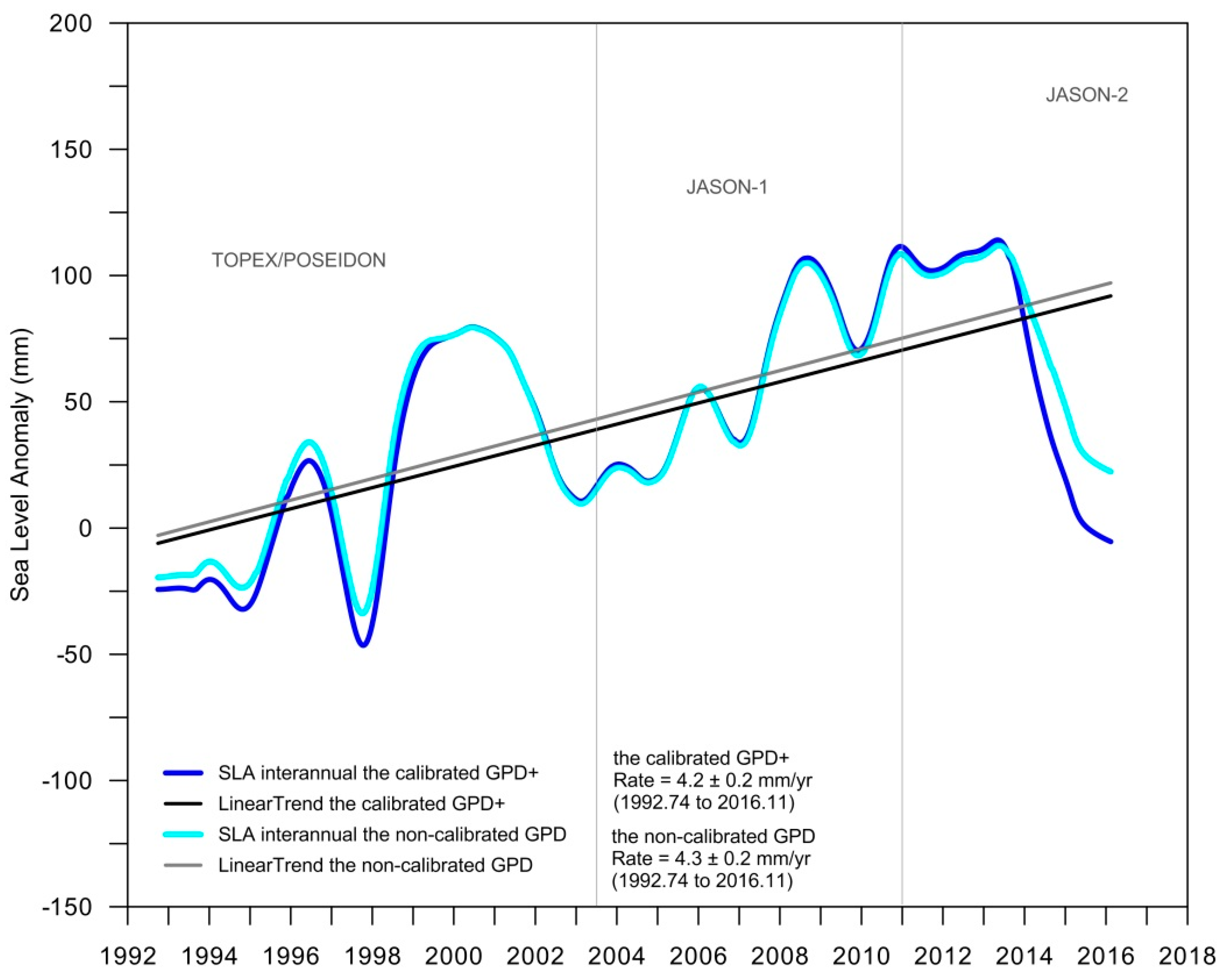Since the GPD+ WTC adopted in this study are a set of corrections that have been calibrated against SSM/I and SSM/IS [34], to investigate the potential impact of this calibration, the mean sea level curve has also been derived with a previous version of these corrections, the so-called GPD, for which no calibration has been performed. The result is shown in Figure 23, illustrating that the difference is very small: 4.3 mm/year for the curve obtained with the non-calibrated GPD versus 4.2 mm/year for the calibrated GPD+ corrections.

Figure 24 shows that the rates of sea level change during the 23-year period (1993–2015) in most areas around the Indonesian seas are higher than the rate of global mean sea level (GMSL). The higher rate is located around the western Pacific (~7 mm/year). The lowest rate is in the Indian Ocean (~2 mm/year).

4. Discussion

Results performed in this study (Figure 2, Figure 3 and Figure 4) show that when considering two different DTC, the SLA variance differences are very small, less than 0.2 cm² near the coast and less than 0.4 cm² in the open ocean, indicating that the DTC impact on SLA estimation is negligible. These results are in agreement with [22] who illustrate that the DTC is unaffected by the presence of land and is not degraded close to the coast. For consistency, DTC from ERA Interim was adopted for all satellites.

Figure 6 shows that for TOPEX/Poseidon, the wet tropospheric correction from GPD+ reveals a significant improvement with respect to the MWR correction present in RADS, particularly near the coast for distances less than 25 km and still has a small improvement with respect to ERA-Interim (less than 2 cm²). For Jason-1 and Jason-2, the GPD+ WTC significantly reduces the SLA variance with respect to the ERA model (about 6 cm²). Regarding the comparison with the onboard MWR-derived WTC, for Jason-1, the GPD+ correction shows a significant improvement (average differences 4 cm²). For Jason-2, the GPD+ correction shows a smaller, still significant improvement (less than 3 cm²), in spite of the fact that this correction is already improved in coastal regions [26].

Figure 5 (along-track SLA variance differences) and Figure 7 (SLA variance differences at crossovers) indicate that GPD+ is an improved correction with respect with ERA-Interim for all three missions, not only near the coast but also in open-ocean. This is expected since GPD+ is based on actual observations, not only from the on-board MWR but also from GNSS and SI-MWR. Results also show that the improvement with respect to ERA is more pronounced for the most recent missions. However, the most significant result is the improvement of the GPD correction with respect to the on-board MWR in the coastal regions, particularly for TP. This is due to the presence of land contaminated and erroneous measurements due to instrument malfunction present in TOPEX/Poseidon data, which rarely occur for Jason-1 and Jason-2 [28]. Figure 23 shows that, for the Indonesian region, while at the time scale of each individual mission GPD+ WTC has noticeable impacts on sea level trend, for the 23-year period the impact is negligible (4.2 mm/year versus 4.3 mm/year).

Regarding the ionospheric correction, Figure 9 shows that, for TOPEX, the smoothed dual frequency leads to a large improvement for all cycles, particularly for cycles 220 to 364 with a variance reduction up to 2.5 cm². Although the ionosphere is insensitive to the coastline, for Jason-1 and Jason-2 the smoothed dual frequency reduces the SLA variance with respect to the JPL-GIM, except for the distances less than 25 km close to the coast. This degradation of the dual-frequency correction in the coastal regions may be due to sea state bias and short-wavelength in the wind field [22]. This may also be due to remaining land contamination still present in the smoothed dual frequency correction. The figures with the along-track SLA variance differences (Figure 8) and at crossovers (Figure 10) show that for TOPEX (cycles 1 to 219), Jason-1 and Jason-2, the smoothed dual frequency does not improve the results homogeneously for the whole Indonesian region, particularly in the Banda Sea, Ceram Sea and Western Pacific and in the Indian Ocean which coincide with unstable regions of the ionosphere [22].

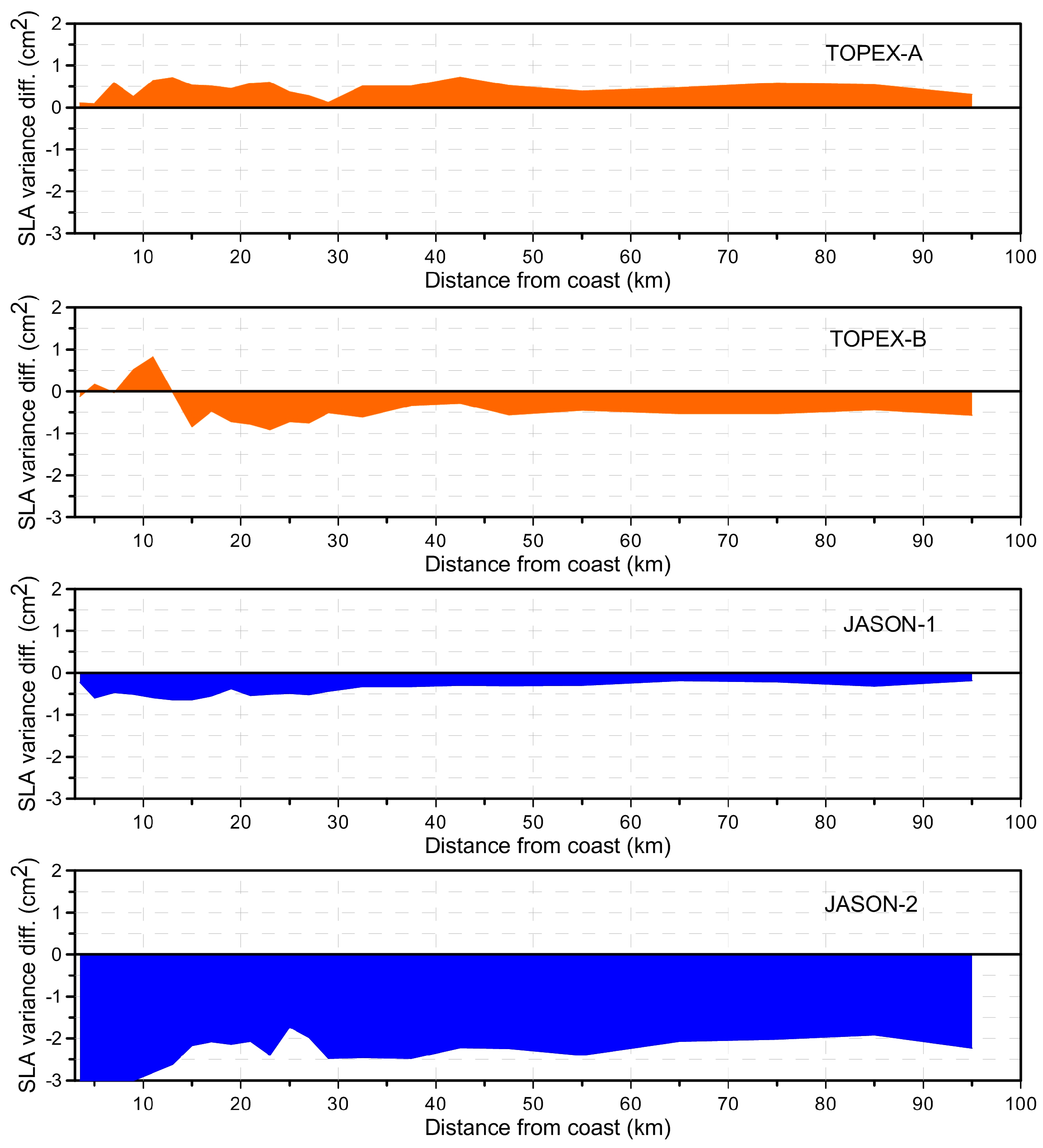
Regarding the SSB correction, Figure 12 shows that, for TOPEX_A, the BM4 parametric model reduces the SLA variance when compared to non-parametric CLS SSB by an average value about 0.5 cm²; in contrast, TOPEX_B non-parametric CLS sea state bias significantly reduces the SLA variance with respect to BM4 parametric model by about 1 cm² with a larger reduction near the coast. For Jason-1 and Jason-2, Tran2012 model shows a significant reduction of the SLA variance when compared to non-parametric CLS SSB, indicated by negative values. The average of SLA variance differences between Tran2012 and CLS SSB (Tran2012 minus CLS SSB) in coastal areas, for Jason-1 is less than 1 cm² and for Jason-2 is about 2.5 cm². Figure 11 and Figure 13 also indicate that the differences between the non-parametric CLS and parametric BM4 SSB have a coastal signature. For TOPEX/Poseidon, SSB CLS slightly increases the SLA variance near the coast (indicated by colours in the yellow to red range). For Jason-1, the SLA variance differences at crossover show that Tran2012 model is a small improvement with respect to CLS SSB. A significant reduction in SLA variance at crossovers is shown for Jason-2 when SSB Tran2012 model replaces the SSB CLS model (indicated by light to dark blue colours). In addition, for Poseidon (PN), BM4 SSB reduces the SLA variance with respect to BM3 SSB by about 3 cm² (the result is not shown).

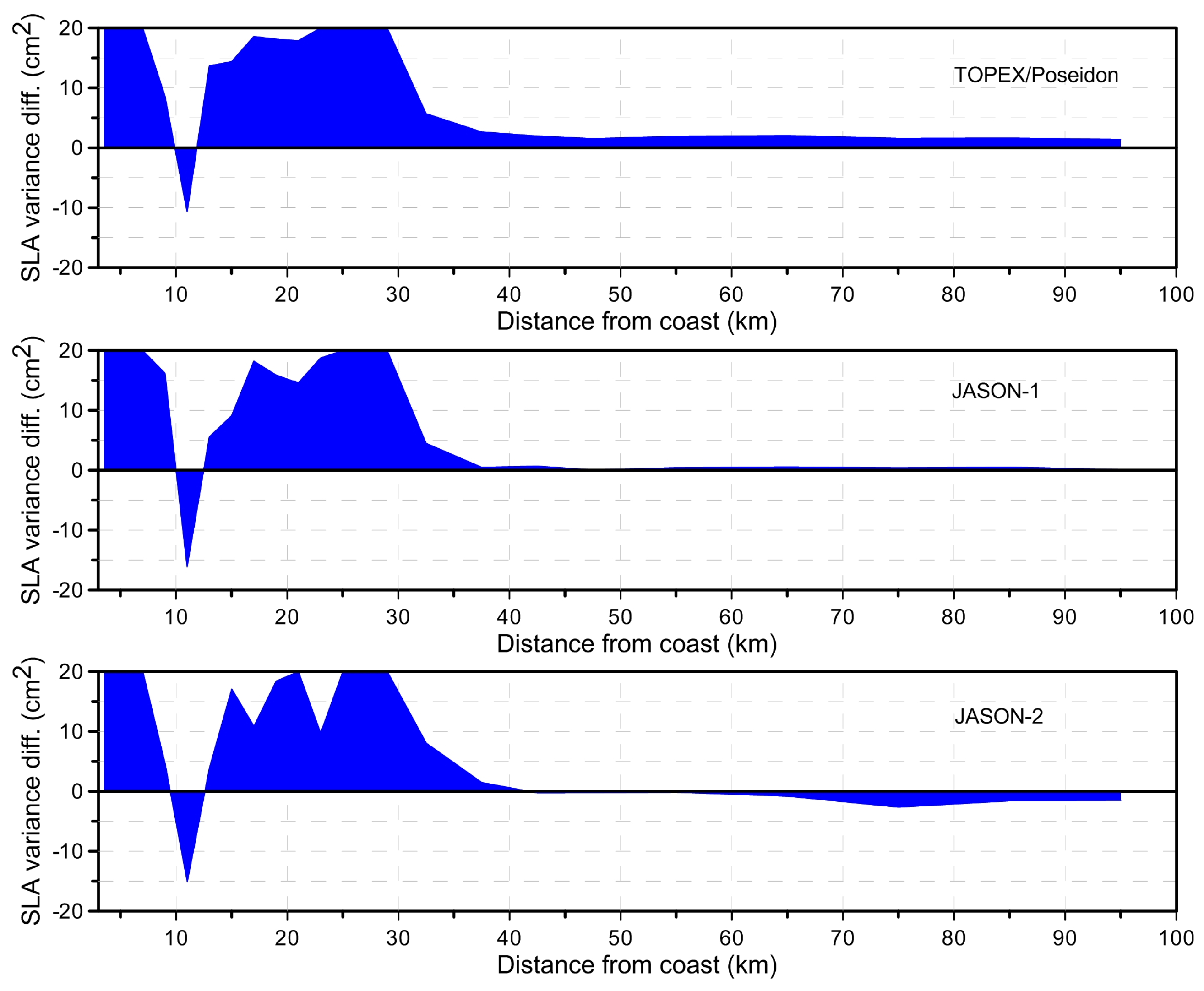
Figure 15 shows that FES2012 tide model significantly reduces SLA variance compared with GOT4.10 in the coastal zone, for distances up to about 60 km from coast, for all three missions. These results are similar to those by [44], for the comparison of SLA variance between FES2012 and GOT 4.8, who reported significant differences between the models near the coast (less than 60 km from coast). However, FES2012 shows lower performances in some areas due to the lack of assimilated data (no data were available for assimilation in the southern Ocean). Although FES2012 model shows good improvement in the coastal regions, the same does not happen in the open ocean, as shown in Figure 14 and Figure 16. When compared with FES2012, GOT4.10 tide model generally reduces the SLA variance at crossovers in the open ocean and increases it near the coast. The largest differences between the two models occur around deep seas, such as Celebes Sea, Ceram Sea, and Banda Sea. This is partly due to the fact that the grids of the GOT models, which are provided at 0.5° × 0.5°, do not extend to the shoreline everywhere, making it problematic to utilize GOT for tidal corrections in the coastal zones, while in FES2012 model more than 1.5 million nodes were used up to the coast. According to the results from the comparison of tide models in this research (Figure 18, Figure 19 and Figure 20), the global tide models can have very large differences in the coastal zones, suggesting that local tide models are required to account for local ocean variability. Unfortunately, no local tide model is available for the Indonesian region.

Concerning the MSS, results for the study region show that CNESCLS11 leads to a large reduction in along-track SLA variance with respect to DTU13, particularly near the coast for distances up to 60 km. As expected, the results are the same for all satellites, since a given MSS model is a time invariant field.

According to [45], the comparison between CNESCLS2011 MSS with a previous DTU model (DTU10) showed that the DTU10 MSS is less well adjusted for ocean variability studies. The high differences between CNESCLS2011 MSS and DTU10 MSS occur mainly near the coast and at high latitudes. A change in the mean sea surface model adopted in the computation of the SLA affects the SLA variance in a different way than a change in a range or geophysical correction. While e.g., two different WTC affect both the temporal and spatial variability of the sea level, a change in the MSS only affects the spatial variability, the temporal variance at each point remaining constant. In spite of that, Figure 18, Figure 19 and Figure 20 show that the change in the mean sea surface has a strong impact in this region, particularly in the coastal regions. 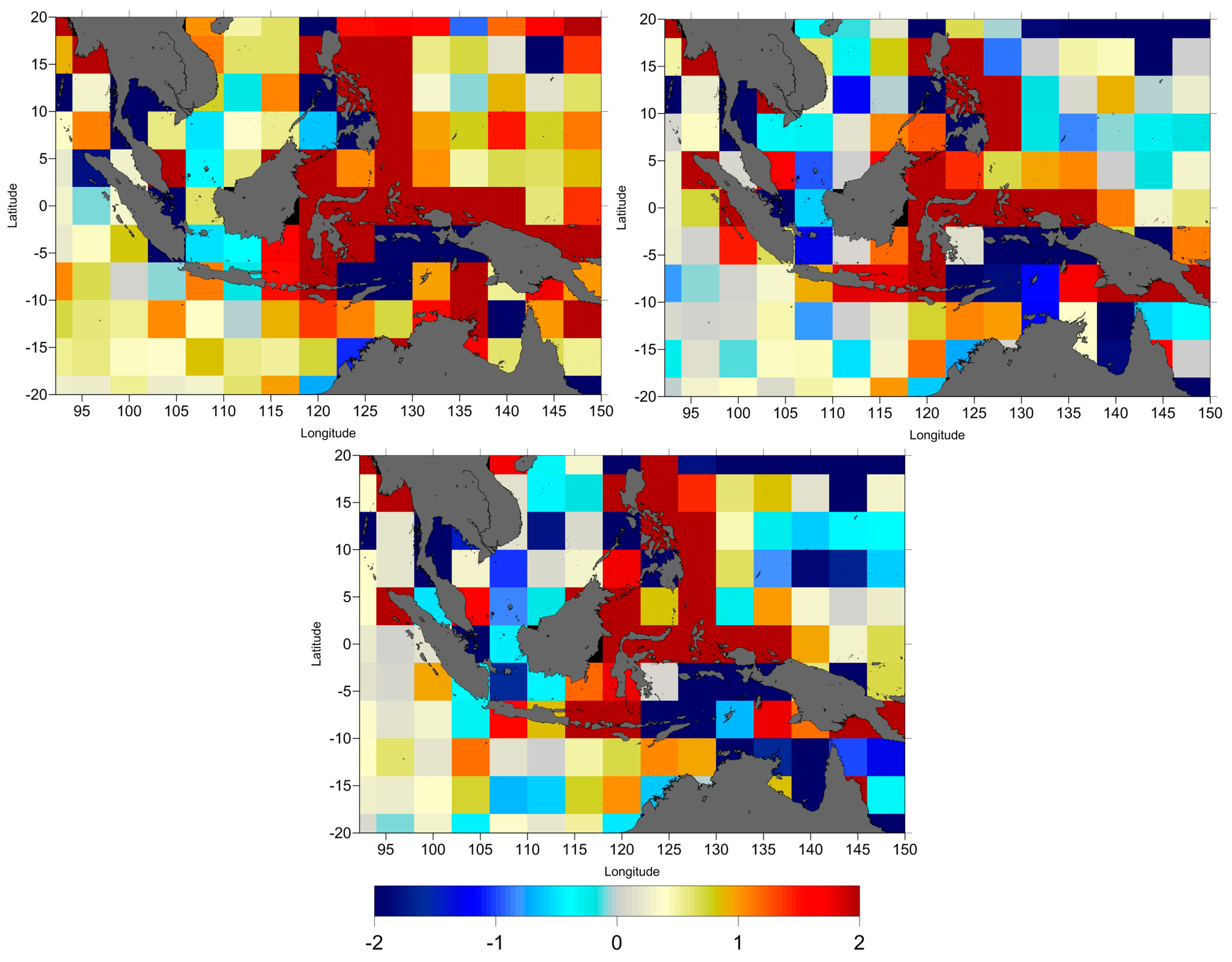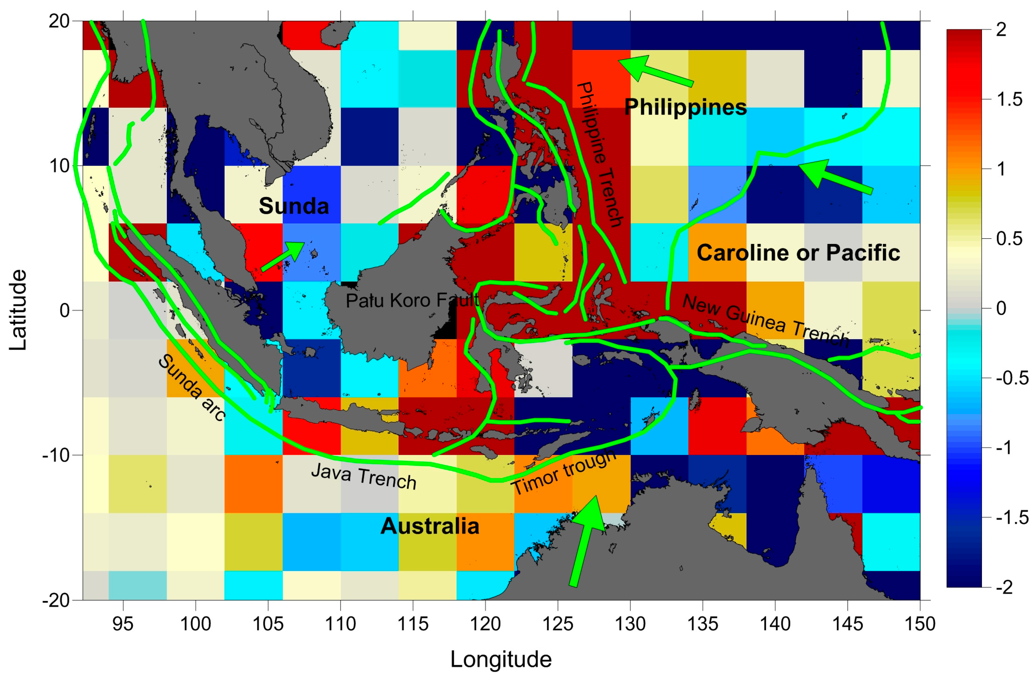Figure 20 illustrates that the largest differences between DTU13 and CNESCLS2011 MSS occur on the triple junction area, the junction of the Sunda-Australia-Philippine-Pacific plates. The triple junction area between the island of Sulawesi and the Moluccas in the eastern Indonesia is highly seismically active and presents a very complex tectonic scenario (shown as Figure 25) [69]. The activities of plates will affect the gravity and geoid changes. Since the MSS is correlated with the geoid (Equation (5)), changes in the geoid will have impact in the determination of the MSS.

The global impact of the El Niño-Southern Oscillation (ENSO) event affects the inter-annual variation of GMSL, particularly over the tropical and sub-tropical Pacific Ocean [16]. ENSO phenomenon is an important component of global climate change, characterised by the appearance of warmer surface water along the equatorial Eastern Pacific Ocean at 2–7 years intervals that can change the precipitation rate, temperature and water vapour during that period. Its effect on the Indonesian seas is significant. The Indonesia seas are considered an oceanic pathway for the Pacific and Indian Oceans where the waters from the Pacific Ocean flow to the Indian Ocean through the Indonesian seas, the so-called Indonesian Throughflow (ITF) [70]. Since the Western Pacific and the Eastern Indian Ocean have a large variability due to inter-annual sea level variability associated with ENSO, the sea level around the Indonesia seas are significantly related with the ENSO event. During El Niño periods, the sea surface height and temperature in the Indonesian seas decrease. In contrast, during La Niña events the trade winds, sea surface height and sea surface temperature increase [16,71,72,73].

Figure 22 shows that, for the 23-year period the MSL trend for the Indonesian seas is 4.2 mm/year. It is also clearly seen in the same figure that the time series of SLA shows high inter-annual variability. Due to this high variability, the sea level trend determined by fitting a straight line to this curve is strongly dependent on the analysed period. For this reason, the comparison of the trend found in the present work with other studies performed in this region is difficult. For example, the authors in [18] reported that the trend in sea level measured using satellite altimetry during the period 1993–2011 was about 4 mm/year at near selected tide gauge stations. In [19], sea level rise in the Indonesian seas were separated into several sea areas according to the Limit of Ocean and Seas published by the International Hydrographic Organization (IHO) in 1953. For these areas they report sea level trends from 4 to 8 mm/year, based on altimetric measurements during 1993 to 2009. However, in [20], the trends of several seas in the Indonesian region, derived using Cryosat data and retracked Envisat data using ALES, are 2.9 mm/year, 2.9 mm/year, 1.7 mm/year and 3.3 mm/year for Java sea, Flores sea, Banda sea and Ceram sea, respectively, during the period 2002 to 2015.

In order to investigate the correlation between SLA and the ENSO event in the Indonesian seas region, we used the Multivariate ENSO Index (MEI) from NOAA during the study period. MEI is an index which is determined from the varying principle component of six atmospheric-ocean of the Comprehensive Ocean-Atmosphere Data Set (COADS) parameters measured over the tropical pacific and can reflect multiple characteristics of the ENSO phenomena [74]. 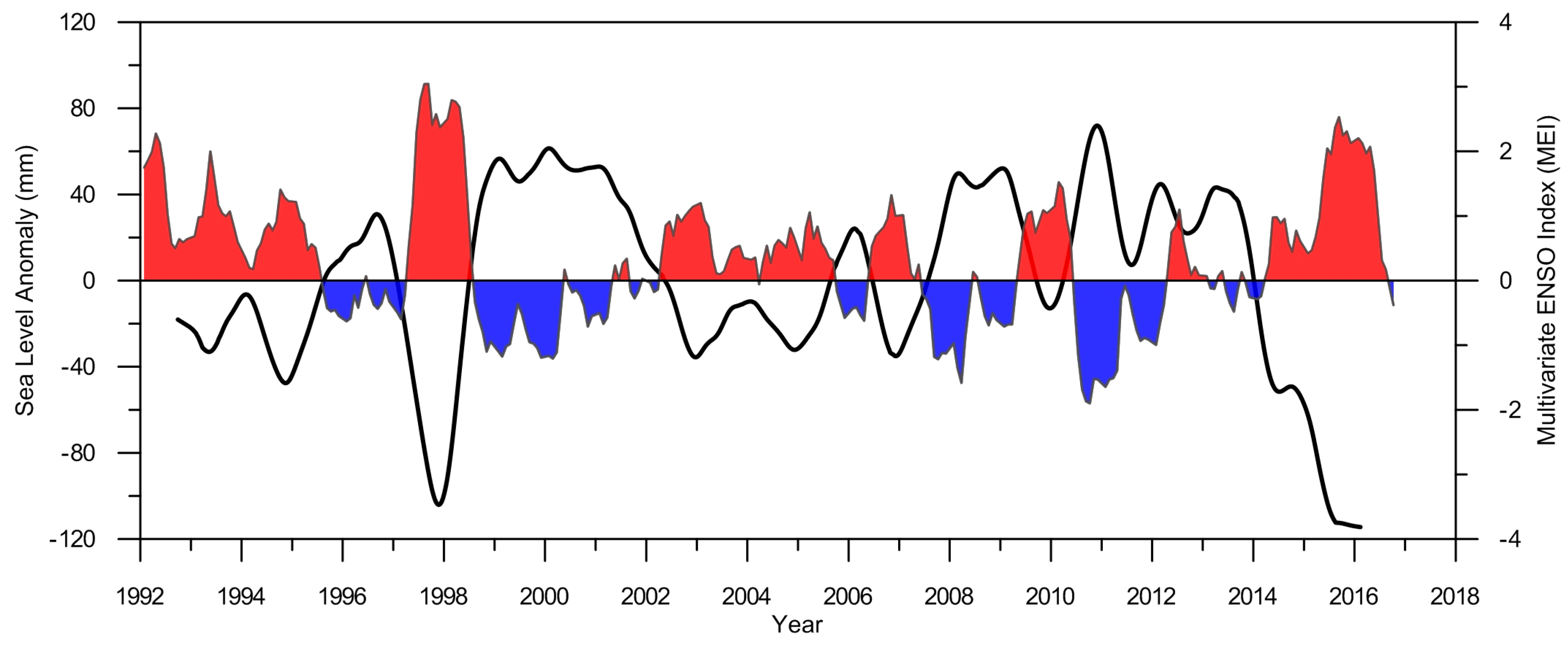Figure 26 shows the detrended SLA around the Indonesian seas overlaid with the Multivariate ENSO Index (MEI). The El Niño periods are indicated in red while La Niña periods are shown in blue. The striking feature of this figure is a perfect match of the periods when SLA is positive with those when MEI is negative and of the periods when SLA is negative with those when MEI is positive.

The ENSO event appeared around the Indonesian seas in several periods, but the strongest El Niño was during 1997–1998 and the strongest La Niña was in 2011. Another noticeable feature of the inter-annual variability seen in Figure 22 is the strong decrease in sea level since 2013, associated with the most recent El Niño.

In addition, the Indonesian seas have correlated behaviour with the surrounding seas, mainly from the South China Sea (SCS) [75]. The fresh and low-saline water from SCS flows into the Indonesian seas through the Java Sea to the Indian Ocean. The SCS water also flows through the Luzon strait to the Makasar strait and thus can influence the variability of ITF [76].

5. Conclusions

In this study, the assessment of various range and geophysical corrections and mean sea surface models has been performed for the Indonesia seas using TOPEX/Poseidon, Jason-1 and Jason-2 data for a period of 23 years. Table 3 shows the selected set for the various range and geophysical corrections and mean sea surface models, which were used to estimate the SLA time series for this region.

In summary, the best choice and adopted models for the range corrections are, for all missions: the ERA-Interim model for the dry tropospheric correction, the wet tropospheric correction from the GNSS-derived Path Delay algorithm and the smoothed dual-frequency ionospheric correction; the parametric sea state bias (SSB) BM4 model for TOPEX-A and Poseidon, the non-parametric-CLS model for TOPEX-B; the Tran2012 model for Jason-1 and Jason-2. Regarding the geophysical effects, the ocean tide FES2012 shows the best performance in the coastal area up to 60 km while GOT4.10 evidences the best overall performance in the open ocean. The CNESCLS_2011 mean sea surface model was adopted for all missions due to the SLA variance reduction this model causes, particularly in the coastal band up to about 40 km from the coast, when compared with DTU13 MSS.

Using the selected set of corrections and models, the sea level trend in the Indonesia seas has been estimated as 4.2 ± 0.2 mm/year over the 23 years of the altimetric period (1993–2015). If glacial isostatic adjustment (GIA) (0.3 mm/year) is applied, sea level rise is 4.5 mm/year. The rate of sea level rise in this region, derived from altimeter missions over 23 years is higher than the global mean sea level rate about 3.2–3.3 mm/year [13,14]. The positive values of sea level trend in this study are about 2–7 mm/year in agreement with other results in the same areas using altimetry [18,19,20]. The variability of sea level around the Indonesia seas is high mainly due to the effect of ENSO event (El Niño/La Niña). Due to the strong inter-annual signal, we show that the sea level trend in this region is very sensitive to the time span used in the analysis and to the set of adopted corrections. We show that the detrended SLA time series for the Indonesia region has a strong negative correlation (–0.79) with the Multivariate ENSO Index (MEI).

In this study, the sea level rate has been deduced only from satellite altimetry data. Complementary and relevant information on sea level variation can be derived from tide gauge data. However, due to the instability of the region, tide gauge measurements are often not reliable. Moreover, when analysing tide gauge data, the vertical movement caused by tectonic and volcanic activities and anthropogenic subsidence directly affects the tide gauge measurements. For example, Jakarta, the capital of Indonesia, has subsidence rates about 3–10 mm/year for the period 1974 to 2010 [77] and sea level rise derived by tide gauge time series measurement and satellite altimetry for periods 1993 to 2009 are about 23 mm/year and 3.8 mm/year, respectively [18]. For the future work, due to the high seismic activity around Indonesia, the analysis of altimetry, tide gauge measurement and information of vertical motion can be expected to better characterise the actual sea level change in the Indonesian region, particularly at coastal areas.