Article

Atmospheric Profile Retrieval Algorithm for Next Generation Geostationary Satellite of Korea and Its Application to the Advanced Himawari Imager

1
Department of Atmospheric Sciences and Engineering, Ewha Womans University, 52, Ewhayeodae-gil, Seodaemun-gu, Seoul 03760, Korea
2
National Meteorological Satellite Center, 64-18, Guam-gil, Gwanghyewon-myeon, Jincheon-gun, Chungcheongbuk-do 27803, Korea
*
Author to whom correspondence should be addressed.
Remote Sens. 2017, 9(12), 1294; https://doi.org/10.3390/rs9121294
Submission received: 25 October 2017 / Revised: 5 December 2017 / Accepted: 8 December 2017 / Published: 12 December 2017
(This article belongs to the Section Atmospheric Remote Sensing)

Abstract

:
In preparation for the 2nd geostationary multi-purpose satellite of Korea with a 16-channel Advanced Meteorological Imager; an algorithm has been developed to retrieve clear-sky vertical profiles of temperature (T) and humidity (Q) based on a nonlinear optimal estimation method. The performance and characteristics of the algorithm have been evaluated using the measured data of the Advanced Himawari Imager (AHI) on board the Himawari-8 of Japan, launched in 2014. Constraints for the optimal estimation solution are provided by the forecasted T and Q profiles from a global numerical weather prediction model and their error covariance. Although the information contents for temperature is quite low due to the limited number of channels used in the retrieval; the study reveals that useful moisture information (2~3 degrees of freedom for signal) is provided from the three water vapor channels; contributing to the increase in the moisture retrieval accuracy upon the model forecast. The improvements are consistent throughout the tropospheric atmosphere with almost zero mean bias and 9% (relative humidity) of root mean square error between 100 and 1000 hPa when compared with the quality-controlled radiosonde data from 2016 August.

Graphical Abstract

1. Introduction

Timely information on the vertical distribution of temperature (T) and moisture (Q) is critical to the prediction of weather phenomena. Particularly severe weather events associated with a thermodynamically unstable atmosphere are hard to predict since they are related with rapidly developing convective systems in short time period with small scale that most operational models cannot resolve [1]. Thus, it is important to have atmospheric profile information with high spatial resolution in a timely manner. Although such atmospheric information is provided through prediction or measurement from Numerical Weather Prediction (NWP) models or hyper-spectral sounders onboard polar orbiters, both are provided in lower temporal and spatial resolution compared to that from the next generation high-performance geostationary imagers such as the operational Advanced Himawari Imager (AHI) on board the Himawari-8, Advanced Baseline Imager (ABI) on board the Geostationary Operational Environmental Satellite-R (GOES-R) series, or the planned Advanced Meteorological Imager (AMI) on board the Geostationary Korea multipurpose Satellite-2A (GK-2A). Furthermore, the accuracy of NWP models, which greatly depends on the initial condition [2], decreases in the presence of clouds or in data sparse regions. In contrast, the new imagers, have, or will have the capabilities to monitor the evolution of convective clouds from the pre-convective stage with a fast scanning rate (about 10 min for the full-earth disk and much shorter interval for limited areas) and a finer spatial resolution (2 km for infrared channels).
In addition to the improved spatial and temporal resolution, the increased spectral capacity (Table 1) of the imagers suggests possibility of sounding retrieval. Retrieval simulations and theoretical analysis [3] showed that ABI data, in conjunction with NWP model forecast information, may produce additional moisture information that can improve forecast and will be able to adequately substitute legacy sounder-based products. Jin et al. [4] also showed that useful water vapor information in the upper layer (higher than 700 hPa) can be derived from the Spinning Enhanced Visible and Infrared Imager (SEVIRI) and simulated ABI data with high spatial and temporal resolution using the ABI Legacy Atmospheric Profile (LAP) retrieval algorithm, which was originally developed for GOES Sounder products [5] based on an iterative physical retrieval scheme. Lee et al. [6] applied the same retrieval scheme to the GOES-13 sounder measurements and evaluated the moisture-related products such as total precipitable water (TPW) and lifted index including vertical profiles of temperature and moisture. The results showed that the retrieved moisture (relative humidity) profile significantly improves upon the Global Forecasting System (GFS) forecast from National Centers for Environmental Prediction (NCEP) between 300 and 700 hPa while the retrieved temperature profile shows similar accuracy to the model forecast field when compared with radiosonde measurements.
The new imager of Korea, AMI, will improve upon the current meteorological imager (MI) with four times finer spatial resolution (from 4 km to 2 km for infrared (IR)), five times reduced time latency (from 27 min to less than 5 min to scan the full earth’s disk) and increased spectral capacity (4 visible (VIS), 2 near-IR (NIR) and 10 IR) [7]. With the improved capability of AMI, it is expected that not only the measured radiance but also retrieved or derived information such as vertical profiles of temperature and moisture, TPW, or atmospheric instability indices provide additional useful information to weather forecasters in nowcasting or short-range severe weather forecasting. In preparation for GK-2A, an algorithm has been developed for the retrieval of clear-sky vertical profiles of T and Q from the measured radiance of AMI based on an iterative nonlinear optimal estimation method [8,9,10]. Unlike previous studies, which theoretically showed the potential usefulness of information retrieved from pseudo- or simulated ABI data, the algorithm developed in this study employs real-time measurements from AHI, which has very similar spectral specification with AMI, in terms of the number of infrared channels and central wavelength. To ensure the retrieval accuracy, AHI radiance is calibrated with a simple bias correction process and analyzed for characterization of the algorithm. A priori constraints to the solution is given by the forecast fields produced from the Korean Meteorology Agency (KMA) global prediction model, which is based on the UK Met-Office Unified Model (UM). Unlike previous studies, which used a regression technique for the generation of first-guess fields by combining the simulated brightness temperature (TB) of ABI with the GFS forecasts [5] or the simulated GOES-13 sounder TB with the NCEP forecast fields [6], the study directly employs the forecasts without using regression. The main reason for using a regression as the first guess is to improve the retrieval accuracy by combining model forecasts with the measurements as predictors [11]. However, it requires great computational efforts and periodic monitoring and updates of the regression coefficients. In addition, the accuracy of NWP model forecasts has been increasing, which makes it possible for the retrieval process to converge to a solution fast with a first guess that is directly taken from the model forecast as is the case in this study.
Algorithm products include vertical profiles of T, Q and ozone (O3) and derived atmospheric parameters such as TPW, total column ozone and atmospheric stability indices including K-index, Lifted index, Showalter index, Total totals and Convective Available Potential Energy (CAPE). Among the products, only the results for the retrieved profiles and TPW are presented in this paper. Starting from the description on the retrieval scheme, Section 2 provides the descriptions on the dataset used in the algorithm and experiments performed to improve the quality of dataset. Section 3 presents algorithm characterization and validation results and the summary and conclusion is provided in Section 4.

2. Data and Methods

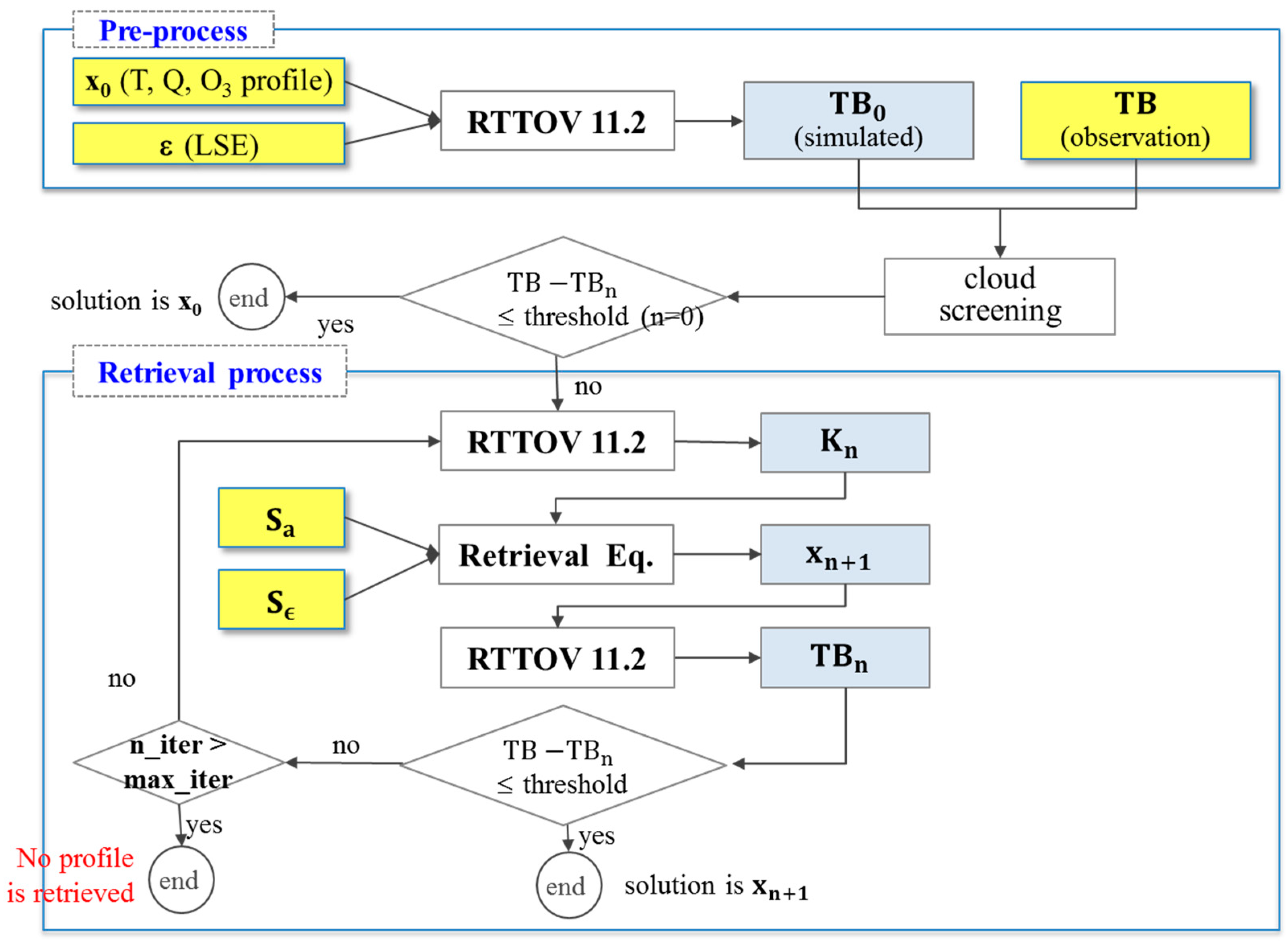
2.1. Retrieval Method

Determining continuous atmospheric profiles from a limited number of measurements is an inverse and ill-posed problem in that no unique solution exists. Therefore, to make the problem well-posed, one needs constraints to the solution by introducing additional information, which is called a priori constraints, background, or virtual measurements typically obtained from climatological mean profile with regression [12] or NWP model forecast with high accuracy without regression. This additional information combines with the satellite observations to determine the best profile from all the possible ones. One widely used theory to provide a method to this for a moderately nonlinear retrieval problem is optimal estimation [8,10]. This approach assumes that the errors associated with the observation and background are known and normally distributed (i.e., Gaussian). In order to find a best estimate of true profile x that maximizes the probability density functions of x given measurement (y), i.e., P ( x | y ) , the Bayes’ theorem is introduced to yield Equation (1),
2 ln P ( x | y ) = [ y F ( x ) ] T S ϵ 1   [ y F ( x ) ] + [ x x a ] T   S a 1   [ x x a ] + c
where x a is a state vector for background profiles, F is a forward model, S a and S ϵ represent error covariance matrix for background and observation, respectively and the superscript ‘T’ and ‘−1’ denote the transpose and inverse of a matrix, respectively. The right-hand side term is also known as the cost function [12] which needs to be minimized. This Bayesian optimal estimation solution [10] is a quadratic form in x, so the derivative of Equation (1) is equated to zero to find a state x ^ that makes the P ( x | y ) maximum or that makes the cost function minimum. Since the equation cannot be solved analytically, the Gauss-Newton method [10] is introduced to iteratively solve the equation. By ignoring small residuals, i.e., the first derivative of the Jacobians x K T , where K ( x ) = x F ( x ) , an iterative solution is obtained as follows:
x n + 1 = x 0 + S a K n T   ( K n S a K n T + S ϵ ) 1 ( TB TB n + K n × ( x n x 0 ) )
In this equation, the best estimate of the state ( x n + 1 ), composed of temperature, humidity and ozone profiles and surface skin temperature, is obtained by iterative updates on the background profile x 0 ( x a in Equation (1)). The gain matrix, S a K n T   ( K n   S a   K n T + S ϵ ) 1 , maps measurement space into state space, thereby propagating errors in measurements into the retrieved state. Also, S a and S ϵ determines or gives a balance between the amount of contribution that the background or the observations make for the retrieval and thus it is important to have as realistic and accurate error matrices as possible for both S a and S ϵ in a retrieval process.
The overall algorithm flow for the clear-sky atmospheric profile retrieval is illustrated in Figure 1. The data pre-processing procedure includes the preparation and interpolation of input data for the radiative transfer model (RTM) simulation of TB which, in turn, will be compared with the observations. Before the comparison is made, AHI radiance is corrected using pre-calculated correction coefficients and then converted to TB. Detailed descriptions on data pre-processing including bias correction are given in Section 2.2. The background clear-sky TB is simulated using the Radiative Transfer for TOVs (RTTOV) version 11.2 [13] and compared with the observed TB averaged over cloud-free pixels within a processing unit, which can be either an individual pixel or a group of pixels (M × M FOV, 1 FOV = 2 km). For the identification of cloud-free pixels, the GK-2A cloud-mask product is used and a processing unit is determined as ‘cloud-free’ only if more than half the pixels in the unit are identified as cloud-free. Once the processing unit is identified as cloud-free, the mean AHI TB is compared to the simulated TB at the nearest model grid-point. If the difference between the two TBs is less than the pre-defined threshold for all channels used in the algorithm, the first-guess profile is taken as the solution and if not, the iterative retrieval process starts using the Equation (2) to adjust the first-guess profile until the difference gets smaller enough to meet the threshold. The threshold for convergence is defined as the observation error (see Section 2.2.4 for details) and the retrieval process repeats until it reaches the maximum number of iterations, i.e., 6. If the criterion is never met within 6 iterations, no profiles are retrieved.

2.2. Data

2.2.1. Satellite Measurements

The study applies the algorithm to measurements from Himawari-8 AHI which has very similar spectral configuration to that of AMI as shown in Table 1. In addition, positioned at 140.7°E, Himawari-8 scans the areas that will be included in AMI scan coverage. Therefore, using AHI for the algorithm will help a fast conversion from AHI to AMI upon the availability of AMI data. The algorithm uses 9 infrared channels (8 to 16) of AHI, among which channel 11 is used only for the retrieval over the ocean due to its large surface emissivity uncertainty over desert pixels [11].
In order to employ AHI data in the retrieval process, any systematic bias in the radiance field needs to be characterized and removed beforehand. Reference candidates for bias correction include radiances from a well-calibrated satellite instrument, NWP model background or analysis, collocated radiosonde and model fields generated near radiosonde stations [14]. In a previous study that applied the clear-sky ABI legacy profile retrieval algorithm to the SEVIRI measurements, Jin et al. [4] used quality-controlled radiosonde data for the bias correction of SEVIRI data and obtained significantly improved moisture retrieval accuracy in the upper atmospheric layers (600~300 hPa). In this study, two different reference data is used for a rough estimate of AHI bias on land and the ocean: the collocated one-month radiosonde (RAOB) data from June 2016 for the bias correction on land and the collocated 6-hourly ECMWF Reanalysis (ERA) data (00, 06, 12 and 18 UTC) from 1 to 10 June 2016 over the ocean. Upwelling radiance at the top of the atmosphere is simulated with RTTOV v11.2 and cloud-contaminated pixels are filtered out using the GK-2A cloud-mask. The simulated radiance is compared with the AHI radiance to get the fitting coefficients C0 (y-intercept) and C1 (slope) for the land and the ocean, separately. Figure 2 shows the departures of the simulated TB with ERA over the ocean (Figure 2a) and RAOB on land (Figure 2b) from the observations. As can be seen in the figures, AHI water vapor channels 8, 9 and 10 show positive bias over the ocean, while longer infrared channels show negative bias compared to the simulated ERA TB. This result is very similar to the patterns shown in the previous study [15] using RTTOV v11.2 with the ECMWF analyses. Over the land, on the other hand, AHI TB shows negative bias with respect to the simulated RAOB TB for all channels.
Introducing the method suggested by Hewison et al. [16] to estimate the relationship between radiances from two different instruments (Equation (3)), two sets of fitting coefficients are obtained from the comparison results and applied to AHI radiance to remove, if any, systematic bias
Radiance ( AHI ) = C 0 + C 1 × Radiance ( reference ) Radiance ( AHI bias corrected ) = ( Radiance ( AHI ) C 0 ) / C 1
After the bias correction, the retrieval accuracy of moisture profile (both bias and the root mean square error (RMSE)) is improved throughout the atmospheric layers, particularly in the mid to upper layers between 800 and 200 hPa as shown in Figure 3. In addition, before the bias correction, the retrieval shows very little or no improvement over the forecast, while the improvements are visible after the bias correction, indicating the importance of bias correction of measurements in a retrieval process.

2.2.2. First Guess Profile

In the study, the algorithm uses global forecast fields (t + 6 to t + 11 with 1-h interval) from UM-based global prediction model of KMA as its first guess. The model resolution is 0.234° in longitude by 0.156° in latitude (about 17 km) up to 80 km. The first guess from the model forecasts includes surface skin T, surface pressure, 2m-T, 2m-Q and profiles of T and Q (mixing ratio) on the model layers, which is interpolated to the RTTOV 54 pressure levels. Spatially, the model grid point nearest to the center of AHI pixel (3 × 3 FOVs in this study) is selected and temporally, two neighboring forecast fields (e.g., 6-h and 7-h forecast fields) are read-in and interpolated to the AHI scene between the hours (e.g., 0610 UTC).
Meanwhile, ozone forecast is not produced from UM and thus the first guess profile for ozone is created using a monthly ozone climatology [17] and Level 2 total column ozone derived from the Ozone Monitoring Instrument (OMI) passing over the area of interest between 00 and 10 UTC on the previous day. The ozone climatology is merged data from 22 years of balloon sonde (1988–2010) and Aura Microwave Limb Sounder (2004–2010) measurements for 18 latitudinal bands (10-degree intervals) covering from 0 to 65 km altitudes. The low spatial and temporal resolution of the ozone climatology becomes the main source of failure in the retrieved total column ozone capturing the latitudinal variability in the mid-latitude and of the apparent discontinuities between latitudinal bands shown in the retrievals. For this reason, the study employs near real-time measurement, i.e., the day-1 OMI total ozone, the distribution of which does not change significantly in one day. The OMI total ozone is utilized to determine the most appropriate climatological ozone profile that can best describe the distribution of the near-real time total ozone field among all the profiles. More detailed descriptions on this process are given by Ha et al. [18]. Improving the ozone first-guess by selecting the climatological profile that is the most relevant to the previous-day total ozone measurements contributes to decrease the bias in the mid-latitudes and to lessen the latitudinal discontinuities shown in the retrieved total ozone.
All the variables, except the 2m-T, 2m-Q and surface pressure, are updated at each iteration step in the retrieval process.

2.2.3. Background Error Covariance

An accurate specification of background error covariance is important not only for successful data assimilations [19] but also for accurate retrievals since it decides the weights given to the observation and the first-guess field thereby changing the increment and eventually the retrieval accuracy. The background error covariance matrix (B-matrix) currently applied to the algorithm, denoted S a in Equations (1) and (2), is a 163 by 163 matrix including error covariance sub-matrices for T (54 by 54), Q (54 by 54) and O3 (54 by 54) and the error covariance for surface skin temperature of the background. The T and Q error covariance are obtained from KMA Observation Pre-processing System (OPS) and they are provided for three latitudinal bands, i.e., 90°S to 30°S, 30°S to 30°N and 30°N to 90°N, with 43 pressure levels for T and 26 levels (surface to about 100 hPa) for Q. Since AHI measurements do not have humidity information above 100 hPa, the error covariance values for Q above this level are set to very small values and both T and Q error covariance are interpolated to the RTTOV 54 pressure levels. The background error covariance for ozone, which is not produced from UM, is obtained from ECMWF one-dimensional variational (1DVar) system.
To see the impact of B-matrix on the retrieval, a sensitivity test was performed with differently scaled B-matrix. In this test, the two terms in the inverse-weight in Equation (2), i.e., B-matrix ( S a ) converted to observation space ( K n S a K n T ) and the observation error covariance ( S ϵ ) are compared. Both have the same dimensions of nch by nch where nch is the number of channels used for the retrieval. If one term is too large compared to the other, the effect of the term with smaller value will be ignored in the retrieval process and thus both terms need to be in balance to some degree. As shown in Figure 4a, when the B-matrix of T is scaled by 0.01 to 100 with fixed Q error covariance, KS a K T shows very little change. On the other hand, as shown in Figure 4b, KS a K T in water vapor channels dramatically change with varying B-matrix of Q. In other words, KS a K T is much more sensitive to the change in the Q error covariance than in T and this change is more prominent in the water vapor channels (Ch. 8–10) than in the window (Ch. 13–15) or CO2 absorption (Ch. 16) channels. This implies that if mis-scaled S a is used and the magnitude of KS a K T is not balanced out with S ϵ in Equation (2), the weight given to the satellite measurement becomes too large or small, which may prevent the convergence to the optimal solution.

2.2.4. Observation Error Covariance

Observation error covariance matrix denoted S ϵ in Equations (1) and (2) is a square matrix of order 9, i.e., the number of AHI infrared channels used in the study. The off-diagonal components of the matrix are all set to zero and the diagonal components are given by the sum of the variance of measurement errors (or instrument noise) and forward model uncertainty (0.2 K). Since the correlations between two different channels (i.e., off-diagonal components) are ignored, to compensate this, the measurement error variance is scaled by an inflation factor [20] of 3. For the instrument noise, the algorithm introduces the Noise Equivalent differential Temperature (NEdT) corresponding to each infrared channel of AHI. NEdT is calculated from the Noise Equivalent differential Radiance (NEdR) using the Planck function. Unlike NEdR, which can be directly calculated in a controlled environment for each channel and thus independent of the target scene temperature, NEdT depends on the scene temperature with a smaller value for a warm scene and a larger value for a cold scene. Therefore, in order to use NEdT as a representative noise measure of an instrument in a retrieval process, NEdT needs to be dynamically assigned according to the scene temperature of a target to be retrieved. If the number of target clear pixels is n c l r and the NEdT of channel ich corresponding to the target mean TB is NEdT i c h , then the diagonal components of the observation error covariance matrix S ϵ can be expressed as:
S ϵ ( i c h , i c h ) = ( NEdT i c h n c l r × ( inflation   factor ) ) 2 + 0.2 2

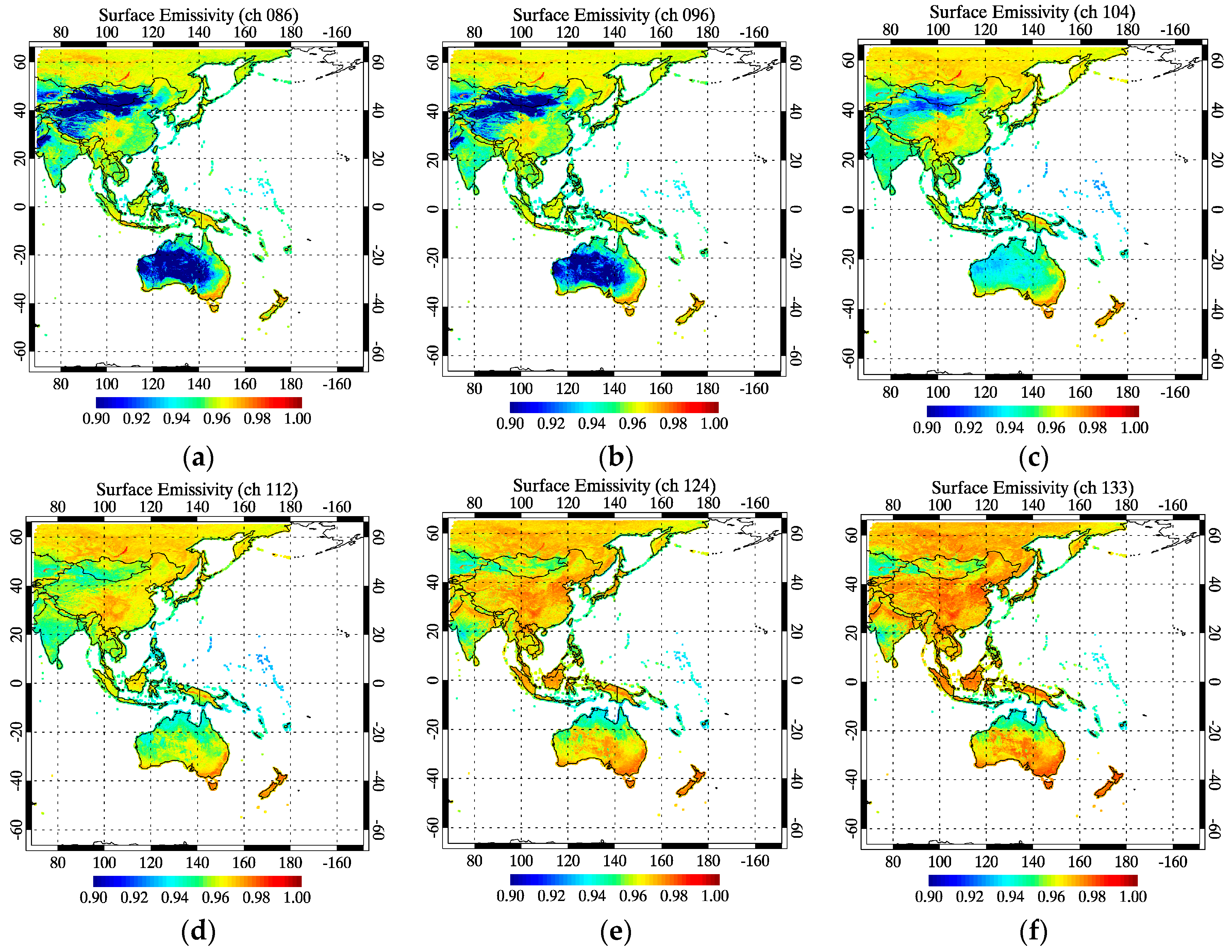
2.2.5. Land Surface Emissivity

Using an accurate land surface emissivity (LSE) data is essential for the simulation of accurate brightness temperature, particularly for the channels sensitive to the surface. For example, 1% emissivity error in the window channels may result in TB changes of about 0.5 K [11]. Accurate LSE is critical not only for the assimilation of satellite radiances in NWP models on land but also for the retrieval of atmospheric profiles of temperature and moisture along with the surface skin temperature [21,22]. Currently, available accurate data is the global infrared monthly LSE database developed at the Cooperative Institute of Meteorological Satellite Studies (CIMSS) using the baseline fit method [23]. The database is generated based on the operational MODerate resolution Imaging Spectroradiometer (MODIS) surface emissivity product and is provided at ten wavelengths (3.6, 4.3, 5.0, 5.8, 7.6, 8.3, 9.3, 10.8, 12.1 and 14.3 μm) with 0.05° grid intervals. To provide stable LSE data for the real-time retrieval, using a monthly climatological emissivity data can be an alternative. Thus, a monthly climatological emissivity data was created from the twelve years (from 2003 to 2014) of CIMSS emissivity database. Although the database shows relatively large inter-annual variation of about 0.05 in channel 12.1 and 14.3 μm, particularly during the summer months and in September between 2006 and 2007, overall variation is smaller than 1% (0.01). Then the created climatological data is then interpolated to the ten infrared channels of AHI using Akima Spline method. Figure 5 shows the created climatological LSE data for the channels 8.6, 9.6, 10.4, 11.2, 12.4 and 13.3 μm.
Meanwhile, the emissivity values for the five days at the beginning and at the end of each month are calculated using linear interpolation to remove discontinuities between months, which are relatively large between December and January and between March and April, showing the largest difference for channel 8.6 μm in arid areas in East Asia. The algorithm limits the use of channel 8.6 only for the ocean but the interpolation between two months leads to a more accurate RTM simulation by minimizing the inter-month discontinuities in the window channels as well.

2.3. Summary

This section summarizes the algorithm specification described in Section 2.1 and Section 2.2. A clear-sky atmospheric profile retrieval algorithm, originally developed for the profile retrieval from AMI, is applied to AHI measurements from 9 infrared channels as shown in Table 2. Based on the Bayesian optimal estimation method, the algorithm iteratively updates the first-guess profile until the convergence threshold is met. The first guess profiles for temperature and moisture are obtained from the KMA UM 6 to 11 h forecasts and the ozone first guess profile is created by interpolating the monthly ozone climatology using OMI total ozone measured the previous day. The errors in the measurements and the background are given as respective error covariance matrix, S ϵ and S a . LSE data required for the TB simulation is monthly climatological data, created based on twelve years of CIMSS global infrared LSE database, which is interpolated to AHI infrared channels. For the TB simulation and the calculation of Jacobians, RTTOV version 11.2 is used.

3. Results

3.1. Algorithm Characterization

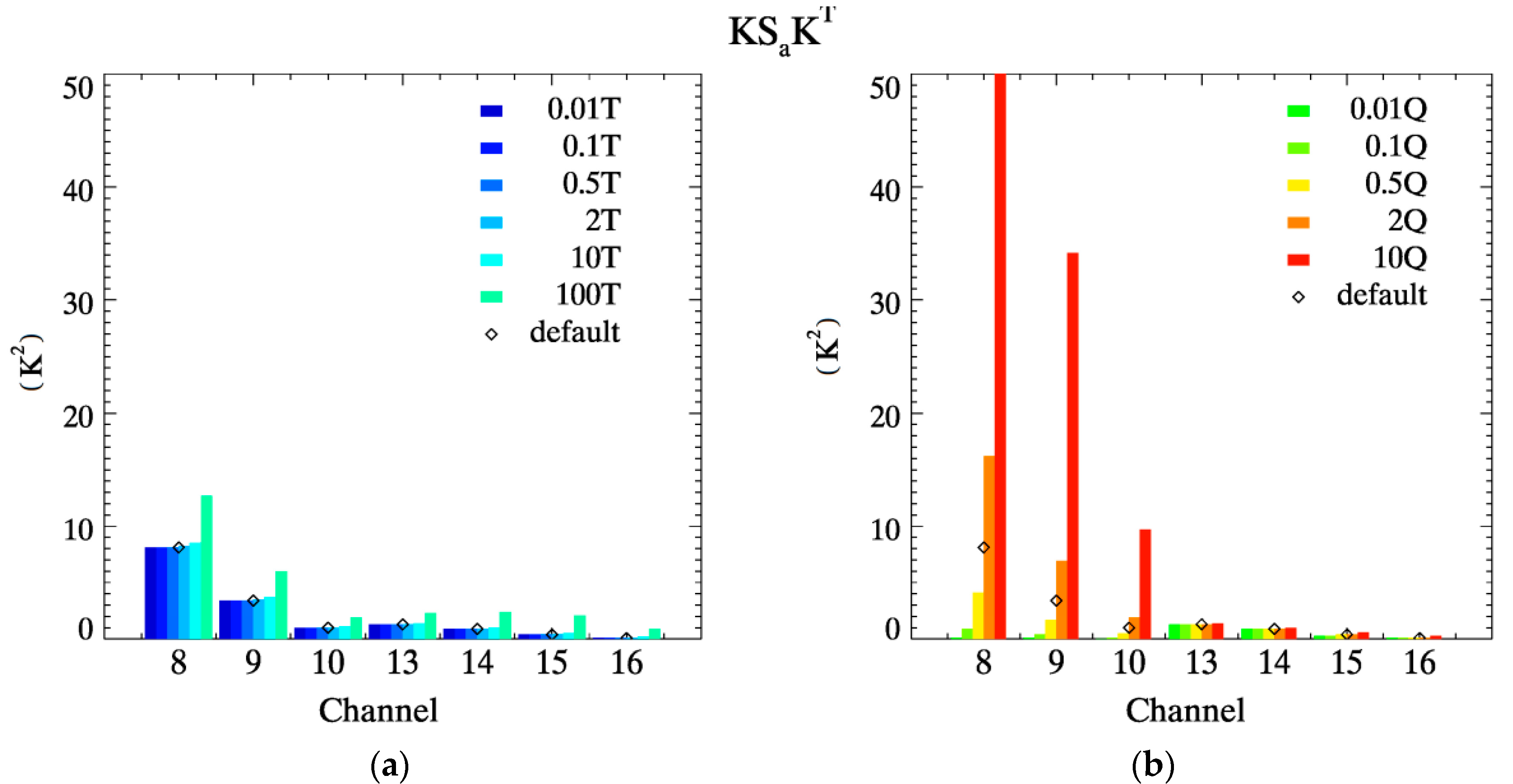
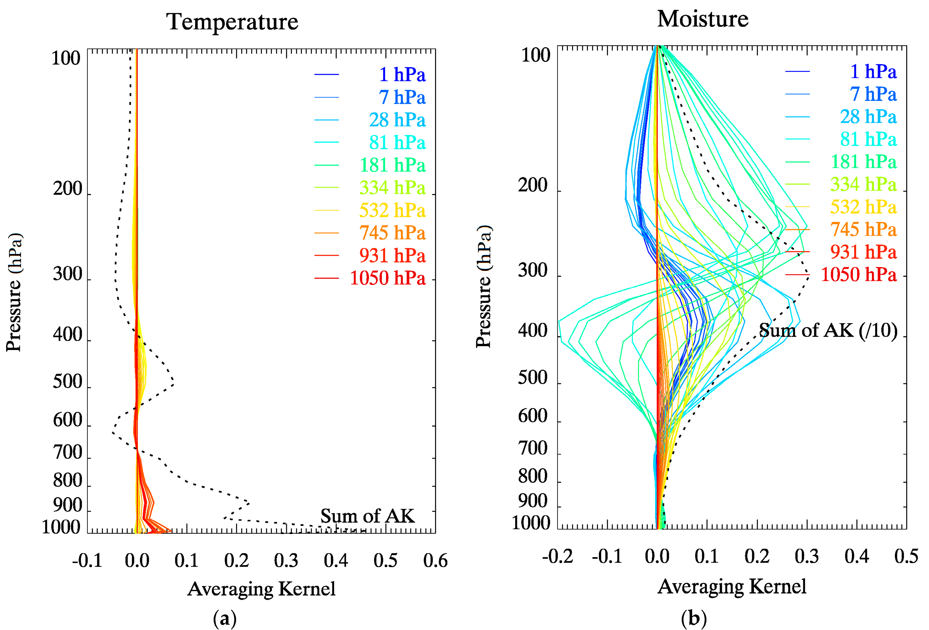
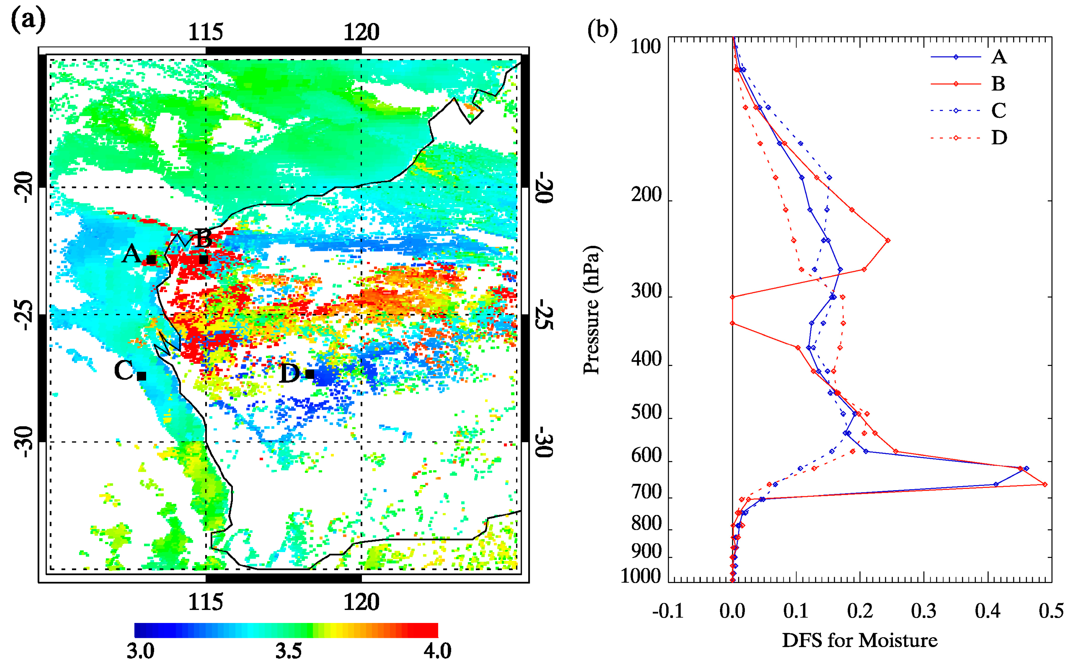
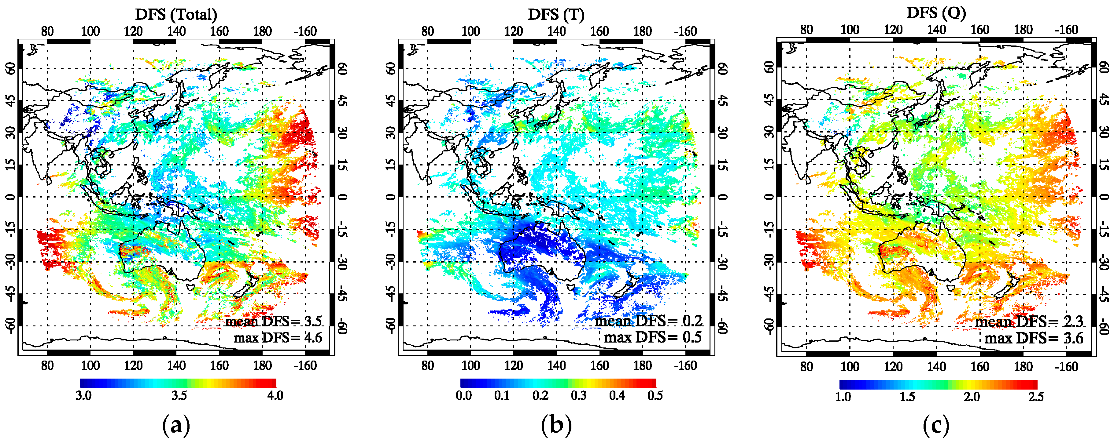
3.1.1. Information Contents of Measurements

A measure to evaluate the information contents of measurements is averaging kernels (AK), defined [10] as Equation (5). It is a measure of the amount of information coming from the measurements with respect to the information from the a priori [24]. Figure 6 shows AK evaluated at the final iteration of the retrieval process for temperature (Figure 6a) and moisture (Figure 6b) at a specific time and location over the ocean. The black dotted line in the figure indicates the area, or the sum of the rows, of AK and it is supposed to be about unity at levels where accurate retrieval is made [10]. The peak height of the AK area, which indicates the altitude where the tropospheric retrieval has maximum sensitivity to the change in the true state, is about 960 hPa for temperature and 300 hPa for moisture.
A = ( K i T   S ϵ 1   K + S a 1 ) 1   K i T   S ϵ 1   K i
d s =   tr ( A )
Another widely used measure for the amount of useful independent information in measurements is the degrees of freedom for signal (DFS) and it is calculated from the AK given [10] in Equation (6). Both AK and DFS vary depending on the scene temperature, surface pressure, or latitude and also mathematically depend on the error covariance terms. The dependence of DFS on the sun elevation angle, aerosol optical depth and vegetation type over land has also been investigated [25]. The influence of these various factors on DFS can be found in Figure 7, where the mean total DFS (Figure 7a) is given as the sum of DFS for the three retrieval parameters, i.e., T (Figure 7b), Q (Figure 7c) and O3. The most noticeable feature in the figures is that the distribution of total DFS is determined mostly by the distribution of DFS for Q, which is the largest (maximum 3.6 DFS) among the three parameters. The mean DFS for temperature is much smaller (approximately 0.3) than the moisture due to the lack of information in AHI measurements for temperature sounding and/or tightly constrained a priori error covariance. The distribution of DFS for O3, which is not presented here, shows almost little variation with constant DFS of about 1.0.
Since the algorithm employs additional information from channel 10 for the retrieval over the ocean, the DFS values over the ocean is higher than the DFS over land in general. The relatively high DFS values, particularly Q and total DFS, around the edges of the full-disk is related to the long path length, which increases the sensitivity of the TB at the top of the atmosphere to water vapor in the air (i.e., moisture Jacobians) and this in turn contributes to the increase in the DFS. The discontinuities shown in the three figures near the 30 degree south reflect the influence of the background error covariance term, S a on the DFS. As explained in Section 2.2.3, the covariance matrices are provided for three latitudinal bands, i.e., 90°S~30°S, 30°S~30°N and 30°N~90°N and the provided moisture error covariance values are relatively high in the 90°S~30°S latitude band than in the other two bands, which leads to the higher DFS in the southern hemisphere ocean below −30° latitude and the discontinuities between the latitudinal bands. Over land, the DFS shows high spatial variability, as can be seen in the magnified Figure 8a for the western part of Australia shown in Figure 7. To see where in the atmospheric layer the information contents contribute the most to the moisture DFS, the profiles of Q DFS (Figure 8b), i.e., diagonal elements of the AK, over land and ocean are compared. The solid lines indicate the DFS profiles with comparatively high total DFS over the ocean (A) and land (B), respectively, while the dotted lines are the DFS profiles with comparatively low total DFS over the ocean (C) and land (D), respectively. The corresponding locations are shown in Figure 8a. The DFS profiles show that regardless of the surface type, the retrieval sensitivity to water vapor is significantly high between 600 and 700 hPa layer, leading to the increase in the total DFS.

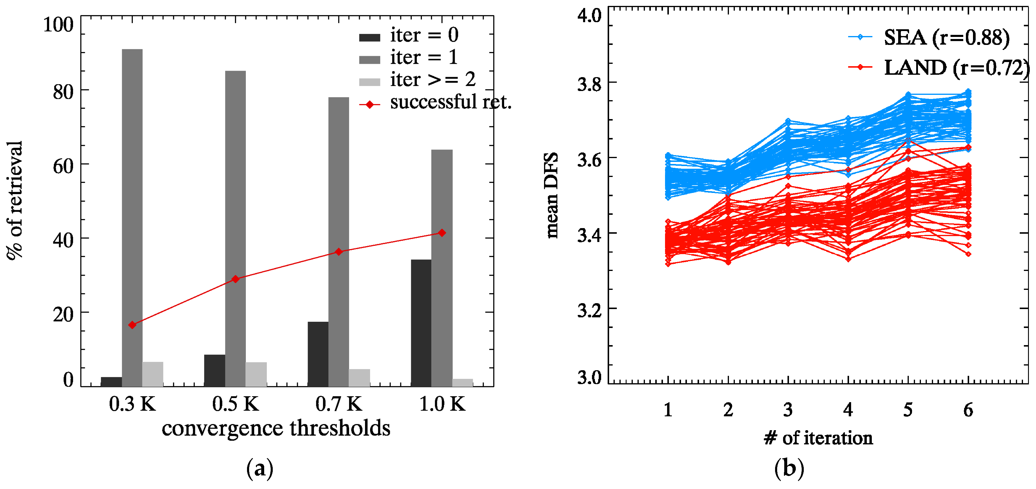
3.1.2. Convergence Threshold and Iteration

The threshold for convergence needs to be determined with care because it is directly related to the retrieval accuracy and at the same time to the successful retrieval rate of a scene. If the threshold is too tight, very little retrievals are achieved with higher retrieval accuracy and if it is too relaxed, profiles are retrieved from more pixels but with a degraded accuracy. The level of tightness of this convergence threshold also influences on the number of iterations required for the convergence. If the first guess is close enough to the observations within the pre-defined threshold, the algorithm does not start the iterative retrieval process but instead takes the first guess as the solution. On the other hand, more iterations are required for convergence if the gap between the measurements and the first-guess increases. As shown in Figure 9a, the number of clear-sky retrievals with zero iteration increases as the thresholds are relaxed from 0.3 K to 1.0 K and so thus the successful retrieval rate (red line), while more iterations are required with tighter thresholds. The results from one-month (August 2016) statistics show that the algorithm requires the iterative process for more than three fourths of the clear-sky retrievals with a rather relaxed threshold of 0.7 K but when the threshold is tight to the level of observation error, almost 99% of the retrievals are achieved by the iterative process.
Meanwhile, the relationship between the number of iterations and the information contents of the pixels to be retrieved is analyzed and the result reveals that pixels with higher information contents, or total DFS, go through more iteration to reach convergence as shown in Figure 9b. Each line in the figure indicates the mean total DFS on land (red) and ocean (blue) from a different scene in August 2016 and the figure shows that there is a positive correlation between the mean total DFS and the number of iterations required in the retrieval process. The correlation between the two is higher over the sea (r = 0.88) than on land (r = 0.72). Since the retrieval process requires more iterations when the gap between the first guess and the measurements is larger, the results can be interpreted as that the high information contents contributes to converge to a solution of the retrieval process, especially when the model forecast is far from the observation.

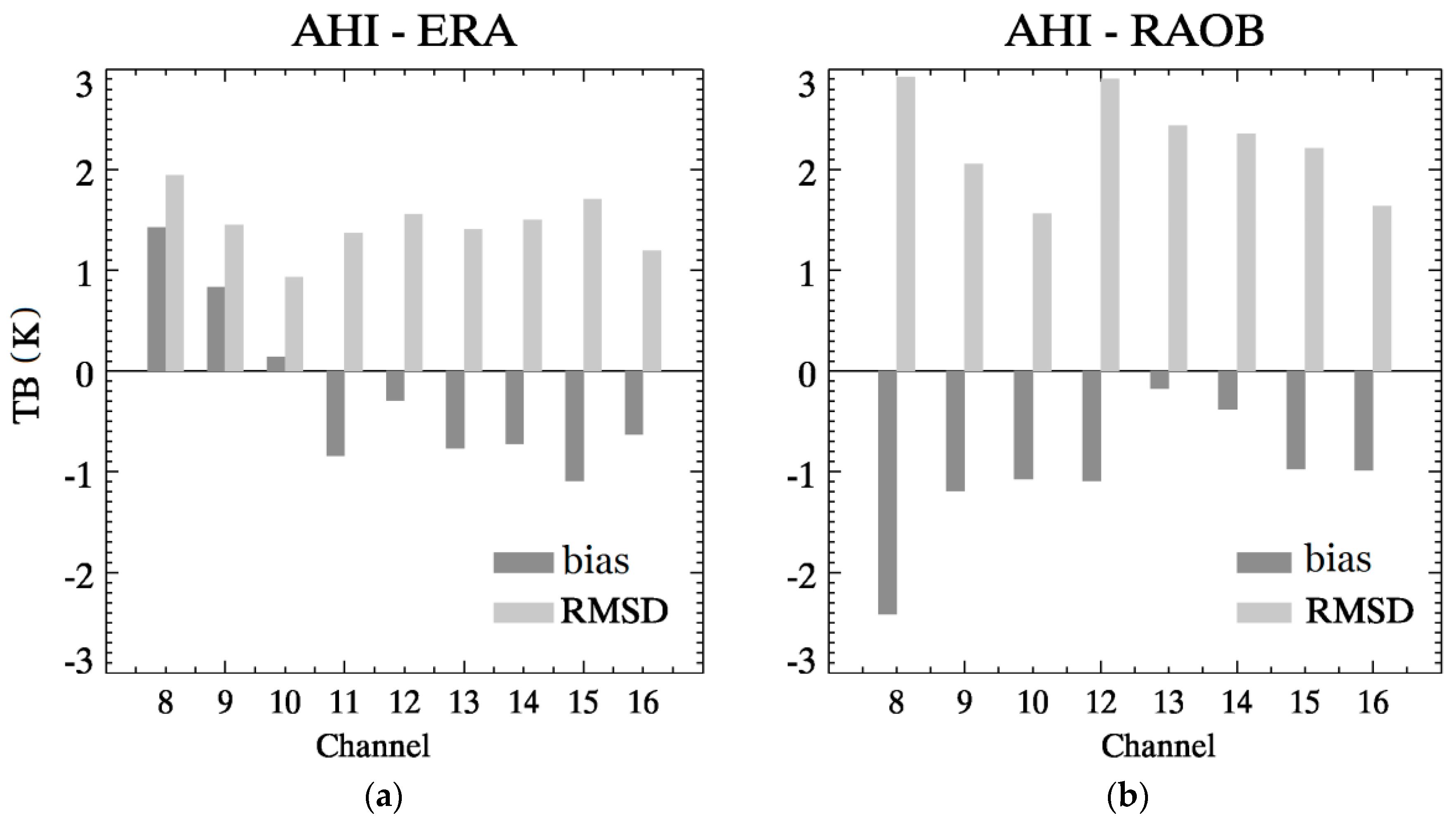
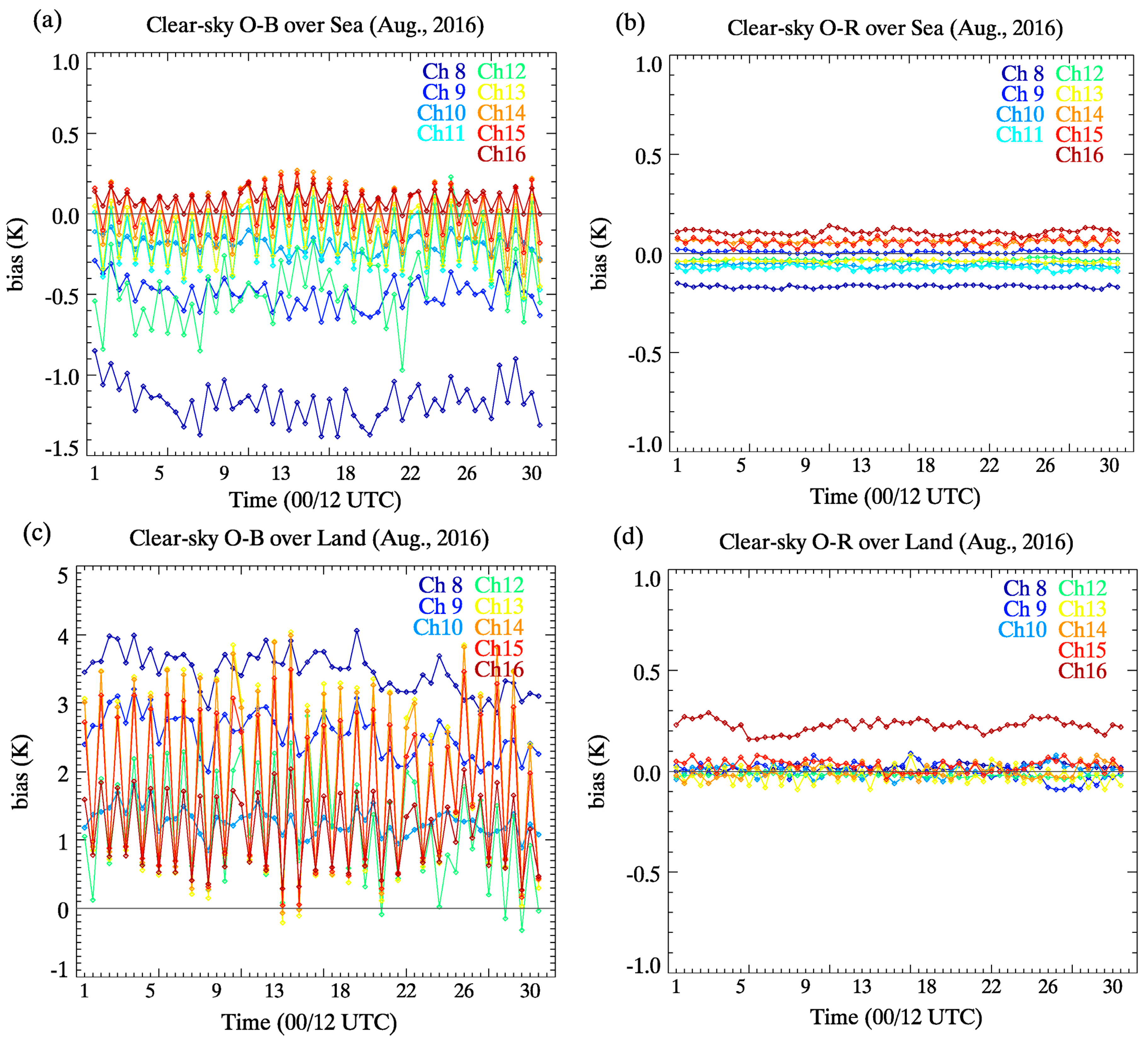
3.1.3. TB Departures

The difference between the bias-corrected observations and simulated TB before and after the retrieval, i.e., observation minus background (O-B) and observation minus retrieval (O-R), respectively, in the observation space were analyzed to see how much improvements are achieved over the first-guess with the retrieval process. One month data from August 2016 with 12-h intervals are used to analyze the time series of O-B and O-R for cloud-free pixels over the ocean and land. As shown in Figure 10a,c, O-B shows a diurnal variation in most of the channels with bigger fluctuations in the window channels on land. Over the ocean, the bias in the water vapor channels (particularly in channel 8 (6.2 μm)) is relatively large compared to other channels. The diurnal variation of O-B values in the surface-sensitive channels may be attributed to NWP model skin temperatures, which are not representative of the surface temperature but of a deeper layer and held fixed over the ocean during the day [13]. The diurnal variations shown in the water vapor channels, which are not sensitive to the surface nor to clouds, may also be attributed to NWP models which are known to have diurnal variations of humidity in the upper troposphere over convective regions and have the patterns that are substantially different from that of satellite observations [26,27,28]. After the retrieval (Figure 10b,d), however, the statistics are very stable with small bias within the observation error range throughout the analyzed time period. Over the ocean, the biggest adjustment on the first-guess is seen in the upper water vapor channel with significantly reduced diurnal variation, which leads to visible improvements in upper atmospheric moisture retrievals over the forecasts, as shown in the validation results (Section 3.2.1).

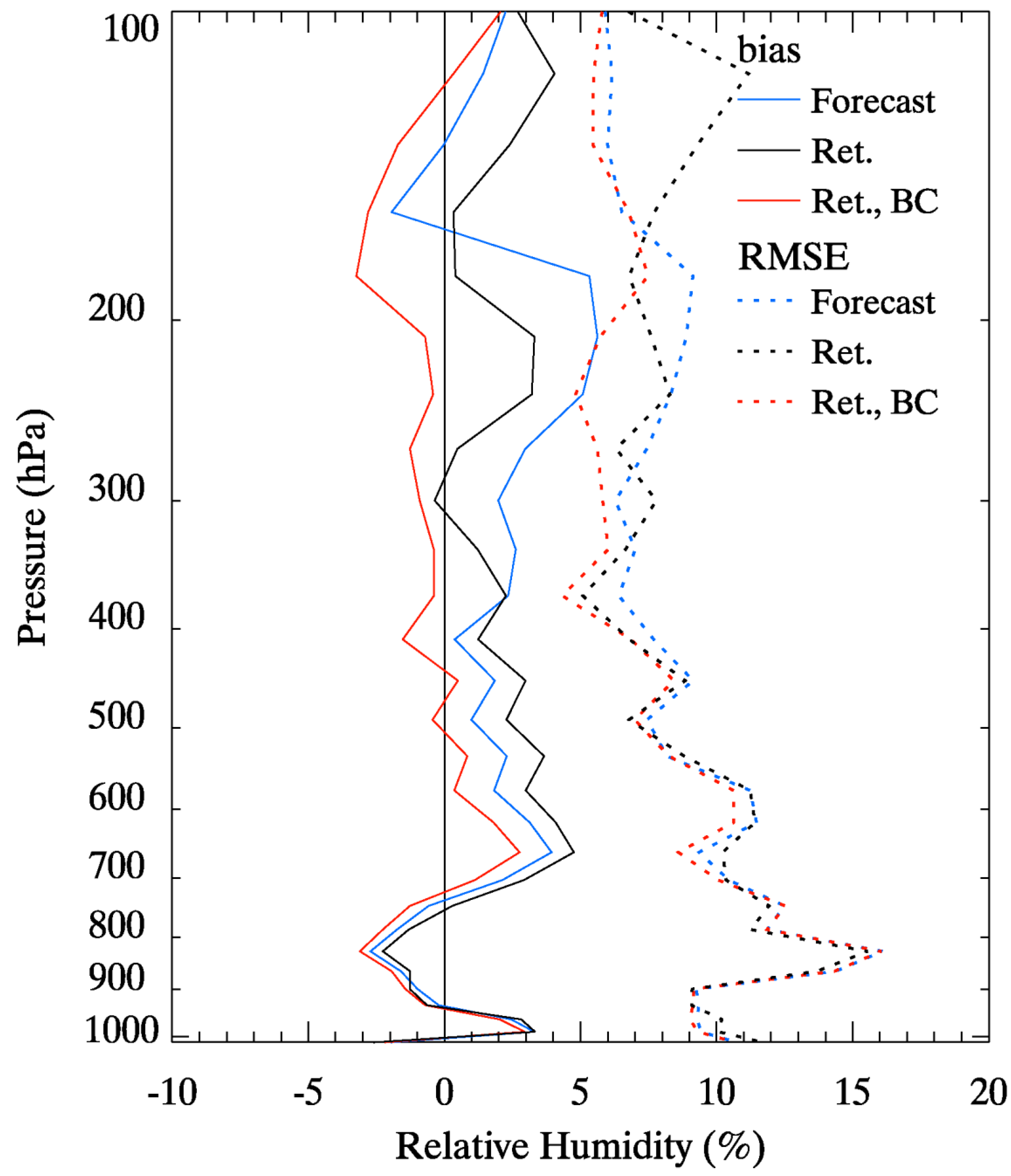
3.2. Validation Results

The focus of the validation in this study is on the moisture-related products to see how much useful information the three water vapor channels in AHI (or AMI) provide. For this, validation results for retrieved atmospheric profiles and TPW are presented together with the results for the integrated layer precipitable waters (LPW) for the three atmospheric layers, i.e., the surface and 850 hPa (LPW1), 850 and 400 hPa (LPW2) and 400 and 200 hPa (LPW3).
For the evaluation of the retrieval accuracy, a quality-controlled reference data such as radiosonde or reliable NWP model analysis is required. However, the accuracy of model analysis differs by operational centers depending on the models and quality control schemes that the centers employ for the assimilations [27]. In addition, the accuracy of radiosonde measurements greatly depends on radiosonde types and stations [29,30], which will, in turn, affect the accuracy of NWP models that employ radiosonde data for the assimilations. According to WMO technical reports on the accuracy of radiosondes [31], a clear difference is shown between radiosonde measurements—particularly in the upper tropospheric humidity—depending on the type of humidity sensors, among which the Vaisala RS92 type from Finland demonstrates good accuracy in general while certain radiosonde types are identified as having quality issues. Particularly, the radiosondes types dominantly used in Asian countries including China, Russia and South Korea show poor statistics at upper atmosphere [31,32]. In support of this, a comparison was made between two reference data, i.e., RAOB and ERA-interim TPW values and the results revealed relatively large bias and variance between the reference data. Specifically, TPW measured from 291 radiosonde stations within the AHI full-disk scan coverage were compared with the TPW from ERA-interim at the grid-point near the radiosonde stations (8033 matches for June 2016). As shown in Figure 11, a systematic difference exists between the two-reference data with mean bias (ERA-interim—RAOB) of −1.4 mm and RMSE of 3.8 mm. The large positive and negative bias that contributes to the RMSE increase in the scatter plot results mainly from the points that are measured in the Philippines (Graw DFM-09 or Lockheed LMS6 radiosonde), Indonesia (Meisei RS01G radiosonde), China (Shanghai GTS1-1 radiosonde) and several other Asian countries. For this reason, the study uses only the Vaisala RS92 radiosonde data for the validation of retrieved profiles and TPW on land. For the validation of derived TPW over the ocean, the TPW measured from the Advanced Microwave Scanning Radiometer 2 (AMSR2) on board the Global Change Observation Mission for Water 1 (GCOM W1) are employed. The reported accuracy of AMSR2 TPW is 1.5 kg·m−2 for RMSE when compared with TPW from the Global Positioning System [33] and 2.6 mm with radiosonde [34].

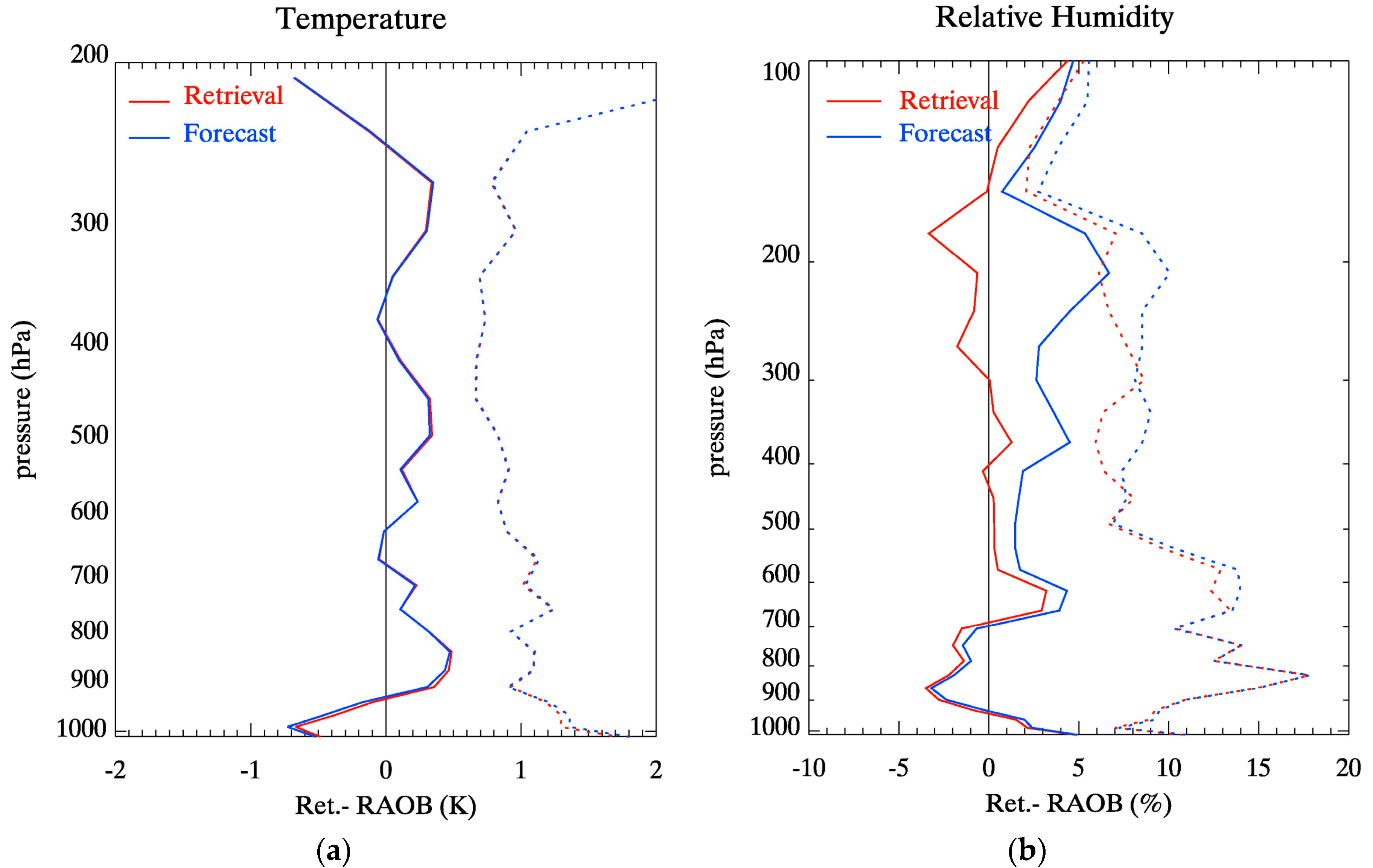
3.2.1. Retrieved Profiles
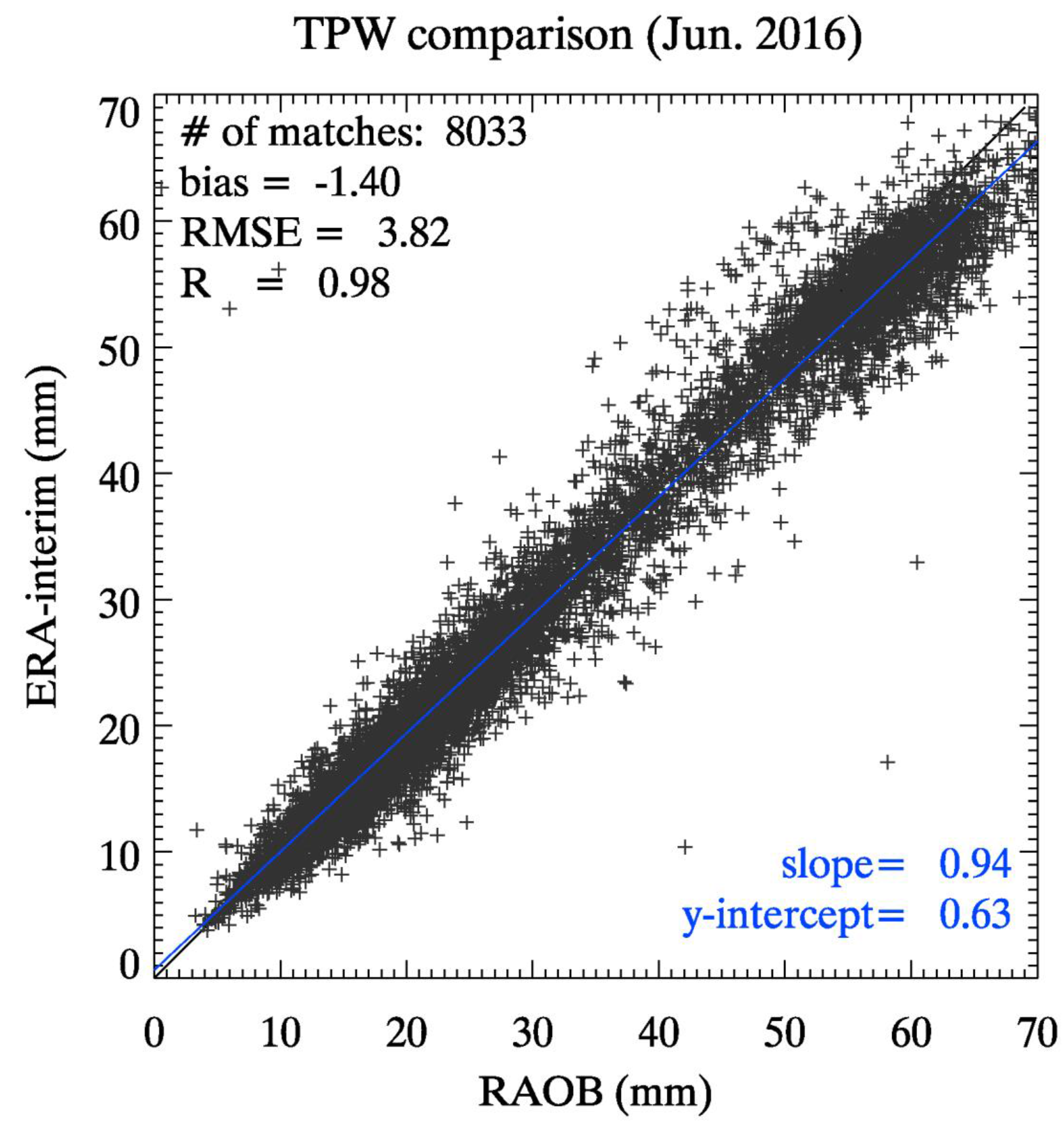
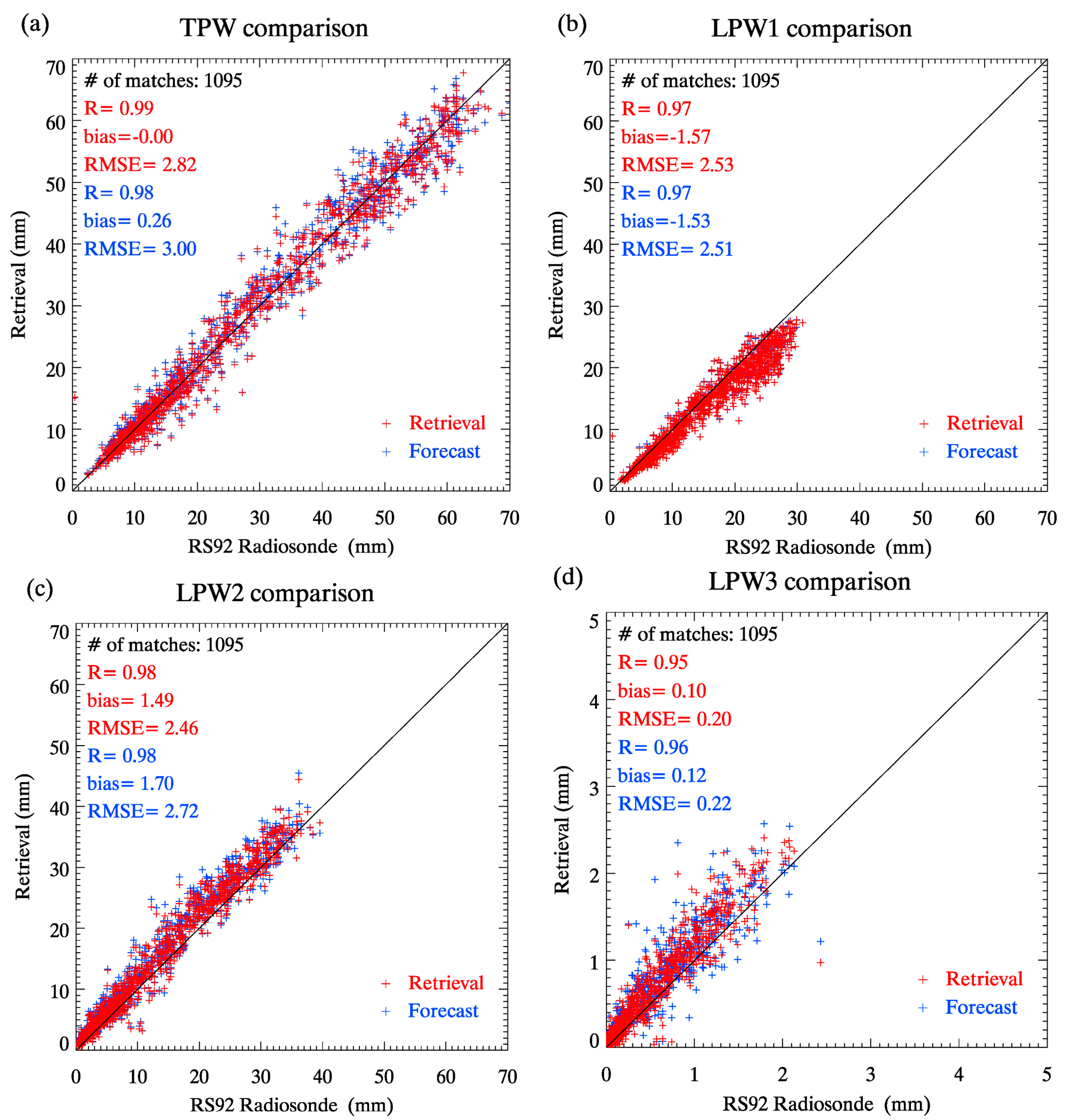
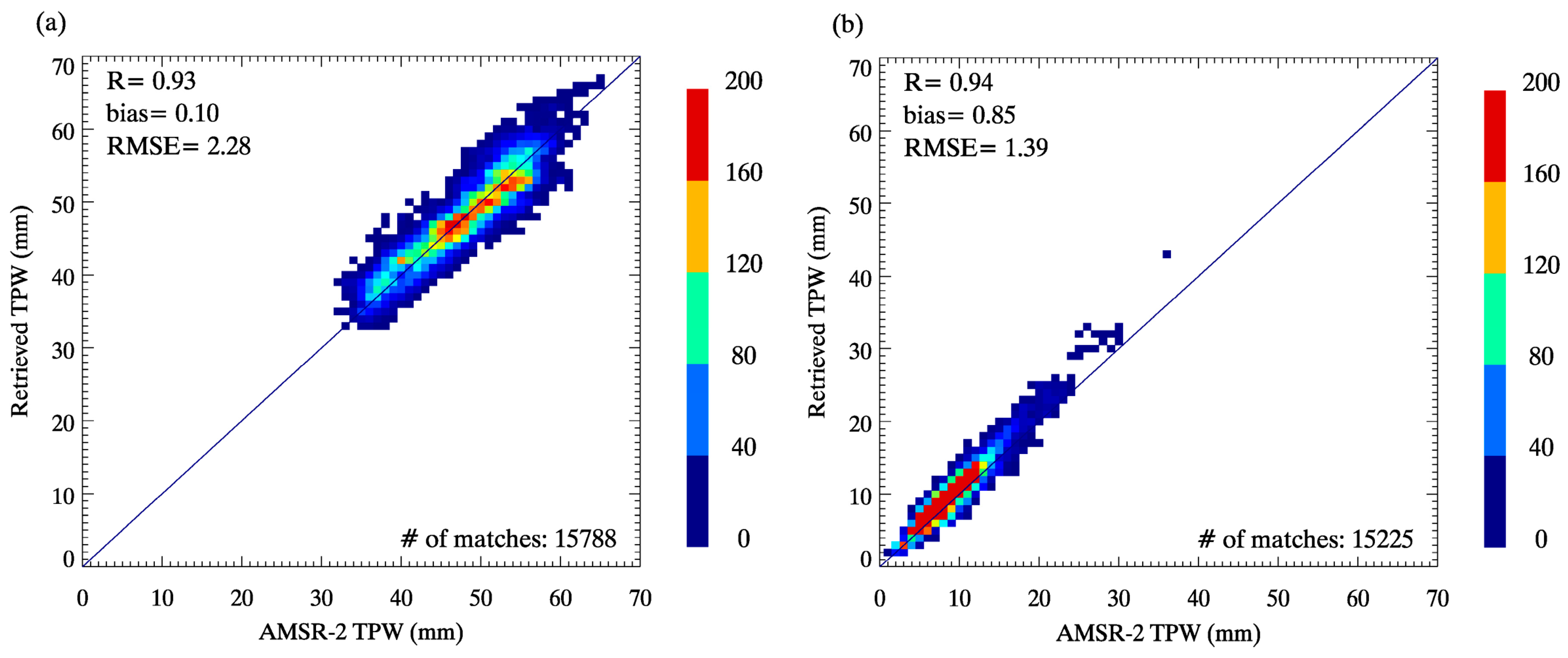
The accuracy of retrieved profiles on land was evaluated using radiosonde RS92 data from the stations located in Japan and Australia. For the comparison, the radiosonde profiles with more than ten point-measurements are selected and then interpolated to the RTTOV 54 pressure levels. The retrieved profiles are spatially averaged within 14 km × 14 km grid box centered on each radiosonde station. Total one month data (interval 12 h) from August 2016 is used and the results are shown in Figure 12 in terms of mean bias (retrieval − RAOB) and RMSE.
Improvements in the temperature profiles with retrieval are almost undetectable with 0.1 K bias and 1.1 K RMSE averaged between 200 and 1000 hPa. Previous studies with SEVIRI and simulated ABI [4] or GOES-13 Sounder [6] using a physical retrieval algorithm also showed little improvement in the retrieved temperature profile over the forecast. This is simply because NWP temperature forecasts are already in good accuracy and thus the retrieval algorithms are hard to improve the temperature profile over the forecast with just one sounding channel, i.e., the CO2 absorption channel (13.3 μm) of AHI or ABI. Meanwhile, both bias and RMSE profiles of relative humidity improve upon the forecasts throughout the atmospheric layers up to approximately 6% for bias and 4% for RMSE. The layer mean bias and RMSE between 100 and 1000 hPa is −0.0% and 9.0% for the retrieval and 1.9% and 9.8% for the forecast, respectively. Previous studies showed improvements in the retrieved relative humidity profile RMSE over the ECMWF forecast [4] or the NCEP GFS forecast [6] between 300 and 700 hPa in particular, while in this study the largest improvement over the forecast is seen in the upper atmosphere (above 300 hPa) than in the mid-atmosphere and this may require further investigation.

3.2.2. Derived TPW

TPW, together with atmospheric stability indices such as Lifted index or CAPE, is a good indicator of severe weather in the pre-convective atmospheric condition. Currently, geostationary satellite TPW products are available from the GOES sounders, the ABI on board the GOES-16 and from the SEVIRI on board the Meteosat 8, 9 and 10. Although microwave sensors provide accurate water vapor information in the lower troposphere, TPW from geostationary satellites can be efficiently used to trace the upper-level boundaries of water vapor and the location of tropopause folds or jets [35]. Particularly, retrieved precipitable water from multiple layers can be more useful since it provides information on the vertical distribution of water vapor and the differential moisture advection, which models do not forecast well. Also, it helps to diagnose the atmospheric motions at different levels [36]. For these reasons, the importance of LPW for operational forecasting applications has increased.
In order to see the contribution of AHI water vapor channels to the retrieval of water vapor concentration in multiple layers of the atmosphere, not only the TPW but also the retrieved LPW from three atmospheric layers are evaluated. For the evaluation of retrieval accuracy of these moisture-related products, one-month TPW and LPW (August 2016 with an interval of 12 h) measured from radiosonde stations using Vaisala RS92 type (DC3 and Auto) [31] are used. RAOB LPW values, which are not included in the provided radiosonde sounding parameters, are calculated from the given point-measured Q profiles.
The comparison result for TPW on land is shown in Figure 13a together with the results for the derived LPW1 (Figure 13b), LPW2 (Figure 13c) and LPW3 (Figure 13d). The statistics from approximately 1000 collocated matches within a 0.2-degree radius from the radiosonde stations show overall improvements in the retrievals (red) upon the UM forecasts (blue) in both total and layer integrated PW with a higher correlation (R) and a smaller mean bias and RMSE. Compared to other layers, the derived LPW between 850 and 400 hPa (Figure 13c) shows more improvement upon the forecast, in terms of the mean bias and RMSE, with higher correlation with the reference.
Figure 14 shows the comparison results of TPW over the ocean with AMSR2 measurements for the region of 30–40°N and 120–145°E, where the radiometer passes between 0320 and 0530 UTC in the afternoon (ascending) and 1600 and 1800 UTC at night (descending). The derived TPW are averaged within a 0.1-degree radius and within a 5 min time difference. Approximately 15,000 collocated data are compared for summer from August 2016 (Figure 14a) and for winter from Dec. 2016 (Figure 14b). As can be seen in the figures, retrieved TPW agrees well with the AMSR2 TPW for both summer and winter with smaller RMSE in winter than in moist summer. Compared to the previous study that evaluated the retrieved TPW from SEVIRI [4] and GOES-13 sounder [6] using the AMSR-Earth Observing System (AMSR-E) TPW over the ocean in August, the results in this study show a slightly smaller bias (0.1 mm) and RMSE (2.28 mm) and this result meets the requirements of GK-2A TPW products, which is 1 mm for mean bias and 3 mm for RMSE.

4. Discussion

The validation results presented in the study suggest that the moisture information from AHI improves the model forecasts in the mid- to upper-troposphere during the summer. With the improved profile accuracy, the estimated layered precipitable water over ocean for both summer and winter show an improvement over the first guess values. However, the retrieval accuracy of the moisture profile during the winter over the land has not been analyzed fully. According to a study on the retrieval accuracy of sounding products of the Infrared Atmospheric Sounding Interferometer over East Asia [37], the derived TPW shows higher RMSE over land under dry conditions, which corresponds to the winter condition in East Asia. This is because the transmittance in the water vapor channels increases when there is little amount of moisture in the atmosphere and then the outgoing radiance is influenced by the surface. Therefore, with focusing on these aspects, further evaluation is going to be performed for a longer period of time including data from each season.
It should also be noted that the retrieval accuracy depends on the convergence threshold applied to the algorithm. With a tighter convergence threshold, the retrieval accuracy increases but at the expense of retrieval rate, i.e., the rate of the number of clear-sky pixels over which retrievals are achieved to the total number of clear-sky pixels over which retrievals are attempted, as briefly mentioned in Section 3.1.2. With a comparatively relaxed convergence threshold (e.g., 0.7 K for the channel mean RMSE between the observation and retrieval), however, the retrieval rate increases but with reduced retrieval accuracy. The increased retrieval rate in the latter case provides smooth features in the retrieved field, which may include unfiltered clouds but also meaningful moisture information around cloud edges. Therefore, one might utilize the retrieved information within acceptable accuracy range according to the purpose.
Another important consideration regarding the retrieval accuracy in a retrieval process based on optimal estimation is, as emphasized in Section 2.2, the appropriate specification of errors related to the observation and the background. The study uses observation errors that are dynamically calculated according to the scene temperature but employs fixed background errors provided for 3 latitudinal bands. However, previous study [38] suggests that using a priori errors dynamically updated based on the atmospheric conditions can improve the accuracy of water vapor retrievals in the boundary layer in the physical retrieval results. Future work can consider dynamic background errors classified by TPW to improve the boundary layer retrieval.

5. Conclusions

In preparation of Korea’s next generation geostationary meteorological satellite, an iterative physical retrieval algorithm based on optimal estimation has been developed and applied to the real-time measurements from AHI. To constrain the solution, the 6–11 h forecast fields from the KMA global prediction model based on UM are introduced without regression. For the calculation of the forward model and Jacobians, RTTOV 11.2 is used and the required land surface emissivity data is generated using the monthly global emissivity database from CIMSS.
Like other new generation geostationary imagers, AHI has very limited number of infrared channels for sounding retrievals, providing information contents considerably smaller than that of a hyperspectral sounder. The evaluated DFS is far less than 1 for temperature but the study shows that much higher independent piece of information is provided from the three water vapor channels of AHI with mean DFS of about 2.3 (maximum of 3.6). The study also shows that the amount of information contents has a positive relationship with the number of iterations required in the iterative retrieval process both on land and ocean. The most sensitive altitude for the retrieval with respect to the change in true state was also analyzed via the vertical distribution of the rows of the averaging kernels, which have the peaks at around 960 hPa for temperature and 300 hPa for moisture for the case analyzed. The retrieval accuracy was evaluated by the comparison with a quality controlled radiosonde dataset measured from Vaisala RS92 type on land and with the AMSR2 products over the ocean. The comparison results show that the algorithm can retrieve temperature sounding information with accuracy comparable to the model forecasts while more useful moisture information is retrieved from AHI. The retrieved moisture profiles improve upon the forecast (or first-guess) profile with smaller bias (by 6%) and RMSE (by 4%) and the derived products, i.e., TPW and LPW, also show consistent improvements on the first guess throughout the troposphere. Considering the much finer spatial resolution of AMI or AHI that scan the full-disk within less than 10 min, the imager-driven information can be useful in the area of interest to fill the gap between polar-orbiting hyper-spectral sounders or ground-based observations.

Acknowledgments

This work was supported by “Development of AAP Algorithms” project, funded by ETRI, which is a subproject of “Development of Geostationary Meteorological Satellite Ground Segment (NMSC-2016-01)” program funded by NMSC (National Meteorological Satellite Center) of KMA (Korea Meteorological Administration).

Author Contributions

Myoung-Hwan Ahn conceived and designed the experiments; Su Jeong Lee performed the experiments, analyzed the data and wrote the paper; Sung-Rae Chung contributed to data acquisition and coordination of the project. All authors contributed to the edition of the manuscript.

Conflicts of Interest

The authors declare no conflict of interest.

References

  1. Ambrosetti, P. Statement of Guidance for Nowcasting and Very Short Range Forecasting (VSRF). World Meteorological Organization. Available online: http://www.wmo.int/pages/prog/www/OSY/SOG/SoG-Nowcasting-VSRF.pdf (accessed on 10 October 2017).
  2. Lee, J.; Lee, S.-W.; Han, S.-O.; Lee, S.-J.; Jang, D.-E. The Impact of Satellite Observations on the UM-4DVar Analysis and Prediction System at KMA. Atmos. Korean Meteorol. Soc. 2011, 21, 85–93. (In Korean) [Google Scholar]
  3. Schmit, T.J.; Li, J.; Gurka, J.J.; Goldberg, M.D.; Schrab, K.J.; Li, J.; Feltz, W.F. GOES-R Advanced Baseline Imager and the Continuation of Current Sounder Products. J. Appl. Meteorol. Climatol. 2008, 47, 2696–2711. [Google Scholar] [CrossRef]
  4. Jin, X.; Li, J.; Schmit, T.J.; Li, J.; Goldberg, M.D.; Gurka, J.J. Retrieving clear-sky atmospheric parameters from SEVIRI and ABI infrared radiances. J. Geophys. Res. 2008, 113. [Google Scholar] [CrossRef]
  5. Li, Z.; Li, J.; Menzel, W.P.; Schmit, T.J.; Nelson, J.P., III; Daniels, J.; Ackerman, S.A. GOES sounding improvement and applications to severe storm nowcasting. Geophys. Res. Lett. 2008, 35. [Google Scholar] [CrossRef]
  6. Lee, Y.-K.; Li, Z.; Li, J. Evaluation of the GOES-R ABI LAP Retrieval Algorithm Using the GOES-13 Sounder. J. Atmos. Ocean. Technol. 2014, 31, 3–19. [Google Scholar] [CrossRef]
  7. KMA. Status Report on the Current and Future Satellite Systems by KMA; Presented to CGMS-43 Plenary Session, Agenda Item [E.1]; University Corporation for Atmospheric Research (UCAR): Boulder, CO, USA, 2015. [Google Scholar]
  8. Rodgers, C.D. Retrieval of atmospheric temperature and composition from remote measurements of thermal radiation. Rev. Geophys. 1976, 14, 609–624. [Google Scholar] [CrossRef]
  9. Ma, X.L.; Schmit, T.J.; Smith, W.L. A nonlinear physical retrieval algorithm—Its application to the GOES-8/9 sounder. J. Appl. Meteorol. 1999, 38, 501–513. [Google Scholar] [CrossRef]
  10. Rodgers, C.D. Inverse Methods for Atmospheric Sounding: Theory and Practice; Taylor, F.W., Ed.; World Scientific Publishing: Singapore, 2000; Volume 2, pp. 21–41, 81–99. ISBN 981-02-2740-X. [Google Scholar]
  11. Li, J.; Schmit, T.J.; Jin, X.; Martin, G. GOES-R Advanced Baseline Imager (ABI) Algorithm Theoretical Basis Document for Legacy Atmospheric Moisture Profile, Legacy Atmospheric Temperature Profile, Total Precipitable Water and Derived Atmospheric Stability Indices; U.S. Department of Commerce: Washington, DC, USA; National Oceanic and Atmospheric Administration: Silver Spring, MD, USA; National Environmental Satellite, Data and Information Service: Silver Spring, MD, USA, 2012.
  12. Eyre, J.R. Inversion of cloudy satellite sounding radiances by nonlinear optimal estimation. I: Theory and simulation for TOVS. Q. J. R. Meteorol. Soc. 1989, 115, 1001–1026. [Google Scholar] [CrossRef]
  13. Matricardi, M.; Chevallier, F.; Kelly, G.; Thepaut, J.-N. An improved general fast radiative transfer model for the assimilation of radiance observations. Q. J. R. Meteorol. Soc. 2004, 130, 153–173. [Google Scholar] [CrossRef]
  14. Renshaw, R. Bias Correction Procedures for ATOVS—A Brief Guide: Bias Correction of (A)TOVS Radiances. Available online: http://nwpsaf.eu/oldsite/deliverables/aapp/biasguide.htm (accessed on 22 September 2017).
  15. Zou, X.; Zhuge, X.; Weng, F. Characterization of Bias of Advanced Himawari Imager Infrared Observations from NWP Background Simulations Using CRTM and RTTOV. J. Atmos. Ocean. Technol. 2016, 33, 2553–2567. [Google Scholar] [CrossRef]
  16. Hewison, T.J.; Wu, X.; Yu, F.; Tahara, Y.; Hu, X.; Kim, D.; Koenig, M. GSICS Inter-Calibration of Infrared Channels of Geostationary Imagers Using Metop/IASI. IEEE Trans. Geosci. Remote Sens. 2013, 51, 1160–1170. [Google Scholar] [CrossRef]
  17. McPeters, R.D.; Labow, G.J. Climatology 2011: An MLS and sonde derived ozone climatology for satellite retrieval algorithms. J. Geophys. Res. 2012, 117. [Google Scholar] [CrossRef]
  18. Ha, S.; Ahn, M.-H.; Lee, S.J. Possibility of an improved total ozone information from the high performance geostationary imager data. Presented at Asia Oceania Geosciences Society, Singapore, 6–11 August 2017. [Google Scholar]
  19. Bannister, R.N. A review of forecast error covariance statistics in atmospheric variational data assimilation. I: Characteristics and measurements of forecast error covariances. Q. J. R. Meteorol. Soc. 2008, 134, 1951–1970. [Google Scholar] [CrossRef]
  20. Stewart, L.M.; Dance, S.L.; Nichols, N.K. Data assimilation with correlated observation errors: Experiments with a 1-D shallow water model. Tellus A Dyn. Meteorol. Oceanogr. 2013, 65. [Google Scholar] [CrossRef] [Green Version]
  21. Yao, Z.; Li, J.; Li, J.; Zhang, H. Surface emissivity impact on temperature and moisture soundings from hyperspectral infrared radiance measurements. J. Appl. Meteorol. Climatol. 2011, 50, 1225–1235. [Google Scholar] [CrossRef]
  22. Li, J.; Li, J.; Weisz, E.; Schmit, T.; Goldberg, M.; Zhou, D. The simultaneous retrieval of hyperspectral IR emissivity spectrum along with temperature and moisture profiles from AIRS. Int. Soc. Opt. Eng. 2007, 66840L. [Google Scholar] [CrossRef]
  23. Seemann, S.W.; Borbas, E.E.; LI, J.; Menzel, W.P.; Gumley, L.E. MODIS Atmospheric Profile Retrieval Algorithm Theoretical Basis Document; ATBD07 Version 6; Cooperative Institute for Meteorological Satellite Studies, University of Wisconsin-Madison: Madison, WI, USA, 25 October 2006. [Google Scholar]
  24. Maddy, E.S.; Barnet, C.D. Vertical Resolution Estimates in Version 5 of AIRS Operational Retrievals. IEEE Trans. Geosci. Remote Sens. 2008, 46, 2375–2384. [Google Scholar] [CrossRef]
  25. Kokhanovsky, A.A.; de Leeuw, G. Satellite Aerosol Remote Sensing over Land; Springer Science & Business Media: Berlin, Germany, 2009; pp. 228–235. ISBN 978-3-540-69397-0. [Google Scholar]
  26. Chung, E.-S.; Soden, B.J.; Sohn, B.J.; Schmetz, J. An assessment of the diurnal variation of upper tropospheric humidity in reanalysis data sets. J. Geophys. Res. Atmos. 2013, 118, 3425–3430. [Google Scholar] [CrossRef]
  27. Noh, Y.-C.; Sohn, B.-J.; Kim, Y.; Joo, S.; Bell, W. Evaluation of temperature and humidity profiles of Unified Model and ECMWF analyses using GRUAN radiosonde observations. Atmosphere 2016, 7, 94. [Google Scholar] [CrossRef]
  28. Moradi, I.; Arkin, P.; Ferraro, R.; Eriksson, P.; Fetzer, E. Diurnal variation of tropospheric relative humidity in tropical regions. Atmos. Chem. Phys. 2016, 16, 6913–6929. [Google Scholar] [CrossRef]
  29. Sun, B.; Reale, A.; Seidel, D.J.; Hunt, D.C. Comparing radiosonde and COSMIC atmospheric profile data to quantify differences among radiosonde types and the effects of imperfect collocation on comparison statistics. J. Geophys. Res. 2010, 115. [Google Scholar] [CrossRef]
  30. Soden, B.J.; Lanzante, J.R. An assessment of satellite and radiosonde climatologies of upper tropospheric water vapor. J. Clim. 1996, 9, 1235–1250. [Google Scholar] [CrossRef]
  31. Ingleby, B. An Assessment of Different Radiosonde Types 2015/2016; ECMWF Technical Memorandum No. 807; European Centre for Medium Range Weather Forecasts: Reading, UK, 2017. [Google Scholar]
  32. Ingleby, B. On the Accuracy of Different Radiosonde Types—WMO. TECO-2016 Madrid, 30 September 2016. Available online: www.wmo.int/pages/prog/www/IMOP/meetings/Upper-Air/ET-IOC-3/Doc3.1(1).pdf (accessed on 11 August 2017).
  33. JAXA. Status of A R2 Level-2 Products (Algorithm Ver. 2.00). 2015. Available online: suzaku.eorc.jaxa.jp/GCOM_W/materials/product/AMSR2_L2_2.pdf (accessed on 25 September 2017).
  34. Duncan, D.I.; Kummerow, C.D. A 1DVAR retrieval applied to GMI: Algorithm description, validation and sensitivities. J. Geophys. Res. Atmos. 2016, 121, 7415–7429. [Google Scholar] [CrossRef]
  35. EUMETSAT. Product Tutorial on Total Precipitable Water Content Products. 2014. Available online: http://www.eumetrain.org/data/3/359/print_3.htm#page_1.0.0 (accessed on 11 October 2017).
  36. Li, J.; Gerth, J.; Lee, Y.-K.; Li, Z.; Schmit, T.J.; Wang, P.; Bachmeier, S. High resolution all-sky water vapor products from new generation of geostationary satellites and their applications in weather forecasts. Presented at the 7th Asia-Oceania Meteorological Satellite Users’ Conference, Songdo City, Korea, 24–27 October 2016. [Google Scholar]
  37. Kwon, E.-H.; Sohn, B.J.; Smith, W.L.; Li, J. Validating IASI temperature and moisture sounding retrievals over East Asia using radiosonde observations. J. Atmos. Ocean. Technol. 2012, 29, 1250–1262. [Google Scholar] [CrossRef]
  38. Kown, E.-H.; Li, J.; Li, J.; Shon, B.J.; Weisz, E. Use of total precipitable water classification of a priori error and quality control in atmospheric temperature and water vapor sounding retrieval. Adv. Atmos. Sci. 2012, 29, 263–273. [Google Scholar] [CrossRef]
Figure 1. Algorithm flowchart for the retrieval of clear-sky atmospheric profiles.
Remotesensing 09 01294 g001
Figure 2. Mean TB bias and root mean square difference (RMSD) between AHI and (a) simulated ERA TB over the ocean for 1–10 June 2016; (b) simulated RAOB TB over the land for one-month data from June 2016 under clear sky conditions.
Remotesensing 09 01294 g002
Figure 3. Validation of retrieved moisture profile with radiosonde data (from August 2016) before (black) and after (red) the bias correction compared to the model forecast (blue).
Remotesensing 09 01294 g003
Figure 4. Sensitivity of KS a K T to the change in (a) temperature and (b) moisture error covariance matrix.
Remotesensing 09 01294 g004
Figure 5. Monthly climatological land surface emissivity data for AHI channels (a) 8.6, (b) 9.6, (c) 10.4, (d) 11.2, (e) 12.4 and (f) 13.3 μm.
Remotesensing 09 01294 g005
Figure 6. Vertical averaging kernels (rows of AK) for (a) Temperature and (b) Moisture for a specific scene (00 UTC 1 August 2016) at a specific place (33.996N, 124.977E) corresponding to pressure levels (in colors) with the area of the AK (dotted line, scaled by a factor of 0.1 for moisture).
Remotesensing 09 01294 g006
Figure 7. (a) Degrees of freedom for (a) total; (b) temperature; and (c) moisture signal on 1 August 2016, 00 UTC.
Remotesensing 09 01294 g007
Figure 8. (a) the distribution of total DFS in the western part of Australia and (b) the profiles of Q DFS corresponding to the locations A, B, C and D in (a).
Remotesensing 09 01294 g008
Figure 9. (a) the relationship between the convergence thresholds and the percentage of successful clear-sky retrievals (red line) and the number of iterations required for the retrieval (b) the relationship between the number of iterations and corresponding mean total DFS from 19 different scenes on 1~10 August 2016.
Remotesensing 09 01294 g009
Figure 10. Time series of the background departure over the ocean (a) and land (c) and the retrieval departures over the ocean (b) and land (d) under clear-sky conditions for August 2016 (00/12 UTC).
Remotesensing 09 01294 g010
Figure 11. Comparisons of TPW from two different reference data (Radiosonde vs. ERA-interim) for June 2016.
Remotesensing 09 01294 g011
Figure 12. The bias (solid) and RMSE (dotted) profiles for (a) temperature and (b) relative humidity between radiosonde and retrieval (red) and UM forecast as background (blue).
Remotesensing 09 01294 g012
Figure 13. Comparison result of the retrieved (a) TPW (b) LPW1 (c) LPW2 (d) LPW3 with RAOB (RS92) for one month, August 2016.
Remotesensing 09 01294 g013
Figure 14. Comparison results of retrieved TPW and AMSR-2 measurements over the region between 30–45N and 120–145E for (a) summer and (b) winter.
Remotesensing 09 01294 g014
Table 1. Comparison of central wavelength of next generation geostationary imagers.
ChannelAMI GK-2AAHI Himawari-8ABI GOES-R
VIS0.470.460.47
0.510.51
0.640.640.64
0.8560.860.865
NIR1.38 1.378
1.611.61.61
2.32.25
SWIR3.83.93.90
IR6.26.26.185
6.956.96.95
7.37.37.34
8.68.68.50
9.69.69.61
10.410.410.35
11.211.211.2
12.3612.412.3
13.313.313.3
Table 2. Algorithm specification.
Measurements (TB)AHI TBs from 9 infrared channels (6.2, 6.9, 7.3, 8.6 *, 9.6, 10.4, 11.2, 12.4, 13.3)
First-Guess ( x a )T and Q: 6 to 11 h KMA UM forecast
O3: monthly climatology improved using OMI total ozone
Observation Error Covariance ( S ϵ )Error covariance for instrument noise (NEdT) and RTM error
Background Error Covariance ( S a )T and Q: B-matrix used in KMA OPS 1DVar
O3: B-matrix used in ECMWF 1DVar
LSEMonthly climatology generated from CIMSS global LSE database
RTMRTTOV v.11.2
8.6 *: used for retrievals over the ocean only.

