Article

Comparing and Merging Observation Data from Ka-Band Cloud Radar, C-Band Frequency-Modulated Continuous Wave Radar and Ceilometer Systems

1
State Key Laboratory of Severe Weather, Chinese Academy of Meteorological Sciences, Beijing 100086, China
2
Plateau Atmosphere and Environment Key Laboratory of Sichuan Province, School of Atmospheric Sciences, Chengdu University of Information Technology, Chengdu 610225, China
*
Author to whom correspondence should be addressed.
Remote Sens. 2017, 9(12), 1282; https://doi.org/10.3390/rs9121282
Submission received: 19 October 2017 / Revised: 4 December 2017 / Accepted: 7 December 2017 / Published: 10 December 2017
(This article belongs to the Section Atmospheric Remote Sensing)

Abstract

:
Field experiment in South China was undertaken to improve understanding of cloud and precipitation properties. Measurements of the vertical structures of non-precipitating and precipitating clouds were obtained using passive and active remote sensing equipment: a Ka-band cloud radar (CR) system, a C-band frequency modulated continuous wave vertical pointing radar (CVPR), a microwave radiometer and a laser ceilometer (CEIL). CR plays a key role in high-level cloud observation, whereas CVPR is important for observing low- and mid-level clouds and heavy precipitation. CEIL helps us diminish the effects of “clear-sky” in the planetary boundary layer. The experiment took place in Longmen, Guangdong Province, China from May to September of 2016. This study focuses on evaluating the ability of the two radars to deliver consistent observation data and develops an algorithm to merge the CR, CVPR and CEIL data. Cloud echo base, thickness, frequency of observed cloud types and reflectivity vertical distributions are analyzed in the radar data. Comparisons between the collocated data sets show that reflectivity biases between the CR three operating modes are less than 2 dB. The averaged difference between CR and CVPR reflectivity can be reduced with attenuation correction to 3.57 dB from the original 4.82 dB. No systemic biases were observed between velocity data collected in the three CR modes and CVPR. The corrected CR reflectivity and velocity data were then merged with the CVPR data and CEIL data to fill in the gaps during the heavy precipitation periods and reduce the effects of Bragg scattering and fog on cloud observations in the boundary layer. Meanwhile, the merging of velocity data with different Nyquist velocities and resolutions diminishes velocity folding to provide fine-grain information about cloud and precipitation dynamics. The three daily periods in which low-level clouds tended to occur were at sunrise, noon and sunset and large differences in the average reflectivity values were observed. Mid- and high-level clouds tended to occur at 1400 and 1800 BT. Few clouds were found between a height of 3 and 5 km.

Graphical Abstract

1. Introduction

Clouds have a distinct influence on weather and climate. Under certain dynamic, thermodynamic and microphysical conditions, clouds can begin precipitating. Understanding the variation of vertical reflectivity structures and cloud bases for various types of clouds under different dynamic conditions will improve the analysis of convective weather systems and the impacts of cloud dynamics on climate change [1]. Cloud observation also contributes to the aviation safety. No single wavelength ground-based radar has proven to be capable of detecting a wide variety of cloud and precipitation properties. Multi-wavelength vertical observing technology is a promising means to simultaneously obtain the vertical structures of cloud and precipitation systems. Accurate measurements of a wide range of cloud bases rely on integration data from both optical and active microwave remote sensors.
Various methods are available to observe cloud-base height, including visual estimation and sounding balloons [2], infrared radiometers [3] and cloud radar [4]. Visual estimation is the oldest and is still the main method used in the operational weather service. However, without uniform standards for visual estimation, this method requires considerable time and effort. The results are also subjective and discontinuous in both space and time [5]. Cloud base detection using sounding balloons depends on the observer, which introduces observation error. Infrared radiometers can receive cloud-base brightness temperatures, which can be used to retrieve the cloud-base height based on radiative transfer equations. Although this method can collect observations during day and night, the cloud-base brightness temperature measurements are affected by aerosols and water vapor content in the atmosphere. In addition, large biases are present in the measurements and the associated retrieval algorithm is complicated [6]. In recent years, a real-time, high-resolution data acquisition mode using laser ceilometers (CEIL) gradually has replaced older methods that are based on laser-pulse technology. Next-generation laser ceilometers are characterized by smart, portable and large dynamic range features for real-time observations [7]. Laser ceilometers perform well for when observing clouds that are visible from the ground but they are severely affected by haze and their capacity for multi-layer cloud observation is limited.
Cloud radar, especially millimeter-wave radar, makes use of the electromagnetic scattering characteristics of cloud particles. By analyzing radar echoes of clouds, we can understand their macro- and micro-structures. The advantage of cloud radar lies in its ability to penetrate clouds or precipitation layers to detect multi-layered structures. Using signal-processing technologies such as spectral analysis, pulse compression and non-coherent integration, systems with a variety of modes simultaneously detect clouds at different heights. In the Atmospheric Radiation Measurement (ARM) Program sponsored by the US Department of Energy, their Ka-band cloud radar using a traveling wave tube transmitter had only four operational modes prior to 1996 to conduct cyclic observations. Among the four modes, two were high-sensitivity modes with pulse compression technology used to detect high-level clouds, while the other two modes without pulse compression were used to detect low-level clouds and precipitation. At 5-km altitude, the minimum detectable echo intensity could be up to −49 dBZ [8]. Since 1997, several extra operational modes were added, including pulse repetition frequency and coherent and non-coherent integration, which reduced the minimum detectable echo intensity to −54 dBZ [9]. Later, Clothiaux et al. proposed a multi-mode data merging method and compared the cloud radar observation results with CEIL observations of cloud-base height. Based on this work, they developed an approach to identify the cloud-base height by combining cloud radar and ceilometer observations [4].
To observe a full spectrum of cloud populations, data from a Ka-band vertical pointing cloud radar, C-band and S-band scanning weather radar were merged to construct a cloud-precipitation radar dataset [10]. Li et al. compared observations from a Ka-band cloud radar and from a ceilometer in Beijing, China. They found that the difference in the cloud-base height measurements from the cloud radar and ceilometer was less than 300 m and that haze had significant impacts on the ceilometer observations [11]. The cloud radar acquired much more high-level cloud valid data than did the CEIL, with similar amounts of mid-level cloud occurrence in the data sets, whereas the CEIL acquired more low-level valid cloud data than did the cloud radar. However, this study excluded precipitating clouds from its analysis [11]. Huang et al. analyzed cloud-base height observations from laser ceilometers with different wavelengths and transmitting powers, two cloud infrared radiometers, a whole sky imager and a cloud radar [5]. Their results indicate that (i) observations from the three laser ceilometers were consistent; (ii) low-level cloud observations from the two cloud infrared radiometers were slightly inconsistent; (iii) large discrepancies occurred in the observations of the low-level cloud-base height by cloud radar and by laser ceilometers; and (iv) observations from the infrared radiometers and the cloud radar were consistent. The cloud radar performs better for observing convective clouds but cannot provide effective observations of thin clouds [12,13].
Pulse Doppler radar uses narrow pulse transmissions to improve detection resolution. However, its wide receiver bandwidth reduces the radar sensitivity. The pulse compression technique can raise the signal to noise ratio and directly improve the detection capability, however, it increases the minimum detectable range. Thus, Pulse Doppler radar presents challenges in obtaining a wide range of signal resolutions without sacrificing minimum detectable range. Frequency-modulated continuous wave (FMCW) radar could observe a wide range of measurements by modulating the transmission signal frequency. FMCW radar is characterized by highly accuracy of range and velocity measurements, small minimum detectable range and low peak transmitted power. Since the late 1960s when FMCW techniques were first applied to cloud and precipitation remote sensing, an S-band FMCW radar developed in the US Naval Electronics Laboratory has been used to study the planetary boundary layer (PBL) structures [14], including temperature changes caused by turbulence and the impacts of vertical velocity on PBL stability [15]. Since the 21st century, Fast Fourier Transform (FFT) has been applied for radar data processing to obtain power spectra. In 2002, sponsored by the US DOE, an S-band FMCW radar with 1-m spatial and 1-s temporal resolutions was developed in the University of Massachusetts [16], which later was used to study convective triggering in the PBL, the water vapor mixing ratio, turbulent mixing and other parameters in PBL [17]. A recently developed portable K-band FMCW micro-rain radar (MRR) operates at the frequency of 24.1 GHz [18] and is mainly used to study microphysical parameters of weak precipitation [19].
A Ka-band solid-state transmitter cloud radar (CR) and a C-band FMCW radar (CVPR) have been developed in the Chinese Academy of Meteorological Sciences (CAMS). The two radars were installed at the Tibetan Plateau Meteorological Science experiment in 2014 and 2015, together with CEILs and microwave radiometers. Liu et al. analyzed the CR data about vertical structures of clouds and precipitation over the Tibetan Plateau and compared observations from the three CR operation modes. Subsequently, an algorithm to merge data collected under the three modes was proposed [20,21]. CVPR was tested in precipitation observations in Anhui, China and results reveal that the differences in radar reflectivity between the CVPR and the operational new-generation weather radar were less than 1 dB [22]. However, comparisons between the CR and CVPR observations have not yet been studied and a merged radar database from both of radars has not yet been constructed.
CR and CVPR were used to observe clouds and precipitation over the southern part of Guangdong Province from early May to Mid-June of 2013–2015 field campaign of the Southern China Monsoon Rainfall Experiment to improve the quantitative precipitation forecasts (QPFs) but unfortunately, few heavy rainfall events were observed [23]. To make up for this data set, we observed the vertical structures of clouds and precipitation in rainstorms over the northern part of Guangdong Province by both CR and CVPR at Longmen station during the summer of 2016.
In drought areas, the precipitation attenuation and insects have negligible effects on cloud measurements by CR. However, Guangdong Province has a sub-tropic climate. It is warm, moist and rainy during the summer. Since CR radar wave attenuates quickly in precipitation compared to longer wavelength radars, precipitation and insects may indeed present a real challenge for CR observations at this location during the summer. In addition, the CRs with solid-state transmitters appear to have serious limitations in detecting clouds within 2 km of the boundary layer [21].
The main purposes of this paper are to use CVPR and CEIL data to supplement the above-mentioned deficiency of CR and improve its cloud detection capability. Thus, the objectives of this study are to (i) investigate the cloud and precipitation detecting capabilities of the above–mentioned two radars and CEIL during 1-month continuous observations; (ii) reveal any bias related to the observations; (iii) develop an algorithm to merge the observations from CR, CVPR and CEIL to improve detections of heavy precipitation and shallow clouds.
The paper is organized as follows. Section 2 describes the main technical parameters of the two radar systems and instruments used in this study and Data merging algorithm for CR, CVPR and CEIL. Section 3 compares results from the different radars and CEIL and introduces a statistical analysis of hydrometeor observation from CR and CVPR. Section 4 discusses the effects of Mie scattering on reflectivity and velocity by CR and CVPR. A summary and conclusion are given in the final section.

2. Materials and Methods

2.1. Data and Instrument Description

Intensive cloud and precipitation observations were performed at Longmen Meteorological Bureau, Guangdong Province (114.25°E, 23.783°N, 86 m) from 1 June to 31 July 2016, with continuous observations occurring taken over the month of July. The instruments for vertical cloud structure observations included a CR, CVPR, CEIL, a micro-rain radar (MRR), a microwave radiometer and a disdrometer.

2.1.1. Cloud Radar (CR)

The CR with a solid-state transmitter adopts Doppler radar and polarization radar technology. It works in a vertically pointing mode to obtain vertical profiles of reflectivity Z, radial velocity Vr, velocity spectrum width Sw and the depolarization factor LDR in cloud and light precipitation. It also records the Doppler spectral density data Sz. Table 1 lists the main technical specifications. The main purpose in using the solid-state transmitter is to realize continuous measurements, since long-term cloud characteristics are especially important for cloud and precipitation physics. In order to improve the detection capability for clouds and precipitation, three operating modes are employed: the boundary mode (CR1), the cirrus mode (CR2) and the precipitation mode (CR3). Different radar pulse widths and coherent and incoherent integration techniques are used to meet the requirements for low-level and weak cloud detections. Major operational parameters are listed Table 2, including the number of range gates (Num_gate), the range sample volume spacing (R_space), the maximum range (R_max), the minimum range (R_min), the pulse width (τ), the pulse repetition frequency (PRF), the number of coherent integration (Ncoh), the number of incoherent integration (Nncoh), the number of fast Fourier transform (FFT) points (NFFT) and the radial velocity resolution (ΔV). More importantly, the coherent integration is applied before the FFT and the FFTs then are incoherently averaged. CR1 is suitable for cloud observation near the surface with high resolution of radial velocity. CR2 is important for weak cloud observations and radiation studies with its high sensitivity and large minimum range but CR2 cannot observe clouds and precipitation below the heights of 2.1 km. By comparison, CR3 with its low sensitivity in reflectivity and large Nyquist velocity is important for precipitation observations. In principle, it is desirable to use all three modes in concert to observe weak clouds and precipitation from near the ground to 15-km height. In the cloud radar observations, each mode operates in succession. Once the radial measurement is finished in one mode, the radar immediately switches to another mode. So, typically, the observations collected by the three different modes are recorded separately. One cycle of the three operational modes takes about 9 s and 400 complete cycles can be obtained within a 1-h period.

2.1.2. C-Band FMCW Radar (CVPR)

CVPR was the first FMCW radar system used in China for cloud and precipitation observations. The major technical parameters are listed in Table 3. It utilizes FMCW operational mode and Doppler radar technique to measure the reflectivity, radial velocity and velocity spectrum width of cloud and precipitation structures at various levels with vertical resolution of 30 m and temporal resolution of 2–3 s. The main difference between CR and CVPR is in radar wavelength, operational mode (pulse or FMCW) and beam width. CVPR is used to fill in gaps during periods of heavy precipitation and for low-level cloud observations. The CVPR we used was tested and calibrated by the manufacturer. When the CVPR data and data from China’s operational S-band Doppler radar (CINRAD/SA) are compared, the resulting reflectivity bias is less than 1dB [22].
Using valid radar measurements (greater than the specified SNR threshold of −12 dB for CR and −24 dB for CVPR, respectively), we obtained the minimum detectable reflectivities and the variations with height for CR’s modes and CVPR, based on statistical values at different heights (Figure 1). The CR’s minimum detectable reflectivities are closely related to pulse compressions and the number of coherent integrations. Compared with the CR3 mode, four times of coherent integration number is performed for the CR1 mode and the minimum detectable reflectivity is reduced by 6 dB. Similarly, two times of coherent integration is performed for the CR2 mode and the pulse compression ratio is 60, so the minimum detectable reflectivity can be theoretically reduced by 20.8 dB.
The CVPR minimum detectable reflectivity is 7 dB smaller than that of CR1, so we use the CVPR to supplement the CR data’s deficiencies in low altitudes and diminish the effects of precipitation attenuation on cloud detection in upper levels. The CR2 minimum detectable reflectivity is 8 dB smaller than that of CVPR, so we use the CR2 to supplement the CVPR data’s deficiencies in weak cloud in middle and high altitudes. In addition, the comparison between CR and CEIL data is useful to analyze the effect of Bragg scattering (i.e., clear-air return) on CVPR observation. The analysis above considers only the minimum detectable signal for each radar and assumes negligible path-integrated attenuation.

2.1.3. The Laser Ceilometers (CEIL)

The CL51 ceilometer, made by the Vaisala Company, employs a pulsed diode laser Light Detection and Ranging (LIDAR) technology, which can emit short powerful laser pulses in a vertical or near-vertical direction. The light reflected from haze, fogs, clouds, precipitation, or other obscurations is received and processed by the laser ceilometer to produce backscatter profiles. Meanwhile, the cloud base height can also be detected. A maximum of three cloud layers can be detected with vertical visibility. Table 4 lists the major parameters. The CEIL helps us to remove non-cloud-precipitation echoes from radar data in PBL.

2.1.4. The Microwave Radiometer

The MP-3000A microwave radiometer (MWR) we used has as many as 35 frequency channels to provide high temporal resolution atmospheric profiles for temperature, relative humidity (RH) and liquid water content up to 10 km altitude. The instrument includes sensors to measure surface pressure, surface temperature and surface relative humidity. These MWR data are used to examine the radar reflectivity in the PBL. The MWR data are available only for the month June in our dataset.

2.1.5. The Disdrometer

The HSC-OTT disdrometer is mainly based laser measurements and can measure the raindrop size distribution (DSD) and falling velocity. Precipitation particles were divided into 32 grades according to the equivalent volume diameter and falling velocity. The ranges of the diameter and velocity measurements were 0.062~24.5 mm and 0.05~20.8 m·s−1 with temporal resolution of 60 s. In addition, the data set included weather codes, precipitation rate and amount and reflectivity. Details are listed in Table 5. Wu and Liu compared the rain drop size distribution data in South China and Tibetan Plateau from the disdrometer and found precipitation over South China had more small drops in Wu and Liu [24].

2.2. Methods

2.2.1. Simulation of Differences in Reflectivity and Velocity by CR and CVPR

In order to analyze the differences in reflectivity and velocity observed by the CR and CVPR, the backscattering cross sections of oblate spheroid raindrops and solid ice spheres were computed for Ka and C band radar for Mie scattering by using the extended boundary condition method [25]. The size, shapes and structures of ice particles (crystal, snow, graupel and hail) are complicated. When falling, these particles rotate. For simplicity, the scattering was only calculated for the solid ice spheres, other complicated situations were no considered in this paper. The backscattering cross sections are normalized by the constant C given in Equation (1)
C = λ 4 π 5 | m 2 1 m 2 + 1 | 2
where, λ is the wavelength and m is the complex refractive index. The raindrop size distribution data observed by the disdrometer at the observation site were used to evaluate the reflectivity difference introduced by the different wavelengths used in CR and CVPR.

2.2.2. Comparison of Observations from Radars and CEIL

To compare the reflectivity measurements from the above-mentioned two radars and the CEIL-derived cloud-base height, attenuation correction was applied to the CR data according to Wang’s algorithm [26]. In the attenuation correction process, the attenuation coefficients for non-precipitating liquid clouds, precipitating liquid clouds and snow used in this paper are expressed as:
K = 1.1079 Z 0.49   for non-precipitating liquid cloud
K = 0.0003 Z 0.44   for snow
K = 0.0001 Z 0.93   for precipitating cloud
where, K is the attenuation coefficient (dB·km−1) and Z is reflectivity (mm6 ·m−3).
The time-height series of the CVPR and CEIL measurements were reconstructed to correlate with the CR observations. Since the temporal resolution is 9 s for the CR observations, 2–3 s for CVPR and 2–3 s for CEIL, the CVPR and CEIL data were sub-sampled to a 30-m and 9-s temporal and vertical resolution grids, respectively, to match the CR data’s temporal resolution.

2.2.3. Data Merging Algorithm for CR, CVPR and CEIL

The CR1 mode has high sensitivity and fine velocity resolution for observing boundary-layer clouds, which are often composed of small droplets. The CR2 has the highest available sensitivity and a long minimum range, which is suitable for observing weakly reflective and high-altitude clouds. The CR3 mode has large Nyquist velocity, large maximum reflectivity and a short minimum range, which is suitable for observing light precipitation. The CR suffers from attenuation in rainfall, while the CVPR reflectivity and velocity suffer slight attenuation and Mie scattering effects. CVPR has larger Nyquist velocity and higher sensitivity than CR1 and CR3 at altitudes below 2.1 km but it is affected by Bragg scattering in the boundary layer.
In order to produce a seamlessly merged data set for radar reflectivity and velocity, improving on CR’s detection ability for precipitation and low-level clouds in moist and rainy areas, observations from the two different types of radars and CEIL can be merged. This will also reduce attenuation and Mie scattering effects on reflectivity and velocity, helping to distinguish the cloud base with CEIL data during precipitation. Several key issues in merging the observations need to be considered: (i) The reliability of observations: In data merging, we should minimize the effects of pulse coding while keeping data with relatively large signal-to-noise ratios (SNR), both radars can provide high-quality observations of reflectivity and radial velocity when SNR exceeds a specified threshold of 10 dB greater than the minimum detectable SNR ( the specified SNR threshold of −12 dB for CR and −24 dB for CVPR, respectively) [4], when SNR is less than the threshold, obvious bias will occur in radar observations. Priorities are given to these reflectivity data with SNR larger than the specified thresholds in data merging. (ii) The signal attenuation of CR: due to the strong attenuation of CR’s signal in regions with heavy precipitating, the reflectivity of precipitation is often severely underestimated and sometimes the associated signals are even totally missed. (iii) Over-saturation: The dynamic ranges of the CR and CVPR are about 70 and 80 dB, respectively. Once the reflectivity is beyond this range, biases will occur in the measurements. (iv) Mie scattering effects on CR reflectivity and velocity: reflectivity differences between C-band and Ka-band wavelengths are obvious for relatively large hydrometeor particles. (v) Radial velocity aliasing: When large particles or strong vertical motions occur, coherent integration will lead to radial velocity aliasing in data from the CR1 and CR2 modes. The Nyquist velocities (Vmax) for the CR3 mode and CVPR are 18.67 and 22 m·s−1, respectively. Compared with the CR3 mode, four times of coherent integration number is performed for the CR1 mode and two times of coherent integration is performed for the CR2 mode. The Nyquist velocities (Vmax) for the CR1 mode and CR2 mode are reduced 4.67 and 9.34 m·s−1, respectively (Table 2). Velocity aliasing seldom occurs for CR3 mode and CVPR. (vi) radial velocity resolution: The resolution is the highest for the CR1 mode (0.018 m·s−1) and lowest for CVPR (0.0895 m·s−1). High-resolution data should be used when other parameters meet the requirements. For clouds and weak precipitation, the velocity resolutions are important to analyze air velocity and retrieve water content. (vii) Radar clutter and non-meteorological signals: special attention should be paid to the analyzing the reliability of CVPR echoes in the PBL based on the CEIL observations.
Therefore, merging data from different sources should follow these principles: (i) Correct the reflectivity biases for CR1 and CR2 in comparison with CR3, which are introduced by different numbers of incoherent and coherent integrations; correct the attenuation for CR data according to the attenuation coefficient and adjust reflectivity differences between corrected CR and CVPR, which are produced by systematic bias between CR and VPR and the Mie scattering effects in CR data. (ii) When radial velocity aliasing occurs, use data from the CR3 mode and CVPR, which provides the largest Nyquist radial velocity. (iii) when reflectivity saturation occurs, use data from low-sensitivity modes such as CR3 and CVPR. (iv) when SNR is large enough for other modes, avoid using data from the CR2 mode. (v) more valid data are available, if the reflectivity difference is less than defined threshold values, for example, 2 dB, use the data with fine velocity resolution. In other case, use an observation with larger reflectivity to reduce the CR’s signal attenuation effects on merged data. (vi) Because the beam widths of CVPR and CR are 2.6° and 0.35°, respectively, in a radar bin, reflectivity and radial velocity should be drawn from the same radar to produce contiguous regions in the grid and ensure both data points are from the same target scattering volume. In addition, in the merging algorithm, a pair of reflectivity and velocity values are treated as an entity and used to determine the source of the merged data. In some cases, only reflectivity or velocity would not decide which value is best. (vii) to aid in the identification of hydrometeor contributions to the final merged data, we generate a best estimate cloud-base height from the CEIL and radars. We assume that the CEIL is able to accurately detect the cloud base in non-precipitating clouds. However, this assumption becomes increasingly poor as the number of precipitation particles near and below cloud base increases [4]. When precipitation particles appear, the reflectivity increase. For these reasons, non-precipitating clouds with reflectivity weaker than a threshold below the CEIL-derived cloud-base heights are regarded as clutters (non-cloud-precipitation echoes), which are caused by insects, dusts, Bragg scatter and fog. The threshold is determined by analyzing the reflectivity below the CEIL (Figure 2). (viii) the CEIL-derived cloud-base within precipitation is then distinguished.
Based on the above discussion, merging the reflectivity and radial velocity from the three CR modes and CVPR requires the following steps:
(i)
Delete all noise data below a given SNR threshold of −12 dB for CR and −24 dB for CVPR and invalidate the data below the corresponding minimum detectable range.
(ii)
Sub-sample the CVPR observed reflectivity and velocity and the CEIL-derived cloud-base heights to fit the CR time-height grid. Temporal resolution of 9 s and a vertical resolution of 30 m are chosen for the present study. After obtaining the grid-point data in the time-height cross sections, the following procedures need to be performed:
(iii)
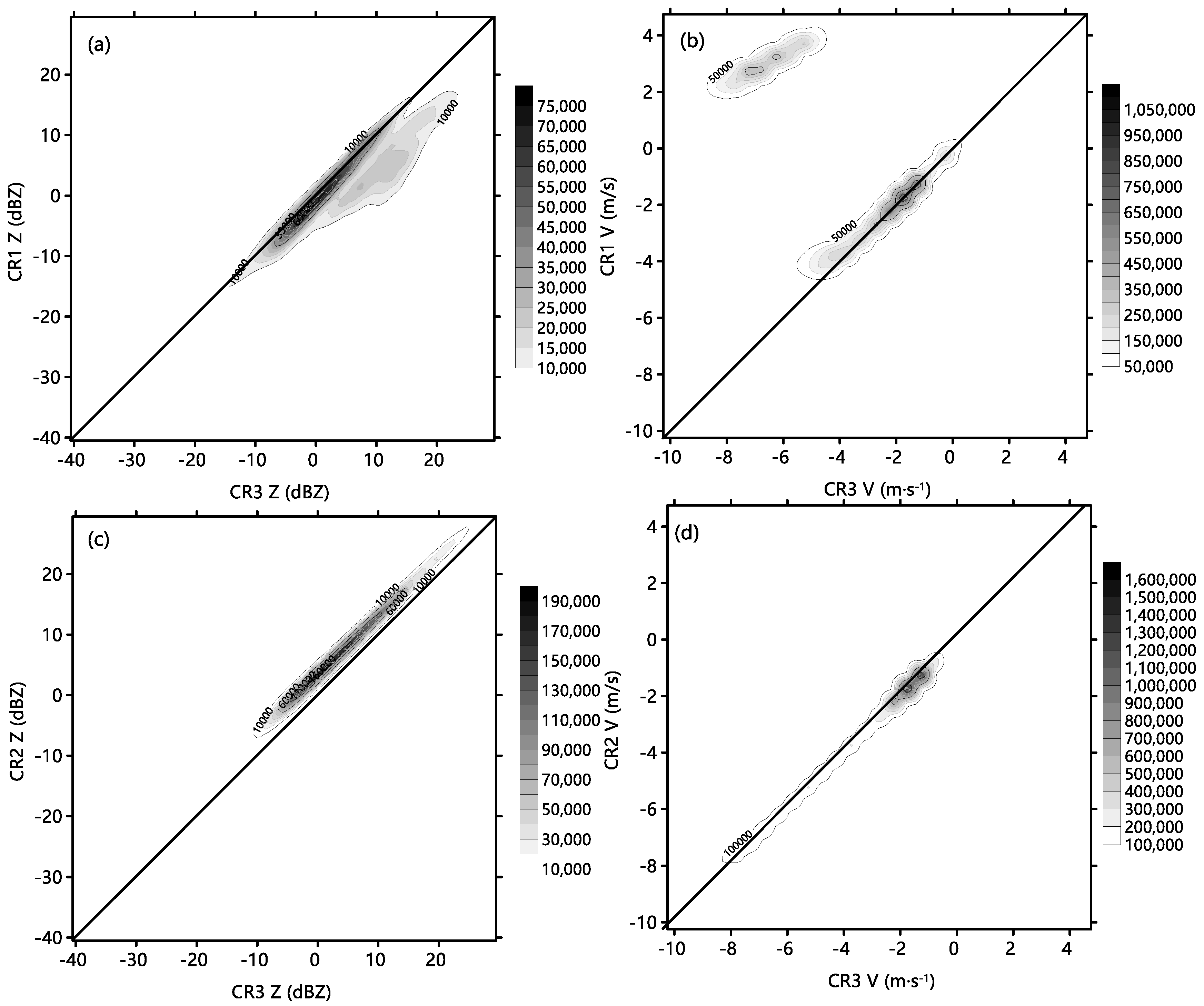
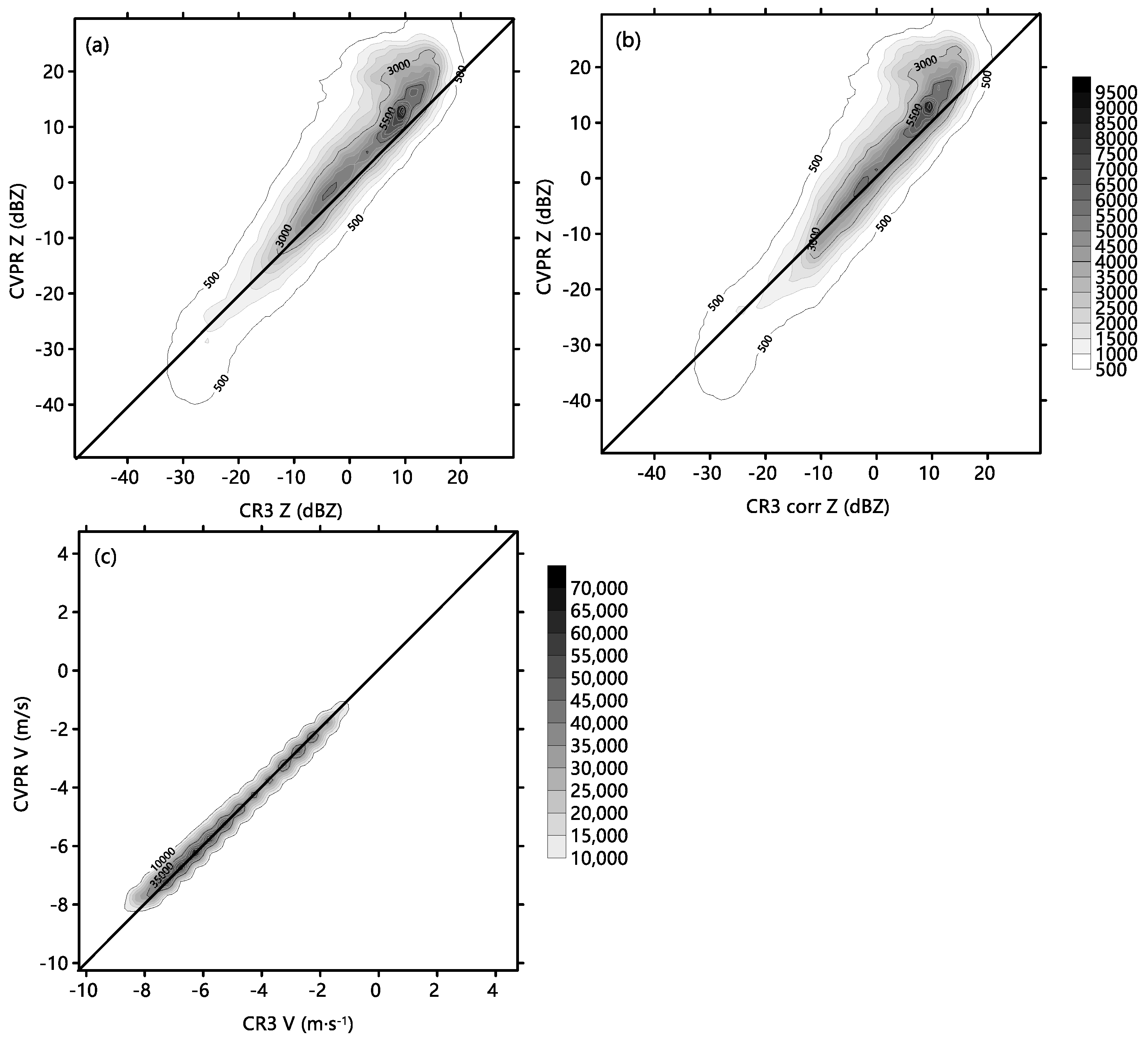
Correct for difference of reflectivity between CR1, CR2 and CR3 modes, which are produced by different numbers of incoherent and coherent integrations. Using the following reflectivity difference analysis for CR modes, the reflectivity values obtained by the CR1 and CR2 mode are corrected (minus 2 dB from the CR2 observed reflectivity, plus 2 dB from the CR1 observed reflectivity). Then, attenuation correction of CR reflectivity is conducted. Corrected CR reflectivity is adjusted to reduce the difference between CR and CVPR due to Mie scattering, systemic bias between CR and CVPR by Equation (5).
Z = 4.58 + 1.12 Z K A + 0.008 Z K A 2
where ZKA is CR observed reflectivity after corrections for attenuation and systemic bias. In this study, Equation (5) was fitted by using corrected CR reflectivity and CVPR data taken from 1 to 31 July 2016.
(iv)
Vmax, SNR and over saturation of reflectivity are utilized as criteria to determine the valid data for use in the merged data set. The minimum detectable reflectivity plus the corresponding dynamic range of reflectivity can be regarded as the maximum detectable reflectivity. If the reflectivity obtained by the CR3 mode or CVPR is larger than the maximum reflectivity from the CR1 mode or CR2 mode, or if the CR3 or CVPR velocity exceeds the CR1 or CR2 Nyquist velocity, data from the CR1 mode or CR2 is marked as “invalid”.
(v)
CR1, CR2 and CR3 data points are merged into one “best” value using the Liu’s algorithm [21]. If there are two valid data from CR and CVPR in a grid, the data with larger reflectivity are chosen when the reflectivity difference is larger than 2 dB to reduce the attenuation effects on merged data, otherwise, if the reflectivity difference is not obvious, the data with finer velocity resolution are chosen to ensure velocity quality.
(vi)
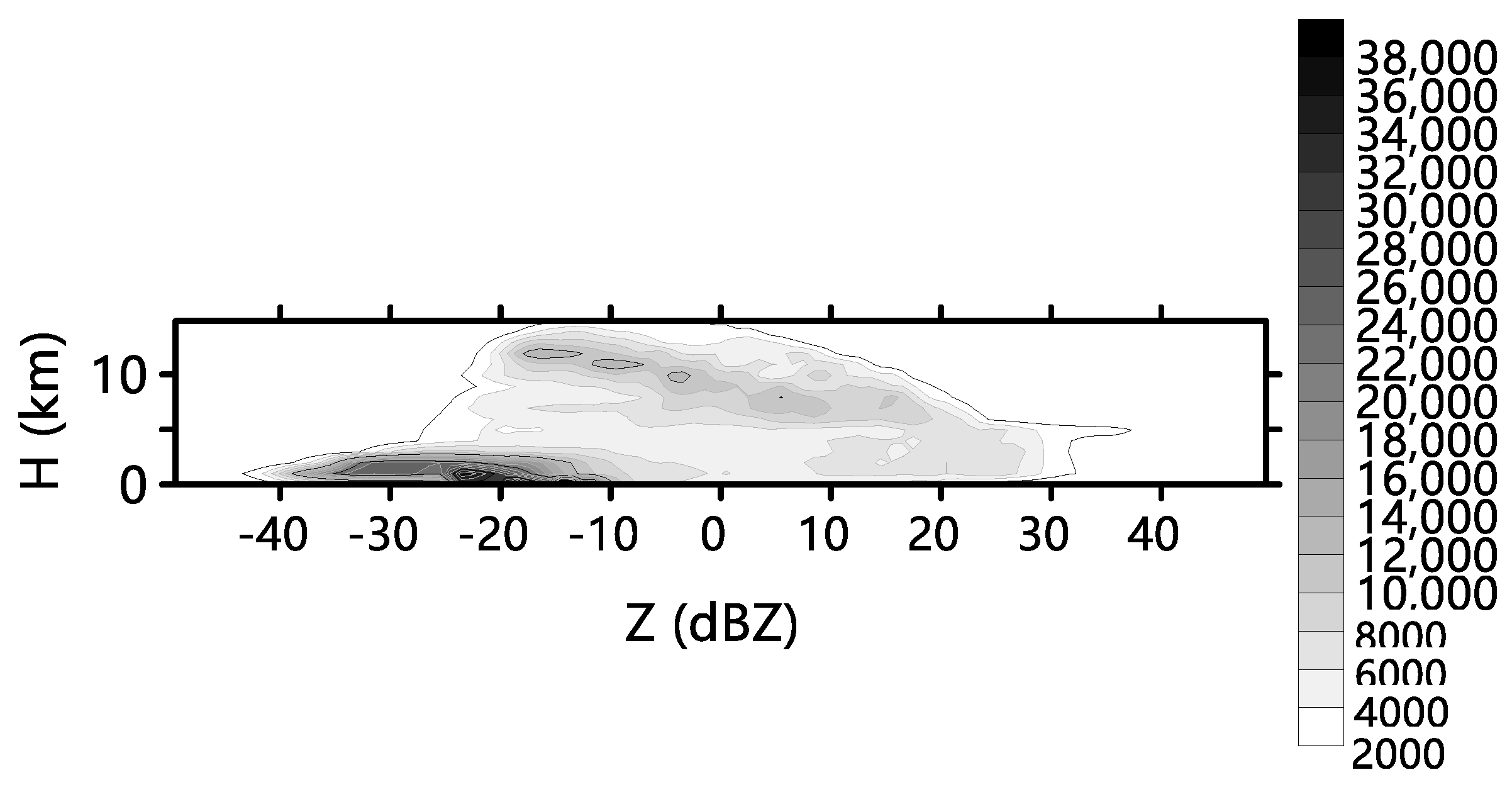
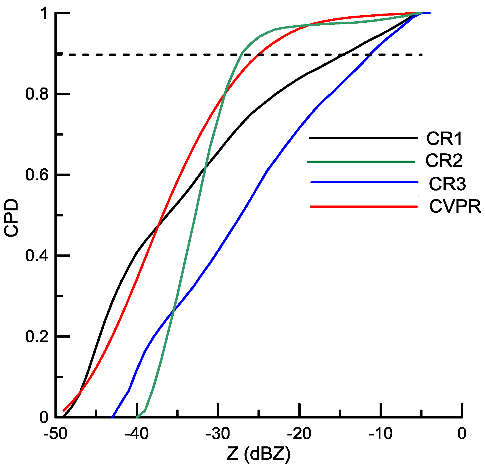
The radar data was flagged for clutters (no clouds and precipitation echo, such as insects, dust, Bragg scatter and fog echoes below the CEIL-derived cloud-base heights) by using the CEIL data following closely the method proposed by Clothiaux assuming that the CEIL-derived cloud-base heights are accurate [4]. We also distinguish precipitation from clutter in each radar profile that appears below the CEIL-derived cloud base height using “clear-sky” radar profiles. In this paper, clutter means non-cloud and precipitation echo, such as ground clutter, insect, dust, Bragg scatter and fogs echoes below the CEIL-derived cloud-base heights. Reflectivity during the period with the absence of significant radar returns above the CEIL-derived cloud-base heights were detected as “clear-sky” radar profiles. The “clear-sky” radar data taken during 1–31 July 2016 were statistically analyzed to obtain the cumulative probability distribution of “clear sky” reflectivity by CR1, CR2, CR3 and CVPR as shown in Figure 2. CR1, CR2, CR3 and CVPR, respectively, detected 31,078, 6552, 16,684 and 269,885 “clear-sky” echo points. If 90% of “clear-sky” echo points are flagged as clutter, the reflectivity thresholds for identifying clutter in CR1, CR2, CR3 and CVPR data below the CEIL-derived cloud-base heights were set to −14, −27, −11.0 and −24 dBZ. If reflectivity below the CEIL-derived cloud base was lower than the threshold, the data was flagged as clutter. Finally, the source of each data was recorded (from either CR or CVPR).
After merging the data from CR, CVPR and CEIL, the merged reflectivity and velocity data sets were finalized and clutter data in the merged data were flagged. The CEIL-derived cloud-base heights within the precipitation were also flagged.

3. Results

3.1. Comparison of Observations from Radars and CEIL

Figure 3 presents an example of a time-height cross sections of reflectivity from the CR modes and CVPR on 4 June 2016, along with CEIL-derived cloud-base heights. Several issues are apparent in the CR and CVPR time-height series reconstructed data. For the sake of convenience, clouds were categorized into low-level clouds with cloud-base height below 2.5 km, mid-level clouds with cloud-base height between 2.5 and 4.5 km and high-level clouds with cloud-base height above 4.5 km. Low-level clouds include clouds and precipitation detected by CR and CVPR and high-level clouds include those beyond the detectable range of the CEIL. During the observation period, nine precipitating convective cloud systems passed by the observing site, with bright bands at 5.8-km altitude, cirrus clouds above 10-km altitude.
Figure 3b,d shows the pronounced sensitivity of the CR2 and CVPR in detecting a wide range of hydrometeors, from precipitating to non-precipitating clouds. For example, CR2 and CVPR detected the cirrus clouds between 0500 and 1000 BT (Beijing standard Time = UTC + 8 h), that were not observed by CR1 and CR3. The cloud-top heights of the deep convective clouds by CVPR between 1600 and 2200 BT agree well with those from the CR2. CR2 has more sensitivity for weak cloud observation. For example, CR2 captures more high-level clouds between 0500 and 2300 BT then does CVPR. Clearly, CVPR is considerably less sensitive to non-precipitating clouds than is CR2. On the other hand, precipitation and bright bands severely attenuated the CR signal so that the signal missed a cloud observation or returned reduced reflectivity. For example, at 1510 BT, CR missed the center and main part of the convective system with strong updrafts above 8-km altitude, which was observed clearly by CVPR. CVPR also observed stronger reflectivity in precipitation partly due to Mie scattering for Ka band and attenuation CR data.
Comparing the reflectivity from the CR1, CR2 and CR3, we found that the CR1 underestimated the reflectivity in precipitation between 1510 and 1900 BT. In this case, the benefit of coherent integration in the CR1 mode is less than the theoretical value. Rapid fluctuations of the returns from hydrometeors can introduce errors in coherent integration. Such a case often occurs in convective precipitation below the zero-temperature level, since the gains of reflectivity from coherent integration become less significant due to the small scale of convective clouds, the large terminal velocity and strong atmospheric turbulence [21]. The dynamic ranges of reflectivity for the CR and CVPR are 70 and 80 dB, respectively and the minimum reflectivities observed by the CR1, CR3 and CVPR at distances of 0.50 km are −37, −31 and −45 dBZ, respectively. These findings suggest that the maximum reflectivity values at this distance are 33, 39 and 35 dBZ, respectively. For this case, over-saturation of measured reflectivity did not occur.
Comparison of the CEIL-derived cloud base heights and radar observations suggests that CR1, CR3 and CVPR often detected echoes below the CEIL-derived cloud base heights (e.g., 2.0-km height during 0100–0400 and 0600–1000 BT). Clothiaux suggested that these echoes come from biological or dust echoes or radar clutter [4]. The situation at the Longmen observation site may be different. Radiometer data could help us analyze cloud or fog echoes. In order to investigate these echoes near surface, relative humidity (RH) and liquid water content (LWC) on 4 June 2016 are shown in Figure 4. Some of the echoes are located below 2 km between 0100 and 0400 and 0600–1000 BT, corresponding to moist layers with RH more than 80% below 2.0 km and liquid layers with LWC more than 0.05 g·m−3. Some liquid was located below the CEIL base. That suggests that the echoes below 2-km altitude or the CEIL-derived cloud base came from liquid water (cloud or fog), which affects the CEIL observations of the mid- and high-level clouds. However, some of the CVPR reflectivity came from Bragg scattering (i.e., clear-air returns).
Figure 5 presents the time-height cross sections of radial velocity from the CR and CVPR on 4 June 2016. Note that the Nyquist velocities for the CR1, CR2, CR3 and CVPR data are 4.67, 9.36, 18.67 and 22.0 m·s−1, respectively. As Nyquist velocity increases, the velocity resolution grows coarser. From 1500 to 1900 BT, CR1 observed positive velocity below the bright band, where velocity data from CR2, CR3 and CVPR were negative, which actually indicates downward radial velocity caused by precipitation particles falling. A large proportion of these negative velocities exceeded the CR1 Nyquist velocity and so were aliased. In the region with strong reflectivity at 1630 and 3-km altitude, CR2 observed small negative velocity, which is due to “partial folding of the Doppler spectral density.” Since the terminal falling velocity for large raindrops is beyond the Nyquist velocity for CR2 (9.36 m·s−1), the corresponding Doppler spectral density returns to the opposite side of the velocity (positive velocity) and causes errors. The CR3 and CVPR data indicate similar radial velocity patterns.
The above analysis indicates that CR2 is better for detecting high-level clouds. However, the minimum detectable range for the CR2 mode severely deteriorates its capability for observing low-level clouds. The CR attenuation in precipitations also deteriorates its observations of upper-level clouds. The CVPR has a higher observing capacity for low-level clouds and heavy precipitation but its capacity for observing weak high-level clouds is worse than that of CR2 and Bragg scattering affects the low-level cloud observations. In contrast, CEIL performs better for mid-level and low-level clouds but the shading introduced by low-level clouds or fog deteriorates its observations of high-level clouds. Evidently, comprehensive merging of data from all three instruments can improve the capacity to observe clouds and precipitation a range of altitudes.

3.2. Evaluation of the Observation Capability of CR and CVPR

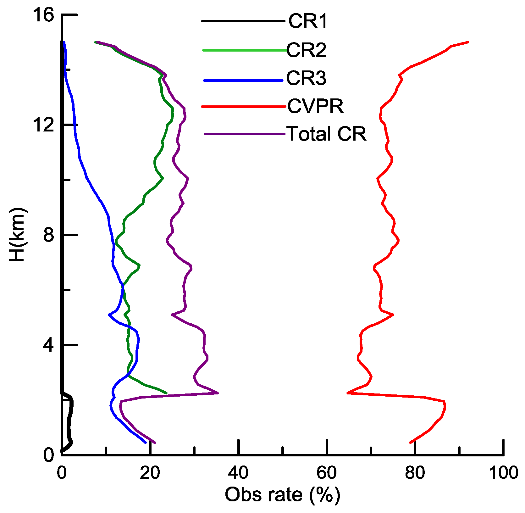
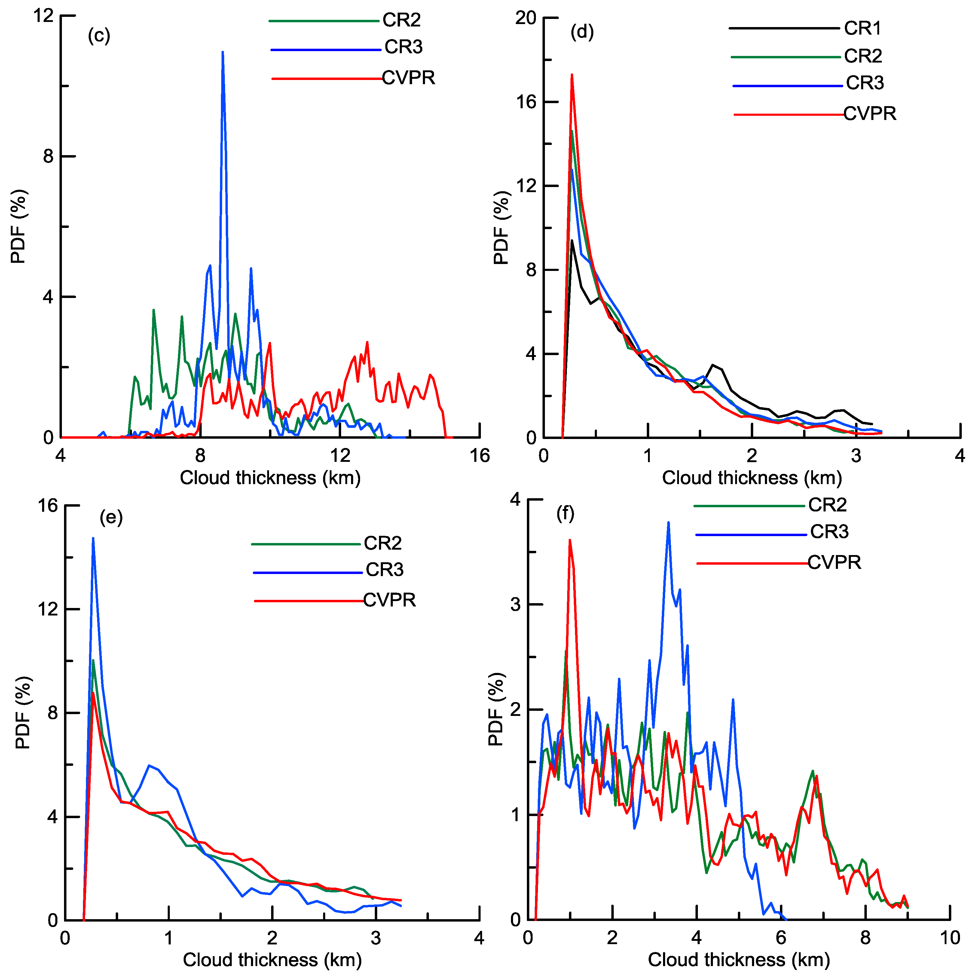
3.2.1. Consistency of CR Modes and CVPR Observations

Reflectivity and velocity biases between the CR modes must be analyzed before merging the data. We present two-dimensional number-of-occurrence histograms of reflectivity and velocity measured by the CR three modes from 1 to 31 July 2016 (in Figure 6). CR3 data are treated as “true” values in the comparison between CR modes, as data from this mode are less affected by coherent integration and pulse compression. High occurrences of reflectivity occur below the diagonal for the CR1 and CR3 modes with a displacement of about 2 dB (Figure 6a) and the CR1 mode tends to underestimate the reflectivity by about 2 dB. However, in the region with strong reflectivity, the occurrence distribution pattern shifts away from the diagonal, which due to the benefit of coherent integration in the CR1 mode is less than the theoretical value. The two-dimensional number-of-occurrence histograms for reflectivity from the CR2 and CR3 modes (Figure 6c) indicate that the high occurrence area occurs above and parallel to the diagonal with a displacement of 2 dB, suggesting that the CR2 mode overestimates the reflectivity by about 2 dB. The two-dimensional number-of-occurrence histograms for velocity (Figure 6b,d) show that the radial velocities measured by the three modes agree very well when the absolute values of the radial velocities are smaller than CR1’s Nyquist velocity.
To assess the consistency between the CR and CVPR observations, we sub-sampled the CVPR reflectivity and velocity to the CR time-height grid for the period of 1 July 2016 to 31 July 2016. For each grid point, we bin the CVPR reflectivity and velocity at 1 dB and 0.5 m·s−1, respectively, together with the corresponding CR3 reflectivity, if detected by both, to form two-dimensional histograms (Figure 7). The intervals for reflectivity and radial velocity were 1 dB and 0.5 m·s−1, respectively.
According to statistical analysis of the raw reflectivity pairs from CR3 and CVPR data taken during July, the averaged raw reflectivities from the CR3 and CVPR are −0.97 and 3.85 dBZ, respectively and the attenuation corrected averaged value from CR3 is 0.28 dBZ. These results suggest that the averaged difference between the CR3 and CVPR measurements is reduced to 4.54 dB from the original 4.82 dB.
For the raw reflectivity, high occurrences of reflectivity values between −25 and −10 dBZ and radial velocity were distributed diagonally, suggesting that no systematic biases are present in the reflectivity and velocity observations from the CR3 and CVPR. However, the occurrence distributions for reflectivities stronger than −10 dBZ were not symmetric about the diagonal, as the CVPR reflectivity values were higher than those from CR3. The high-occurrence areas at −5 and 10 dBZ had displacements of 2 and 4 dB, respectively. The CR3 attenuation corrections reduced the reflectivity bias.

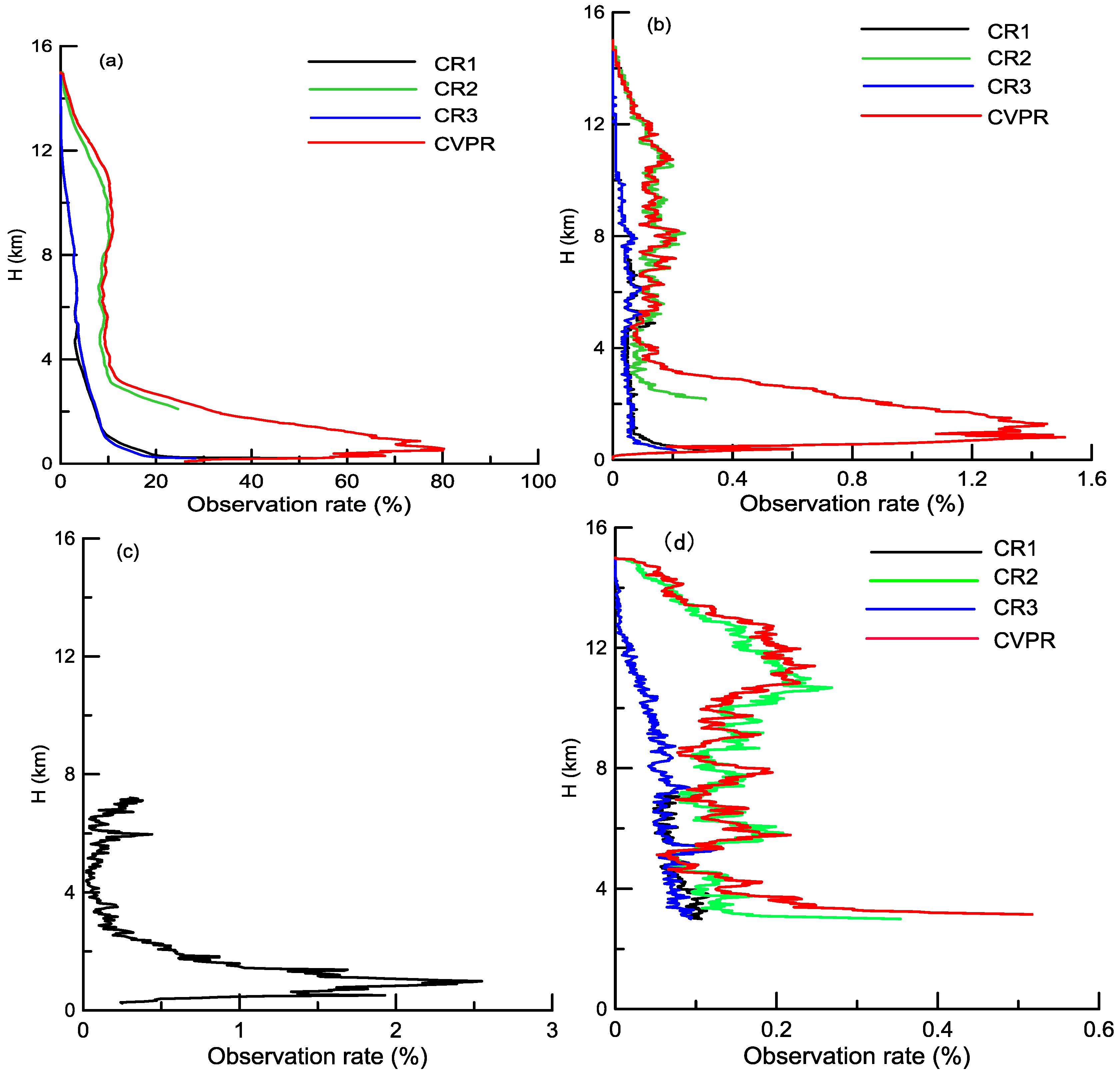
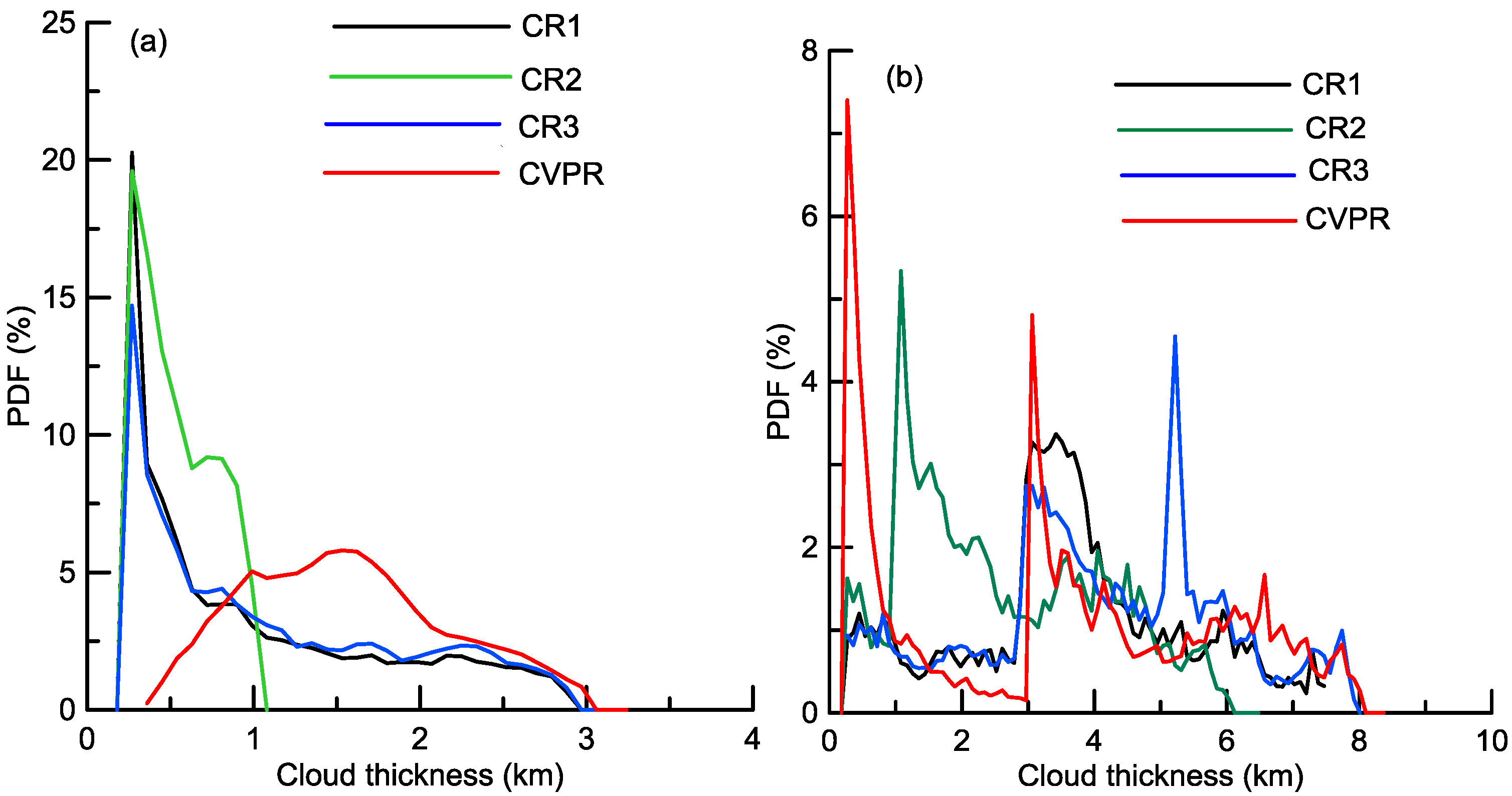
3.2.2. Hydrometeor Observation Statistics

In this study, the valid observation rate is defined as the ratio of the number of valid radar observations to the number of total observations at a certain altitude. A higher observation rate indicates better detection ability. The valid observation rate is related to the minimum reflectivity, radar signal attenuation and hydrometeor reflectivity distributions. Figure 8 shows the valid observation rates, echo base and top rates of CR and CVPR and cloud base rate by CEIL at various altitudes during the period of 1–31 July 2016. Cloud echo is defined as a segment with segment length than 120 m, apart from adjacent segments farther than 60 m, while the upper and lower boundaries of the segment measured by radar were taken as the echo top and base, respectively. In South China, occurrences increased below 3-km altitude, at least 25% of the time, when we observed valid echoes at this level. Few clouds were found between 4 and 6 km altitudes, while large amounts of clouds were concentrated at levels below 3 km and between 8 and 10 km. A similar phenomenon was found over the Tibetan Plateau in summer, where the level with few clouds was located 9.5 km above sea level [20]. Compared to CR1 and CR3, CR2 observed cloud occurrences more than twice as much as did CR1 and CR3. The largest differences between CR1 and CVPR occurred below 2.1 km. The lower valid observation rates and echo base rates of CR were caused by this system’s higher minimum detectable reflectivity relative to CVPR, though some of the observation by CVPR are Bragg scattering. Above 2.1 km, CR2 detection rates agree very well with CVPR detection rates.
The CVPR, CR2 and CEIL systems catch similar profiles of echo/cloud bases above 3.5-km altitude (Figure 8b,c). This suggests that the CVPR, CR2 and CEIL systems have similar capacity for detecting mid-level non-precipitating clouds (cloud base between 3 and 8-km). CEIL observed a maximum cloud base rate of 2.5% at 1.0-km altitude. Although most of time the CVPR observed continuous echoes in vertical direction below 3-km, the echo bases were detected at 0-km height. In addition, CEIL observed cloud bases within precipitation, when echo bases by radars were 0-km. For echo tops, the increased observation rate was occurred at 5.0-km and 8.0-km altitudes. Above 7.0-km height, profiles were shifted 1 km vertically between the CR2 and CVPR data, suggesting that the CR2 underestimated the echo tops due to signal attenuation in precipitating clouds.
Numbers of occurrences of reflectivity at various heights are shown in Figure 9. Above the bright band (about 5 km), CR2 and CVPR observed similar patterns in numbers of occurrences between −20~5 dBZ. The reflectivity in high-occurrence areas decreased with height. However, CR2 could observe weaker clouds with reflectivities <−20 dBZ above 10 km and CVPR observed clouds with reflectivities stronger than 15 dBZ near the bright band. The upper boundary of the minimum contour at 10 dBZ for CVPR is about 2 km higher than the upper boundary for CR2. Below the bright band, the largest differences in numbers of occurrence are located in areas with reflectivities weaker than −15 dBZ or stronger than 20 dBZ. This suggests that Bragg scattering is the main limitation on the use of CVPR data for boundary cloud detection and signal attenuation limited the use of CR for heavy precipitation observations. Comparing CR1, CR2 and CR3, we found that numbers of occurrences of reflectivity weaker than −10 dBZ below 3 km agree well for CR1 and CR3, while CR1 observed more valid data. The high occurrence areas range between 10 and 20 dBZ for CR2 and CR3 near 3-km, while the CR1 occurrences show a 5 dBZ shift to the left. This suggests that coherent integration underestimates the reflectivity of precipitating clouds.
To evaluate the hydrometeor detection capabilities of CR and CVPR, hydrometeors are separated into precipitating and non-precipitating clouds, each of which are subdivided into three categories (precipitating: shallow, congestus and deep clouds; non-precipitating: midlevel, cirrus and anvil clouds) based on their echo base and top heights [10]. In this study, continuous segments with more than 120 m of valid signals were taken as clouds and the boundary was taken to be the echo base/top. Figure 10 shows the mean frequency of observed cloud types from CR three modes and CVPR during July 2016. Note that the sum of all cloud types exceeds 100% because at each given time, multilayered clouds could be present and may be counted in both categories. Among precipitating clouds, the largest differences in frequency occur with shallow clouds. CVPR overestimated shallow cloud frequency compared to CR1 and CR3. This suggests that Bragg scattering is main limitation for the use of CVPR in correctly detecting shallow clouds. For non-precipitating clouds, the CVPR observed frequency agrees very well with CR2, while CR3 detects significantly less mid-and upper-level clouds due to its lower sensitivity.
Cloud thickness is defined as the distance between echo top and base and therefore for precipitating clouds, the thickness includes the precipitation below the actual cloud base by CEIL. The cloud thickness distribution for precipitating clouds and non-precipitating clouds by CR and CVPR were analyzed independently (Figure 11). The CR1 results were not included in deep precipitating clouds and cirrus non-precipitating clouds due to the maximum detectable range. CR2’s minimum detectable range also affected the cloud thickness for precipitating clouds. For shallow clouds, large differences in cloud thickness between CR1, CR2 and CVPR are produced by Bragg scattering of CVPR signal and the minimum detectable reflectivity values. Most of the CVPR detected precipitating shallow clouds may be fog or Bragg scattering echo. Congestus cloud thickness distributions have two peak values at 1 km and 3.5 km by CR1, CR3 and CVPR data, while the CR2 thickness distribution is shifted by 2-km, due to CR2’s minimum detectable range. Most deep precipitating clouds are thicker than 8 km by CR and CVPR; however, CVPR catches a higher frequency of clouds that are thicker than 12 km compared with CR2, likely due to signal CR attenuation in the thick clouds. CR2 reports a much higher frequency of deep cloud thicknesses less than 8 km and CR2 observed thickness distribution is shifted by 2-km compared with CR3 and CVPR due to CR2’s minimum detectable range. For non-precipitating midlevel and cirrus clouds, CR and CVPR report similar patterns of thickness distributions and thickness also follows an exponential distribution falling off quickly above 0.5 km. For anvil clouds, thickness distributions in CR2 and CVPR data agree very well, while CR3 reports higher frequency at 3 km.
This comparison of cloud thickness suggests that the Bragg scattering of CVPR signal in low level, CR signal attenuation in deep precipitation and the minimum detectable range for CR2 are the important issues in merging these data types.

3.3. Quantitative Assessment of the Merged Cloud-Precipitation Data

Figure 12 presents the time-height cross-sections of merged reflectivity and velocity after clutter is removed and these data sources on 4 June 2016. It is evident from Figure 12a that more clouds and precipitation were detected by the merged reflectivity data set, especially for weak clouds and heavy precipitation. Velocity aliasing was not found in the merged velocity series (Figure 12b). The merged echoes below 2.1 km and strong echoes mostly came from CVPR and CR3 data, while weak cloud echoes at the mid- and high-levels were from CR2 data (Figure 12c). Only limited echoes came from CR1 data below 2.1 km, due to velocity folding and underestimated reflectivity.
Figure 13 shows the number-of-occurrences of merged reflectivity. Comparison of Figure 9a,b and c and Figure 13 reveals that merging CVPR data with CR data improves the observation ability for deep precipitating clouds, non-precipitating cirrus clouds with echo tops higher than 8 km and heavy precipitation with reflectivity stronger than 20 dBZ.
The percentages of contributions from the CR1, CR2, CR3 and CVPR data to the merged data are given in Figure 14, showing that the total contribution from all of three CR modes was above 15% below 2.1 km and 30% above 2.1 km. In Guangdong Province, the majority of clouds during the observation period were precipitating convective clouds, which produced severe signal attenuation of CR and favored the usages of the CVPR data, which explains this discrepancy.

3.4. A Statistical Analysis of Merged Cloud and Precipitation Data

In this section, we analyze the diurnal variations of occurrence frequency of the valid merged reflectivity and the averaged reflectivity at various altitudes during July 2016 using the merged data set (Figure 15). Figure 15 makes evident that clouds over South China are distributed widely below 12 km and cloud above 12 km occurred less than 1.0% of the time. The three periods of high occurrence frequency for lower-altitude echoes were 0500–0630, 1000–1230 and 1930–2030 BT. These three periods correspond to local sunrise (0545 BT), noon (1228 BT) and sunset (1910 BT). The development of low-level clouds is often associated with radiative heating and cooling at the surface. Low-altitude clouds that occur at sunrise have weak averaged reflectivity and do not develop further into strong convective clouds. They gradually disappeared after 0700 BT. After 0900 BT, low-level clouds began to form again in greater numbers. Meanwhile, regions of high occurrence of mid- and high-level clouds gradually expanded upward, corresponding to larger averaged reflectivities. By 1400 BT, high occurrence of clouds and precipitation and strong reflectivity (Figure 15a,b) was located at the height of 5–6 km and these clouds basically disappeared by 1600 BT. The temporal evolution of this process indicates that low-level clouds gradually developed into mid- and high-level clouds during this period. After 1600 BT, another precipitation process tended to start. At around 1800 BT, most clouds occurred at 10 km altitude and the corresponding averaged reflectivity reached to 10 dBZ. During 0100–0500 BT, the occurrence frequencies of clouds and precipitation in the mid- and high-level and the corresponding reflectivity values were relatively low. A bright band was observed at 6 km altitude (Figure 15b).
The occurrence frequencies of cloud-base/cloud-top heights are defined as the ratio of their observed times of occurrence at a certain height and temporal grid to the total observation time. Figure 16 shows the diurnal variations of occurrence frequency of cloud-base heights from the merged data and CEIL and cloud-top height from the merged data. We can see from comparing Figure 16a,b that the merged data missed some of mid- and high-level clouds during 0000–1200 BT, which were possibly weak and thin clouds. Results for mid- and high-level clouds by the merged data in the afternoon were consistent with CEIL observations. However, clouds with cloud-base heights above 7 km, which often occurred in the afternoon, were missed from the CEIL observations. Due to the influence of Bragg scattering, fog and precipitation, there existed some differences in the occurrence frequency of low-level clouds observed by radars and CEIL.
The vertical distributions of cloud-base and cloud-top heights are clearly stratified. Few cloud bases were found between 3-km and 5-km height, while large amounts of cloud bases were concentrated at altitudes below 3 km and between 6 and 10 km. This does not mean that a few clouds were found between 3 and 5 km. Clouds with high bases and high tops developed rapidly at altitudes above 5 km after noon time, especially from 1400 BT to 2400 BT.
Figure 17 shows the occurrence frequency distributions of the three types of clouds based on radar observations and the CEIL data. Results from the CEIL observations (Figure 17b) suggest that low-level clouds abruptly dissipate after 0600 BT and then form again during 0700–0900 BT and abruptly increase after 1800 BT. This result agrees very well with changes in the occurrence frequency of low-level echoes, which mainly reflects the influence of solar radiation. CEIL observations indicate that mid- and high-level clouds abruptly increase at the sunrise and this abrupt change was not detected by radars. However, radar observed that the high-level clouds increased abruptly after 1200 BT, which was missed by the CEIL. Radar observed less mid- and high-level clouds than did CEIL.
Comparing the cloud occurrence frequency over Tibetan Plateau in summer [20], the mid- and high-altitude clouds in South China developed relatively early in the day and the cloud occurrence frequency reached a maximum of 2.5% at 9 km altitude between 1200 and 2000 BT (Figure 15a). Clouds over the Tibetan Plateau develop rapidly in the afternoon and reached a maximum of occurrence frequency (50%) during 1800–0400 BT at altitudes between 10.5 and 13.5 km. For both of these areas, the vertical distributions of cloud bases and cloud tops were clearly stratified. Few clouds were found at levels between 3 and 5 km over South China and between 9 and 10 km over the Tibetan Plateau.
To evaluate the vertical distributions of different clouds and precipitations, radar echoes were separated into precipitating and non-precipitating clouds. Non-precipitating clouds are subdivided into three categories (low-, mid- and high-level clouds) based on their cloud bases. Precipitating clouds are subdivided into stratiform and convective precipitation. Segment of the radar beam with cloud base less than 3 km, echo thickness larger than 3 km and maximum reflectivity strong than 5 dBZ were classified as for precipitation echoes, which then were further divided into convective and stratiform precipitation echoes according to the bright bands identified by reflectivity and radial velocity profilers. Figure 18 shows the normalized contoured frequency by altitude diagrams (CFADs) of merged reflectivity for the two types of precipitation and three types of non-precipitating clouds. Vertical profiles of the averaged reflectivity are given in Figure 19, showing that the reflectivity for high-level clouds were within −25~−5 dBZ (Figure 18a) and the averaged reflectivity is about −12 dBZ (Figure 19a), while for mid-level clouds these values were mostly less than −10 dBZ below the height of 7 km. Above this level, most reflectivity were within −10 dBZ to 4 dBZ, a high frequency of mid-level clouds appears at 0 dBZ and 8 km (Figure 18b) and the maximum averaged reflectivity appears at the altitude of 9 km (Figure 19a). The reflectivities for low-level clouds at two high frequency altitudes (at 1.5 and 7.5 km) are −25 dBZ and −10 dBZ, respectively (Figure 18c). The features of upward particle growth below 5 km in low- and mid-altitude non-precipitating clouds are due to the condensation processes driven by uplifting air until the small cloud droplets become embryos of drizzle (Figure 18b,c and Figure 19a). Large reflectivities between 5 and 8 km especially in mid-level clouds indicate remaining hydrometeors suspended in the clouds. The reflectivities above 8 km, on the contrary, tend to decrease gradually with increasing height, likely due to the sublimation or evaporation processes induced by entrainment that often occurs in the vicinity of cloud top. In addition, the reflectivities decrease to less than −15 dBZ near the surface, which are mostly contributed by radiation fog in the morning. The reflectivities also show a great dispersion below 2 km and we speculate the existence of both downdrafts and updrafts over land, causing a region of stronger mixing with wide or irregularly shaped cloud droplet spectra.
Most of the reflectivities for convective and stratiform precipitation were within the ranges of −15~30 dBZ and −15~20 dBZ, respectively. The reflectivities of high occurrence frequencies for convective and stratiform precipitation decreased with altitude significantly between bright band at 5 km and 11 km (Figure 18d,e). Figure 19b shows that the averaged reflectivity of 17 dBZ at 5 km decreased to 5 dBZ at 10 km for convective precipitation, while for stratiform precipitation, the variation of the averaged reflectivity with height is not obvious. The reflectivity values tend to increase monotonically with height from cloud top in precipitation clouds and generally reaches ~20 dBZ in convective areas and ~5 dBZ in stratiform areas at about 5 km altitude, respectively. This trend reflects the downward growth of ice particles by aggregation of hydrometeors or rimming of supercooled cloud water in the upper part of cloud layers. While below 5 km, where the liquid raindrops dominate the radar backscattering signals, the reflectivity distributions are relatively uniform with height, it suggests that the DSDs in the low levels are mainly determined by a balance between collision-coalescence and breakup processes of raindrops.

4. Discussion

The factors causing the differences in reflectivity and velocity between CR and CVPR data include Mie scattering, attenuation, different beam widths and range sidelobe. The ratios of both normalized backscattering cross sections of raindrops and ice spheres for C- and Ka-bands are shown in Figure 20. The differences in reflectivity between data from C- and Ka-band radar are calculated from the raindrop size distributions (DSD) by the disdrometer during July 2016 (Figure 21). Reflectivity for liquid hydrometers by CVPR are weaker than that by CR when D is small (D < 0.3 cm) but in other conditions, CVPR can get stronger reflectivity. For solid ice particles, CVPR can observe stronger reflectivity than that by CR. From the DSD results, the difference of reflectivity by both of bands is less than 2 dBZ.
Aside from Mie scattering and the CR attenuation, beam widths and range sidelobe can introduce reflectivity and velocity biases between the CR and CVPR. The CVPR often observed larger reflectivity below the reflectivity centers, which is possibly due to range sidelobe effects. In the regions with strong reflectivity gradients, differences in reflectivity and velocity are due to the smoothing effects of CVPR’s wide beam width.

5. Conclusions

In this study, Clouds and precipitation data from CR, CVPR, CEIL and microwave radiometer were analyzed to reveal the differences in observations of reflectivity, radial velocity and cloud-base height and to analyze the characteristics of echoes below the CEIL-derived cloud base. A data merging algorithm was then developed to merge observations from the two types of radars and CEIL. Cloud echo base, thickness, frequency of observed cloud types and reflectivity vertical distributions were analyzed in South China. The major conclusions are given as follows.
(i)
The cloud radar with a solid-state transmitter used three operational modes with different pulse widths and coherent and incoherent integrations and realized the minimum detectable reflectivity of −35 dBZ at 5 km and a minimum detection range of 0.2 km. The pulse compression and coherent and incoherent integration in CR1 and CR2 mode can effectively improve the detection ability and introduce reflectivity biases less than 2 dB. The CVPR working in FMCW mode, with two antennas and two-dimensional FFT signal processing technology improved the observation sensitivity. The averaged difference between the attenuation-corrected CR3 and CVPR measurements is reduced to 3.57 dB from the original 4.82 dB. There is no obvious reflectivity bias between CR3 and CVPR (less than 2 dB) for reflectivity weaker than 0 dBZ.
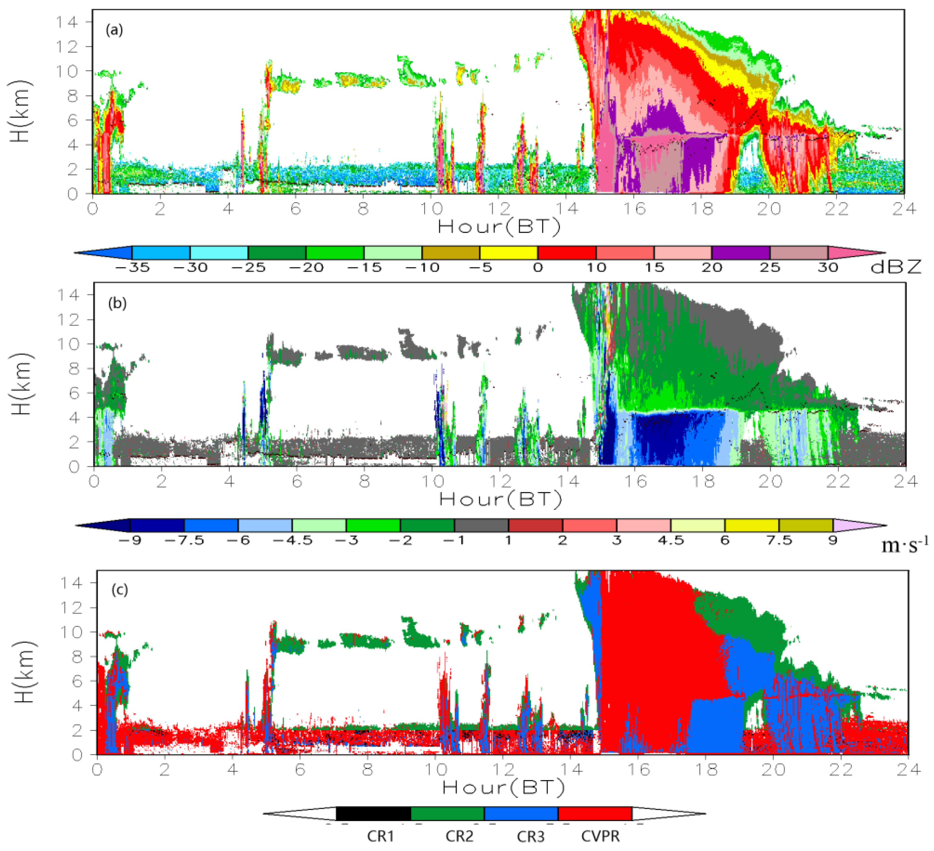
(ii)
The merging CVPR and CEIL data to CR data is to supplement CR deficiency and improve its cloud detection capability for deep cloud. The merged CR, CVPR and CEIL data provides a more complete time-height evolution of the reflectivity and velocity profiles of cloud and precipitation systems, which can fill in the gaps from CR measurements during periods of heavy precipitating and improve CVPR measurements in the boundary layer. At same time, the merging of velocity data with different Nyquist velocities and resolutions diminishes velocity folding, providing more fine information about cloud and precipitation dynamics. This merged dataset can be used to improve our understanding of the microphysical properties and dynamics of cloud and precipitation systems.
(iii)
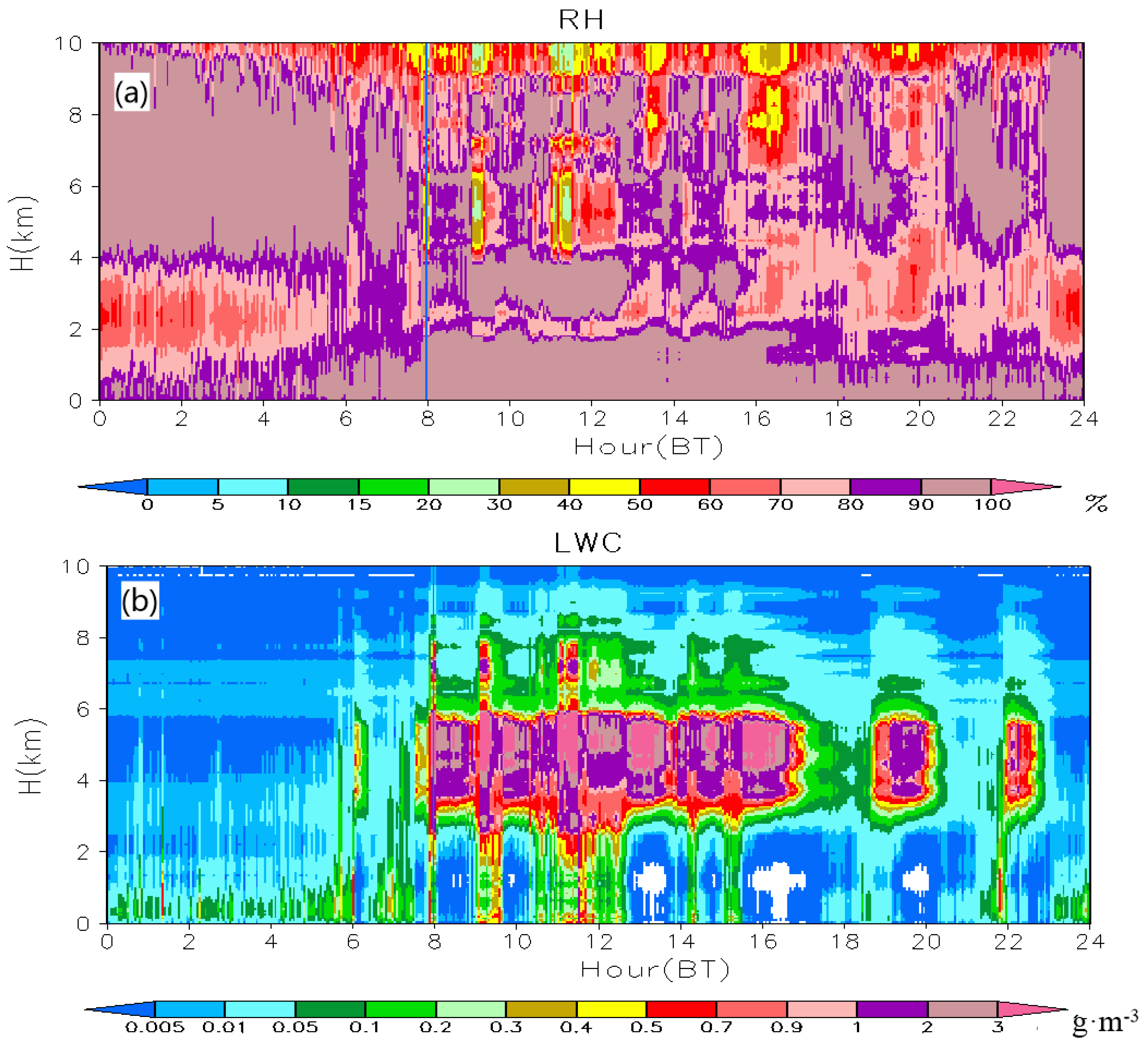
Echoes in PLB observed by CVPR and CR1 correspond to RH more than 80% and valid LWC. These facts suggest that when cloud or fog are in PBL, Bragg scattering and the high sensitivity of the CVPR made it detect more echoes. In this case, comparison with CEIL, CR and CVPR failed to detect cloud in PBL. On the contrary, CR2 and CVPR observed similar cloud occurrences above 4 km and their echo base distributions are similar to those from CEIL. CVPR, CR2 and CEIL therefore have similar observation capabilities for mid-level and high-level non-precipitating clouds.
(iv)
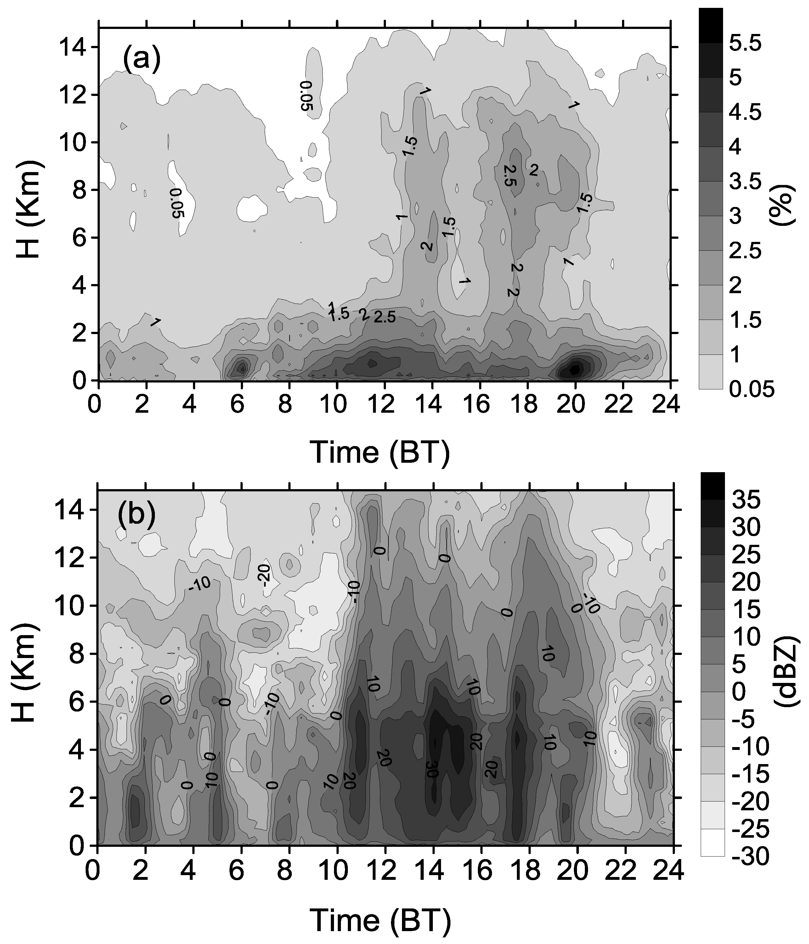
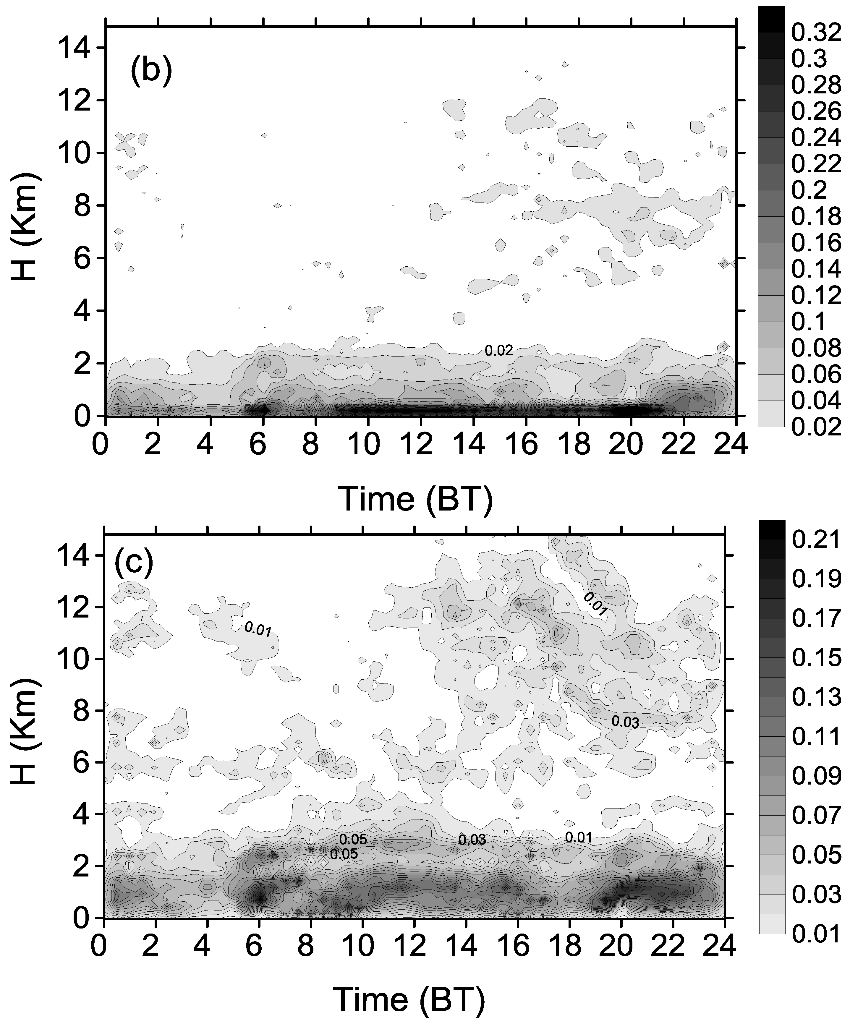
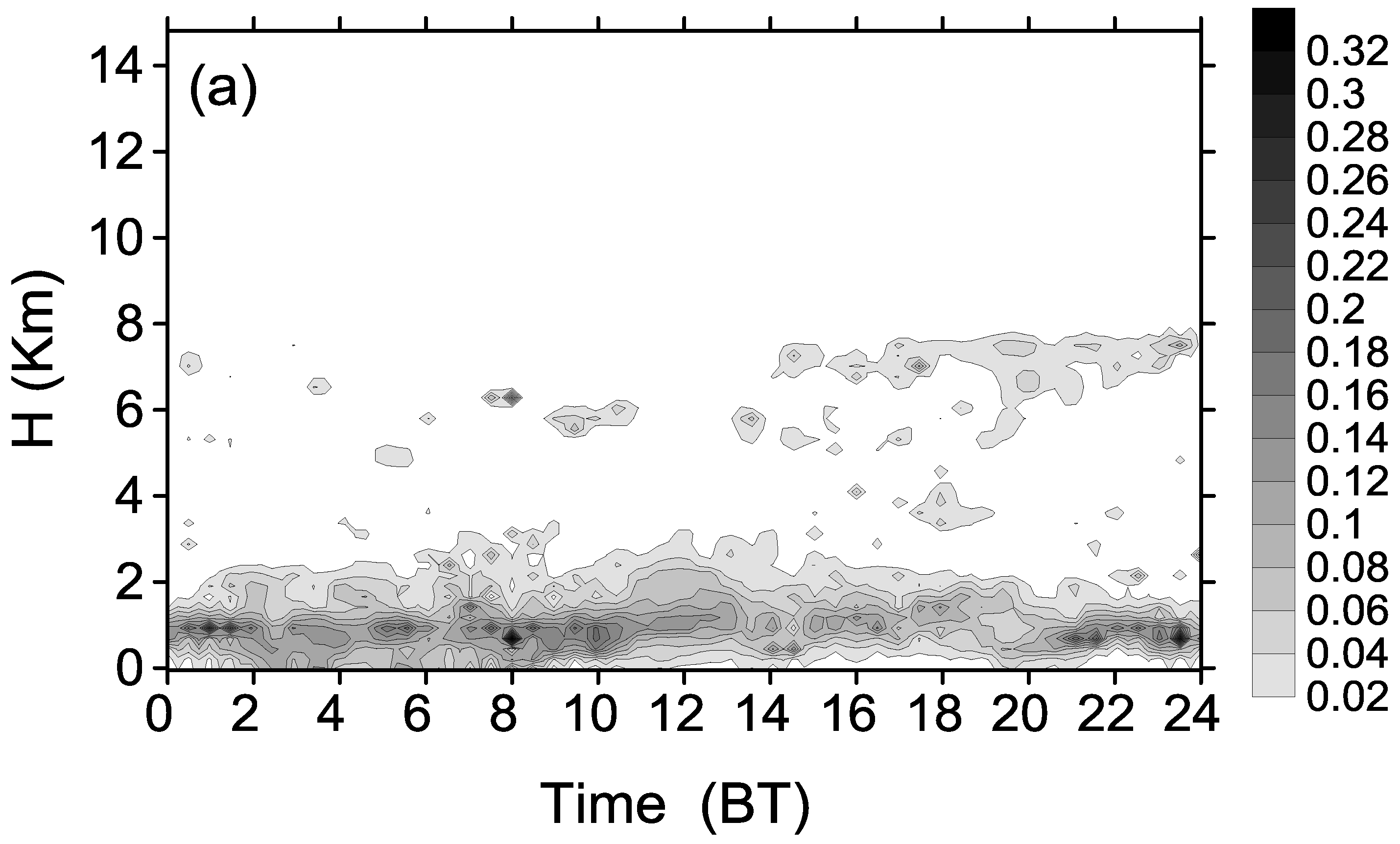
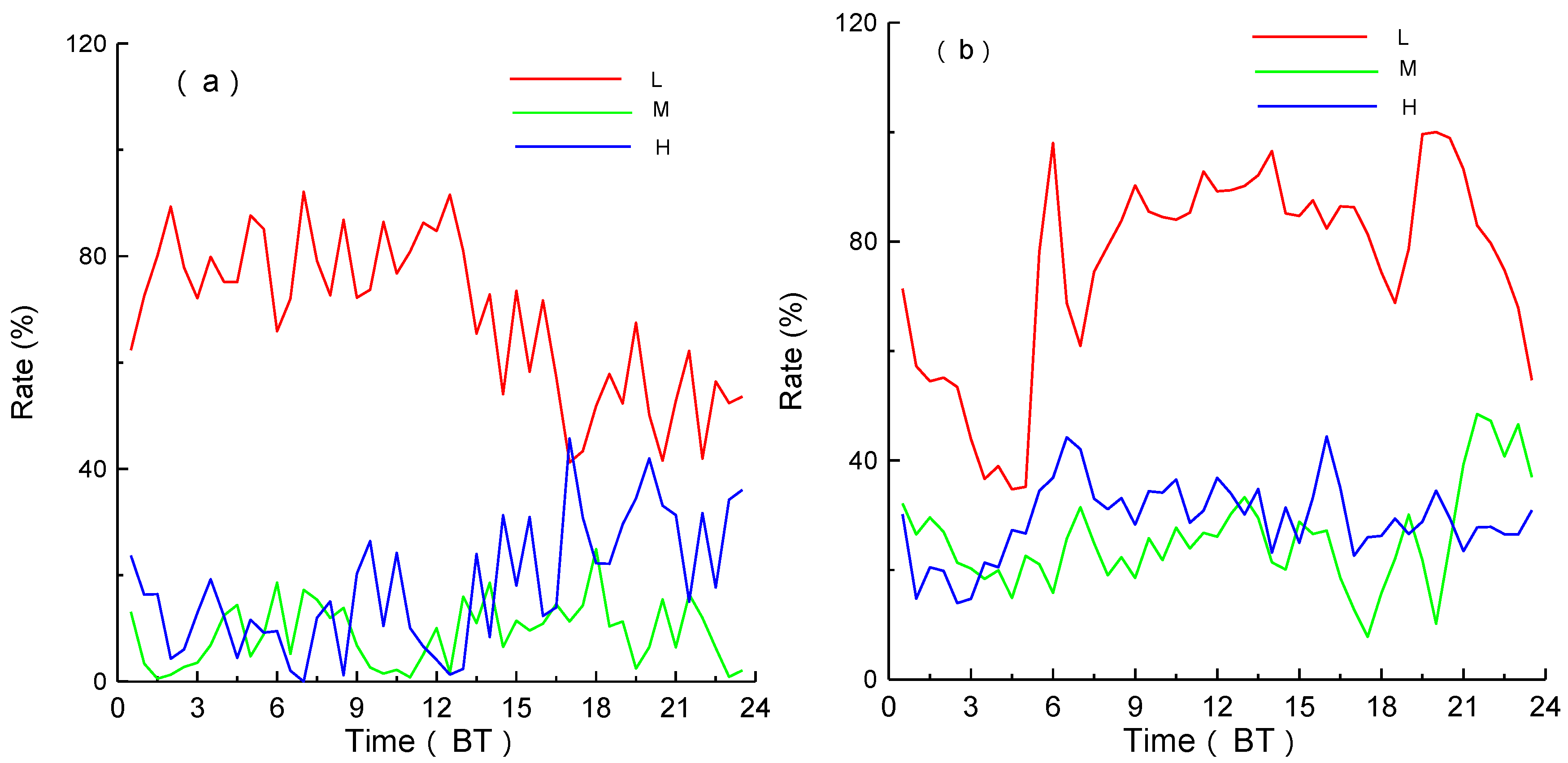
The three periods of high occurrence frequency of low-level clouds occurred at sunrise, noon and sunset and large differences in the average reflectivity could be found. Two high occurrence frequency periods for mid- and high-level clouds occurred at 1400 BT and 1800 BT. Few clouds were found between 3 km and 5 km altitude, while large amounts of clouds were concentrated at levels below 3 km and in the layer between 6 and 10 km. Diurnal variations of cloud occurrence frequency and their vertical distributions for South China and the Tibetan Plateau were different. However, there are obvious levels with few clouds in both areas.
(v)
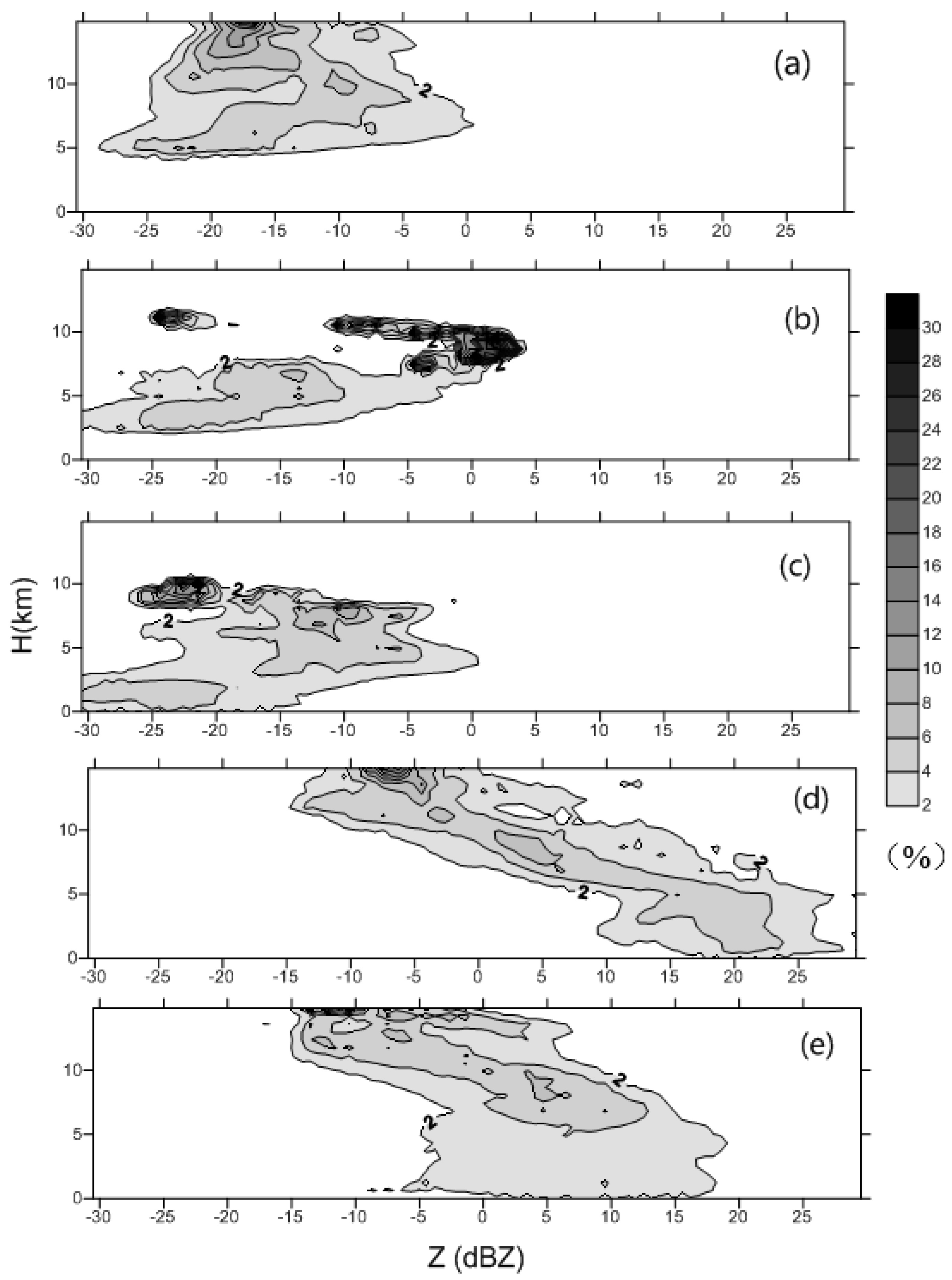
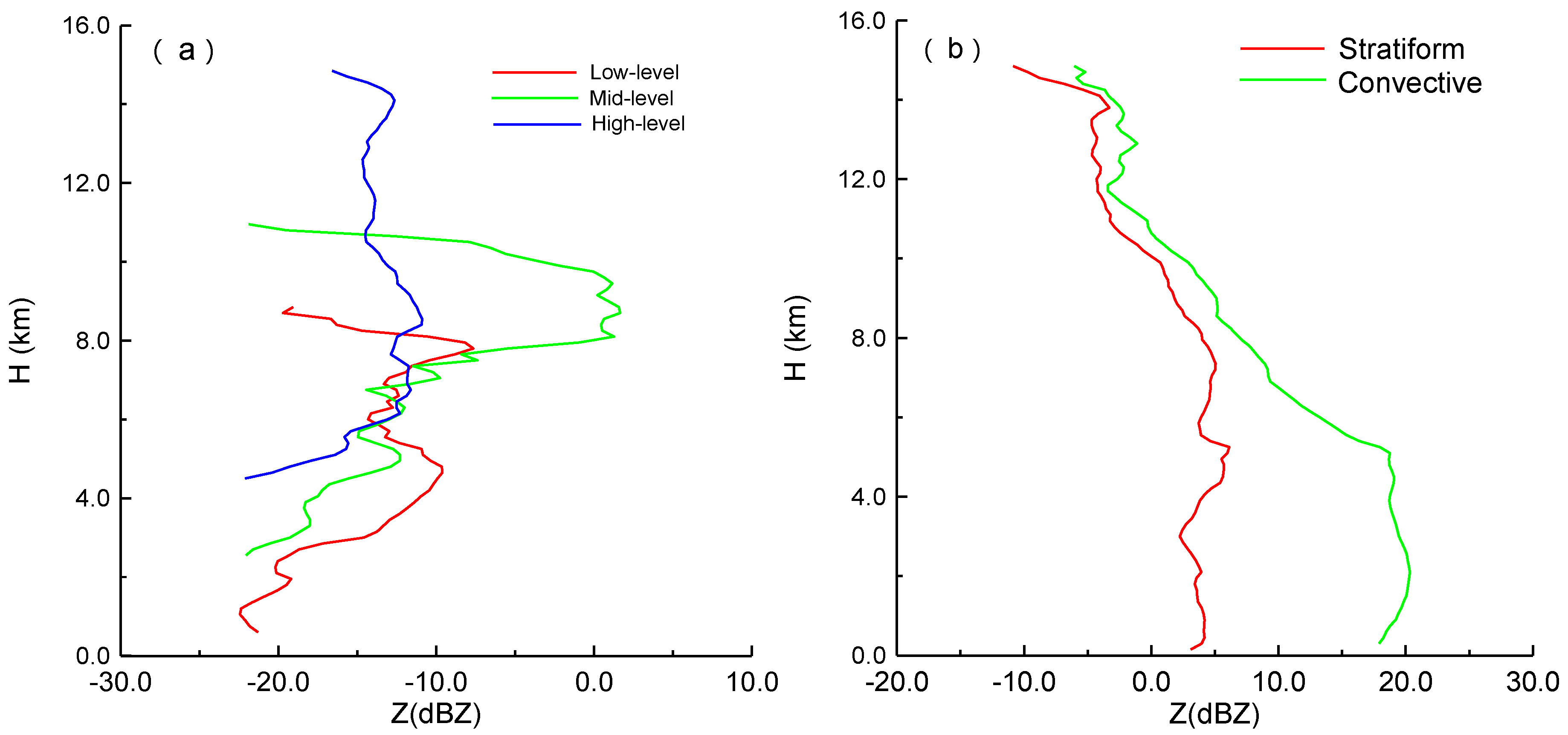
Low-level and high-level clouds have similar averaged reflectivity of about −10 dBZ, while, the averaged reflectivity for mid-level clouds are relative strong (about 0 dBZ). The variations of reflectivity distributions with altitude for stratiform and convective precipitations above 5 km are different, which reveal that different micro-physical processes occur in the two types of precipitation systems.

Acknowledgments

This work was jointly funded by the National Natural Science Foundation of China (41675023, 91337103, 91437101, 41475029 and 41705008 ), Scientific Research Projects of the Chinese Academy of Meteorological Sciences (CAMS) (2016Z005). Thanks to Dalin Zhang in University of Maryland, USA, for his English writing revise and suggestions.

Author Contributions

Liping Liu conceived, designed, processed, analyzed and wrote the manuscript; Zheng Ruan and Wenhua Gao conducted CVPR processing and statistical analysis of the clouds and precipitation; Jiafeng Zheng processed the data used in this manuscript.

Conflicts of Interest

The authors declare no conflict of interest.

References

  1. Hartmann, D.L.; Ockert-Bell, M.E.; Michelsen, M.L. The Effect of Cloud Type on Earth’s Energy Balance: Global Analysis. J. Clim. 1992, 5, 1281–1304. [Google Scholar] [CrossRef]
  2. Zhang, J.; Chen, H.; Li, Z.; Fan, X.; Peng, L.; Yu, Y.; Crbb, M. Analysis of cloud layer structure in Shouxian, China using RS92 radiosonde aided by 95 GHz cloud radar. J. Geophys. Res. 2010, 115. [Google Scholar] [CrossRef]
  3. Thurairajah, B.; Shaw, J.A. Cloud statistics measured with the infrared cloud imager (ICI). IEEE Trans. Geosci. Remote Sens. 2005, 43, 2000–2007. [Google Scholar] [CrossRef]
  4. Clothiaux, E.E.; Ackerman, T.P.; Mace, G.G.; Moran, K.P.; Marchand, R.T.; Miller, M.A.; Martner, B.E. Objective determination of cloud heights and radar reflectivities using a combination of active remote sensors at the ARM CART sites. J. Appl. Meteorol. 2000, 39, 645–665. [Google Scholar] [CrossRef]
  5. Huang, X.; Hu, H.; Xia, J.; Bo, L.; Zhang, X.; Lei, Y.; Huang, J.; Wang, W.; Wu, D.; Jiang, C.; et al. Comparison and analysis of cloud base height measured by ceilometer, infrared cloud measuring system and cloud radar (in Chinese with English abstract). Chin. J. Quantum Electron. 2013, 30, 73–78. [Google Scholar]
  6. Tao, F.; Ma, S.; Qin, Y.; Hu, S.; Wen, X.; Lei, Y.; Guo, W.; Zhang, C. Cloud base height measurement methods based on dual-camera stereovision (in Chinese with English abstract). J. Appl. Meteorol. Sci. 2013, 24, 323–331. [Google Scholar]
  7. Gaumet, J.L.; Heinrich, J.C.; Cluzeau, M.; Pierrard, P.; Prieur, J. Cloud-base height measurements with a single-pulse erbium-glass laser ceilometer. J. Atmos. Ocean. Technol. 1998, 15, 37–45. [Google Scholar] [CrossRef]
  8. Moran, K.P.; Martner, B.E.; Post, M.J.; Kropfli, R.A.; Welsh, D.C.; Widener, K.B. An unattended cloud-profiling radar for use in climate research. Bull. Am. Meteorol. Soc. 1998, 79, 443–455. [Google Scholar] [CrossRef]
  9. Clothiaux, E.E.; Moran, K.P.; Martner, B.E.; Ackerman, T.P.; Mace, G.G.; Uttal, T.; Mather, J.H.; Widener, K.B.; Miller, M.A.; Rodriguezand, D.J. The Atmospheric Radiation Measurement Program Cloud Radars: Operational Models. J. Atmos. Ocean. Technol. 1999, 16, 819–827. [Google Scholar] [CrossRef]
  10. Feng, Z.; Sally, A.M.; Courtney, S.; Ellis, S.; Comstock, J.; Bharadwaj, N. Constructing a merged cloud-precipitation radar dataset for tropical convective clouds during the DYNAMO/AMIE experiment at Addu Atoll. J. Atmos. Ocean. Technol. 2014, 31, 1021–1042. [Google Scholar] [CrossRef]
  11. Li, S.; Ma, S.; Gao, Y.; Yang, L.; Pu, X.; Tao, F. Comparative analysis of cloud base heights observed by cloud radar and ceilometer (in Chinese with English abstract). Meteorol. Mon. 2015, 41, 212–218. [Google Scholar]
  12. Yan, B.; Song, X.; Chen, C.; Liu, Z. Beijing atmospheric boundary layer observation with Lidar in 2011 spring (in Chinese with English abstract). Acta Opt. Sin. 2013, 33(S1), s128001. [Google Scholar] [CrossRef]
  13. Cao, N.; Shi, J.Y.; Zhang, Y.; Yang, F.; Jian, L.; Bo, L.; Xia, J.; Yang, J.; Yan, P. Aerosol Measurements by Raman-Rayleigh-Mie Lidar in North Suburb Area of Nanjing City (in Chinese with English abstract). Laser Optoelectron. Prog. 2012, 49, 060101. [Google Scholar] [CrossRef]
  14. Richter, J. High-resolution tropospheric radar sounding. Radio Sci. 1969, 4, 1261–1268. [Google Scholar] [CrossRef]
  15. Eaton, F.D.; Mclaughlin, S.A.; Hines, J.R. A new frequency-modulated continuous wave radar for studying planetary boundary layer morphology. Radio Sci. 1995, 30, 75–88. [Google Scholar] [CrossRef]
  16. Ince, T.; Friasier, S.T.; Muschinski, A.; Pazmany, A.L. An S-band frequency-modulated continuous-wave boundary layer profiler: Description and initial results. Radio Sci. 2003, 38. [Google Scholar] [CrossRef]
  17. Bennett, L.J.; Weckwerth, T.M.; Blyth, A.M.; Geerts, B.; Miao, Q.; Richardson, Y.P. Observations of the evolution of the nocturnal and convective boundary layers and the structure of open-celled convection on 14 June 2002. Mon. Weather Rev. 2010, 138, 2589–2607. [Google Scholar] [CrossRef]
  18. Peters, G.; Fischer, B.; Andersson, T. Rain observations with a vertically looking Micro Rain Radar (MRR). Boreal Environ. Res. 2002, 7, 353–362. [Google Scholar]
  19. Melchionna, S.; Bauer, M.; Peters, G. A new algorithm for the extraction of cloud parameters using multipeak analysis of cloud radar data—First application and preliminary results. Meteorol. Z. 2008, 17, 613–620. [Google Scholar] [CrossRef] [PubMed]
  20. Liu, L.; Zheng, J.; Ruan, Z.; Cui, Z.; Hu, Z.; Wu, S.; Dai, G.; Wu, Y. Comprehensive radar observations of clouds and precipitation over the Tibetan Plateau and preliminary analysis of cloud properties. J. Meteorol. Res. 2015, 29, 546–561. [Google Scholar] [CrossRef]
  21. Liu, L.; Zheng, J.; Wu, J. A Ka-band solid-state transmitter cloud radar and data merging algorithm for its measurements. Adv. Atmos. Sci. 2017, 34, 545–558. [Google Scholar] [CrossRef]
  22. Ruan, Z.; Jin, L.; Ge, R.; Li, F.; Wu, J. The C-band CVPR pointing weather radar system and its observation experiment (in Chinese with English abstract). ACTA Meteorol. Sin. 2015, 73, 577–592. [Google Scholar]
  23. Luo, Y.; Zhang, R.; Wan, Q.; Wang, B.; Wong, W.K.; Hu, Z.; Jou, B.J.; Lin, Y.; Johnson, R.H.; Chang, C.P.; et al. The Southern China Monsoon Rainfall Experiment (SCMREX). Bull. Am. Meteorol. Soc. 2017, 98, 999–1013. [Google Scholar] [CrossRef]
  24. Wu, Y.; Liu, L. Statistical characteristics of raindrop size distribution in the Tibetan Plateau and Southern China. Adv. Atmos. Sci. 2017, 34, 727–736. [Google Scholar] [CrossRef]
  25. Barber, P.; Yeh, C. Scattering of electromagnetic wave by arbitrarily shaped dielectric bodies. Appl. Opt. 1975, 14, 2864–2872. [Google Scholar] [CrossRef] [PubMed]
  26. Wang, Z.; Teng, X.; Ji, L.; Zhao, F. A study of the relationship between the attenuation coefficient and radar reflectivity factor for spherical particles in clouds at millimeter wavelengths (in Chinese with English abstract). Acta Meteorol. Sin. 2011, 69, 1020–1028. [Google Scholar]
Figure 1. Changes in minimum detectable reflectivity as a function of height for CR’s modes (black) and CVPR (red).
Remotesensing 09 01282 g001
Figure 2. Cumulative probability distributions of “clear sky” reflectivity by CR1, CR2, CR3 and CVPR.
Remotesensing 09 01282 g002
Figure 3. The time-height cross-sections of reflectivity on 4 June 2016 from: (a) CR1; (b) CR2; (c) CR3 and (d) CVPR. The block dots are the CEIL-derived cloud-base heights.
Remotesensing 09 01282 g003
Figure 4. The time-height cross-sections of (a) relative humidity (RH) and (b) liquid water content (LWC) from MWR data taken on 4 June 2016.
Remotesensing 09 01282 g004
Figure 5. Time-height cross-sections of radial velocity on 4 June 2016 from: (a) CR1; (b) CR2; (c) CR3 and (d) CVPR.
Remotesensing 09 01282 g005
Figure 6. Two-dimensional number-of-occurrences of reflectivity and radial velocity from observations of (a) reflectivity for CR3 and CR1 in dBZ; (b) radial velocity for CR3 and CR1; (c) reflectivity for CR3 and CR2 and (d) radial velocity for CR3 and CR2.
Remotesensing 09 01282 g006
Figure 7. Two-dimensional number-of-occurrence histograms of reflectivity from observations of (a) raw CR3 and CVPR; (b) corrected CR3 and CVPR; and (c) radial velocity for CR3 and CVPR.
Remotesensing 09 01282 g007
Figure 8. Valid observation rates of (a) valid reflectivity; (b) echo bases by radars and (c) cloud bases by CEIL and (d) echo tops at different altitude.
Remotesensing 09 01282 g008
Figure 9. The numbers of occurrences of reflectivity for (a) CR1; (b) CR2; (c) CR3 and (d) CVPR.
Remotesensing 09 01282 g009
Figure 10. Mean frequency of observed cloud types from CR three modes and CVPR.
Remotesensing 09 01282 g010
Figure 11. Cloud thickness distribution for precipitating clouds: (a) shallow; (b) congestus; (c) deep clouds and non-precipitating clouds; (d) midlevel; (e) cirrus and (f) anvil by CR and CVPR.
Remotesensing 09 01282 g011aRemotesensing 09 01282 g011b
Figure 12. Time-height cross-sections of reflectivity on 4 June 2016: (a) the merged reflectivity and (b) velocity; and (c) data sources for reflectivity and velocity. The black dots in (a,b) indicate the CEIL-derived cloud-base heights. In (c), data from CR1, CR2, CR3 and CVPR are shaded in black, green, blue and red, respectively.
Remotesensing 09 01282 g012
Figure 13. Numbers of occurrences of merged reflectivity.
Remotesensing 09 01282 g013
Figure 14. Percentage contributions from CR1 (black), CR2 (green), CR3 (blue), entire CR (purple) and CVPR (red) to the merged reflectivity.
Remotesensing 09 01282 g014
Figure 15. Diurnal variations of (a) occurrence frequency of valid merged reflectivity and (b) averaged reflectivity at various altitudes during July 2016.
Remotesensing 09 01282 g015
Figure 16. Diurnal variations of occurrence frequency of cloud-base heights from (a) CEIL observation; and (b) the merged data; and (c) cloud-top heights from the merged data.
Remotesensing 09 01282 g016aRemotesensing 09 01282 g016b
Figure 17. Diurnal variations of cloud occurrence frequencies of low-altitude (L in red), mid-altitude (M in green) and high-altitude (H in blue) clouds from (a) the merged data; and (b) the CEIL observations.
Remotesensing 09 01282 g017
Figure 18. Normalized CFADs (%) of reflectivity of non-precipitating and precipitating clouds based on merged data during July 2016: (a) high-level non-precipitating clouds; (b) mid-level non-precipitating clouds; (c) low-level non-precipitating clouds; (d) convective precipitating clouds; and (e) stratiform precipitating clouds.
Remotesensing 09 01282 g018
Figure 19. Vertical profiles of averaged reflectivity for (a) non-precipitating clouds (low-, mid- and high-level) and (b) precipitating clouds (convective and stratiform).
Remotesensing 09 01282 g019
Figure 20. Ratios of corrected backscattering cross sections of raindrops and ice spheres with Ka and C bands (Ka/C).
Remotesensing 09 01282 g020
Figure 21. Two-dimensional occurrences of reflectivity differences by C and Ka band radars from DSD data by the disdrometer.
Remotesensing 09 01282 g021
Table 1. Main technical parameters for the Ka band solid-state transmitter cloud radar.
OrderItemsTechnical Specifications
General Technical Parameter of the Cloud Radar System
1Radar systemCoherent, pulsed Doppler, solid-state transmitter, pulse compression
2Radar frequency33.44 GHz (Ka-band)
3Beam width0.35°
4Detecting parametersZ, Vr, SW, LDR, Sz
5Detection capability≤−30 dBZ at 5 km
6Range of detectionHeight: 0.120 km~15 km
Reflectivity: −50 dBZ~+30 dBZ
radial velocity: 4.67 m·s−1~18.67 m·s−1 (maximum)
velocity spectrum width: 0 m·s−1~4 m·s−1 (maximum)
Temporal resolution: 6 s (adjustable)
Height resolution: 30 m
Table 2. Major operational parameters for the three operational modes.
OrderItemsBoundary Mode (CR1)Cirrus Mode (CR2)Precipitation Mode (CR3)
1the pulse width0.2 μs12 μs0.2 μs
2the pulse repetition frequency8333 HZ8333 HZ8333 HZ
3the number of coherent integration421
4the number of incoherent integration163264
5the number of fast Fourier transform points256256256
6Dwell time2 s2 s2 s
7the number of range gates256, 128512, 256512, 256
8the range sample volume spacing30 m30 m30 m
9the minimum range30 m (theoretical)1800 m (theoretical)30 m (theoretical)
120 m (practical)2010 m (practical)120 m (practical)
10the maximum range18 km18 km18 km
11Nyquist velocity4.67 m·s−19.34 m·s−118.67 m·s−1
12the radial velocity resolution0.018 m·s−10.036 m·s−10.073 m·s−1
Table 3. Main technical parameters of the C-FMCW radar system.
OrderItemsTechnical Specifications
1Radar systemfrequency modulated continuous wave, vertically pointing
2Radar wave frequency5530 MHz
3AntennaDouble Parabolic, Two antennas for transmitting and receiving, Beam width 2.6°
4Range of detection0.1–24 km (vertical direction)
5Nyquist velocity22 m·s−1
6Dwell time2–3 s
7range solution and gate numberrange solution: 15 m, 30 m; Gate number: 512, 1024
8Detecting parametersZ, Vr, SW, Sz
Table 4. Major technical parameters and data for CL51 ceilometer.
OrderItemsTechnical Specifications
1Transmitterpulsed
2Wave length (nm)910 ± 10
3Peak power (W)27
4Pulse repetition frequency (kHz)6.5
5Sampling volume (mm3)834 × 266 × 264
6Detection range (km)0~15
7Cloud Measurable height (km)0~13
8Spatial resolution (m)10
9Temporal resolution6 s
10Vertical visibility (m)Cloud base heights for first, second and third layers (m)
Table 5. Major technical parameters and data for disdrometer.
OrderItemsTechnical Specifications
1Measurable diameter range (mm)0.062~24.5 mm
2Measurable velocity range (m·s−1)0.05~20.8
3Sensor sampling size (cm2)54
4Temporal resolution (s)60
5Grade number32
6Diameter grades (mm)0.062, 0.187, 0.312, 0.437, 0.562, 0.687, 0.812, 0.937, 1.062, 1.187, 1.375, 1.625, 1.875, 2.125, 2.375, 2.75, 3.25, 3.75, 4.25, 4.75, 5.5, 6.5, 7.5, 8.5, 9.5, 11, 13, 15, 17, 19, 21.5, 24.5
7Velocity grades (m·s−1)0.05, 0.15, 0.25, 0.35, 0.45, 0.55, 0.65, 0.75, 0.85, 0.95, 1.1, 1.3, 1.5, 1.7, 1.9, 2.2, 2.6, 3, 3.4, 3.8, 4.4, 5.2, 6.0, 6.8, 7.6, 8.8, 10.4, 12, 13.6, 15.2, 17.6, 20.8
8Rain amount (mm)1 min, 1 h
9Rain rate (m·s−1)1 min, 1 h
10Reflectivity (dBZ) Z = D i = 0 D m a x N ( D i ) D i 6 Δ D (for Rayleigh scattering)

