Estimating the Rut Depth by UAV Photogrammetry

Abstract

The rut formation during forest operations is an undesirable phenomenon. A methodology is being proposed to measure the rut depth distribution of a logging site by photogrammetric point clouds produced by unmanned aerial vehicles (UAV). The methodology includes five processing steps that aim at reducing the noise from the surrounding trees and undergrowth for identifying the trails. A canopy height model is produced to focus the point cloud on the open pathway around the forest machine trail. A triangularized ground model is formed by a point cloud filtering method. The ground model is vectorized using the histogram of directed curvatures (HOC) method to produce an overall ground visualization. Finally, a manual selection of the trails leads to an automated rut depth profile analysis. The bivariate correlation (Pearson’s r) between rut depths measured manually and by UAV photogrammetry is $r=0.67$. The two-class accuracy a of detecting the rut depth exceeding 20 cm is $a=0.65$. There is potential for enabling automated large-scale evaluation of the forestry areas by using autonomous drones and the process described.

1. Introduction

Mechanized wood harvesting operations can cause rut formation, which deteriorates soil quality, decreases forest productivity and affects hydrological balance and water quality through changed sediment discharge [1,2,3,4,5,6,7,8]. Thus, the rut depth distribution is one of the central measures of the environmental and economic impact of harvesting operations.

Indeed, international forest certification standards issued by the Forest Stewardship Council (FSC) and by the Programme for the Endorsement of Forest Certification (PEFC) along with national legislations have recommendations and regulations concerning the rut formation [9,10]. Monitoring the obedience of standards and laws requires data of ruts, and these data are traditionally collected by manual measurements from randomly-selected samples of logging sites [11]. Due to the costs of time-consuming manual measurements, data collected cover unfortunately only a very small part of the operation sites.

Ruts are formed when the loading exerted by the forest vehicle exceeds the strength of the soil [12,13,14]. The bearing capacity depends on various static and dynamic factors: e.g., soil type, root density, slope and other micro-topographic water dynamics and frost state. As a result, both the spatial and temporal variation in trafficability is extremely large [14,15]. An easily collected and extensive dataset on rut depths that covers field measurements over several test sites and various weather conditions is thus needed for any attempts to model forest terrain trafficability [16].

The development of techniques in the collection, processing and storage of data offers a great possibility to collect extensive datasets on rut formation. Close-range aerial imagery captured by unmanned aerial vehicles (UAV) provides one of several methods under development. This method for retrieving data on changing terrain by photogrammetry with efficient digital workflows has been used by [4,13,17,18].

Other potential methods include light detection and ranging (LiDAR) scanning [16,19] and ultrasonic distance ranging accompanied by proxy measurements such as controller area network (CAN-bus) data [20]. Compared with other methods, UAV photogrammetry provides a cost-effective option for collecting high-resolution 3D point clouds documenting the operation site in full extent [4].

The photogrammetric UAV data have some deficiencies [20] when compared with aerial LiDAR (ALS) [21]. ALS is a true 3D mapping method in the sense that it allows multiple Z returns from a single laser beam, whereas photogrammetric data have only one Z value for each point. This results in hits concentrated at the top layer of the dense canopy or undergrowth, leaving the ground model often rather inadequate or narrow.

Usually, the logging trails have a corresponding canopy opening (a canopy pathway) around them, and the UAV data points sample the trail surface if the flight altitude is low enough and the flight pattern dense enough. Occasional obstructions and discontinuities occur, though, and the numerical methods must adapt to this difficulty. While the point cloud is limited compared to the one produced by a LiDAR scanner, the potential for rut depth detection is worth examining due to lesser costs, smaller storage demands and abundance of details provided by the imagery (RGB) information.

A large dataset on ruts would aid not only extensive monitoring of forest standards, but also the modeling and forecasting purposes as rut formation depends quite directly on soil bearing capacity and, thus, relates to forest terrain trafficability [22]. A post-harvest quality assurance pipeline using the UAV technology could be an essential part in cumulating such dataset.

The rut width depends on the tire dimensions, and the distance between the ruts depends on the forest machine dimensions; these can be approximately known a priori. The rut features have generally a rather fixed scale: a rut is about 0.6–1.2 m wide; the depth varies between 0 and 1.0 m; and the distance between ruts is a machine-specific constant usually known beforehand (approximately 1.8–2.5 m).

The most relevant study in trail detection is [23], where the usage of the digital elevation map (DEM) has been avoided, making the point cloud recording possible without specific geo-referencing markers. This makes the field procedure simpler and faster and gives more freedom to choose the UAV flight pattern. A multi-scale approach similar to [24] could be useful, since the point cloud density changes especially at the canopy border. Now, a mono-scale analysis has been used. The triangularization produced by methods described in Section 2.5 has approximately a 20-cm average triangle edge length.

Several restrictions have been made in [23]: the locations have to be relatively smooth and without underbrush. An interesting study of [4] uses photogrammetric data from a ground-based recording device. A very good matching of rut depth has been achieved using different point cloud processing methods. The test site is open canopy, but measurements require a field team traversing the trail.

We propose a sequence of processing steps for more realistic conditions (varying terrain, some underbrush and trees allowed, trail pathways only partially exposed from the canopy cover). We have subtracted DEM height provided by the National Land Survey of Finland (NLS) for some visualizations, but actual methods are independent of the local DEM.

We propose a procedure for large-scale field measurement of rut depth. The procedure is based on the point cloud collected by the UAV photogrammetry. The following data models are constructed for autonomous logging trail detection and finally for rut depth data extraction:

• a canopy height model to focus the point cloud on the logging trail. The model is produced by a solid angle filtering (SAF) of point clouds [25];
• a surface model as a triangularized irregular network (TIN) for trail detection; the model is produced by applying SAF with a different parameter setting, followed by mean curvature flow smoothing (MCF) [26];
• ground model vectorization (orientation of possible ruts and likelihood of having a trail through any given point;
• the height raster of a straightened harvesting trail; this phase uses a histogram of curvatures (HOC) method;
• a collection of 2D rut profile curves.

2. Materials and Methods

2.1. Study Area

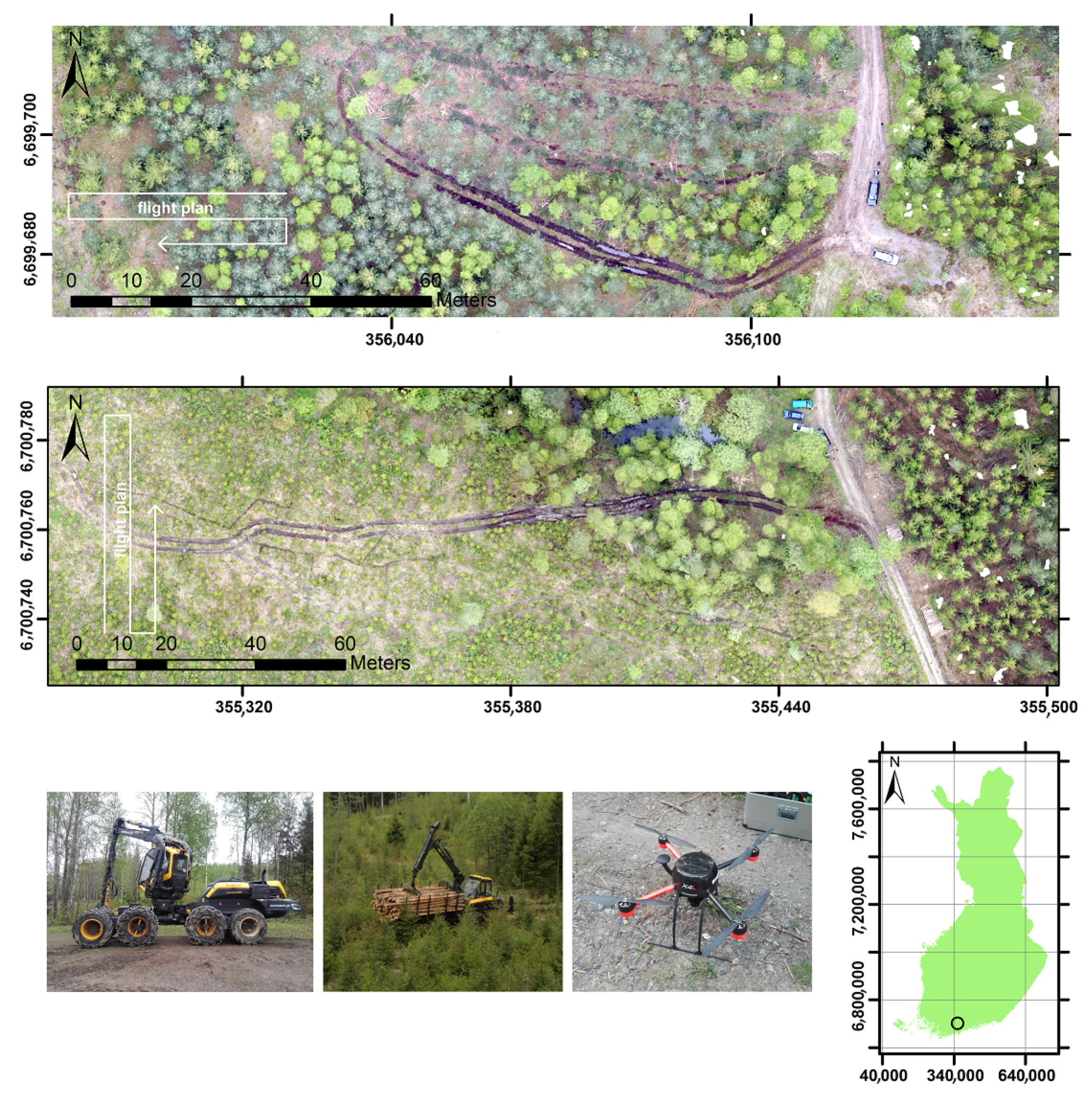
The field study was carried out in Vihti, Southern Finland (60${}^{\circ }$24.48′N, 24${}^{\circ }$23.23′E), in mid-May 2016. Two routes within approximately 1 km from each other were driven first by an 8-wheeled Ponsse Scorpion harvester with the official operating weight of 22,500 kg, and the rear wheels of each bogie were equipped with chains. Consecutively, the route was driven 2–4 times by a loaded 8-wheeled Ponsse Elk forwarder. The mass of the forwarder was 30,000 kg (operating weight + the scale weighted full load as seen in Figure 1, second detail below). The rear wheels of the front bogie were equipped with chains, and the rear bogie was equipped with Olofsfors Eco Tracks. The tire width was 710 mm for both the harvester and the forwarder. The general setting of the forest operation, the machinery and their chose weights and the routes used closely resemble a standard forest harvesting operation. As mentioned in several publications [4,16,22], the rut depth has high variability dependent on a multitude of factors, and currently, only case studies are practical.

The ruts were measured manually using a horizontal hurdle and a measuring rod. Manual measurements were taken at one-meter intervals. Accurate GPS coordinates of manual measurements were recorded at 20-m intervals.

The route covered various soil types: Bedrock covered by a 5–15-cm layer of fine-grained mineral soil, clay and sandy till covered by an organic layer of 10–60 cm. The terrain profile varied from flat to slightly undulating. Soil moisture conditions varied along the route. Part of the trail in Trail 1 was covered with logging residue.

2.2. Point Cloud Data

Photogrammetric data were collected using a single-lens reflex (consumer-grade compact) camera (Sony a6000) with a 24 MPix 20-mm objective. The camera was attached to a GeoDrone-X4L-FI drone, which has a normal flight velocity of 6 m/s and an onboard miniature global navigation satellite + inertial system (GNSS/INS) with a typical accuracy within a one-meter range. The flight heights and the corresponding ground sample distance (GSD) are reported in

Table 1. Details of the photogrammetric data. GSD is provided by the GeoDrone manual. Vertical noise is an approximation of the vertical accuracy of the point cloud points.

Trail	Flight Height (m)	GSD (cm)	# Photos	Cloud size	Route Length (m)	Vert.Noise (std.cm)
1	100	2.0	42	$8.1\times {10}^6$	208	4.0
2	150	3.0	34	$7.1\times {10}^6$	280	3.5

. The forward overlap was 80% and the side overlap 70%.

Since there were two different locations, it was possible to test two different flight heights. The optimal flight height depends on the tree species, canopy density and tree density. Trail 2 had less tree cover, so the vertical accuracy was about the same. The aim of this study, however, was not to optimize the flight plan, but to develop an efficient method for point cloud post-processing. The vertical noise level was measured on the smooth surfaces of the geo-markers from the difference of the initial point cloud and the final ground TIN.

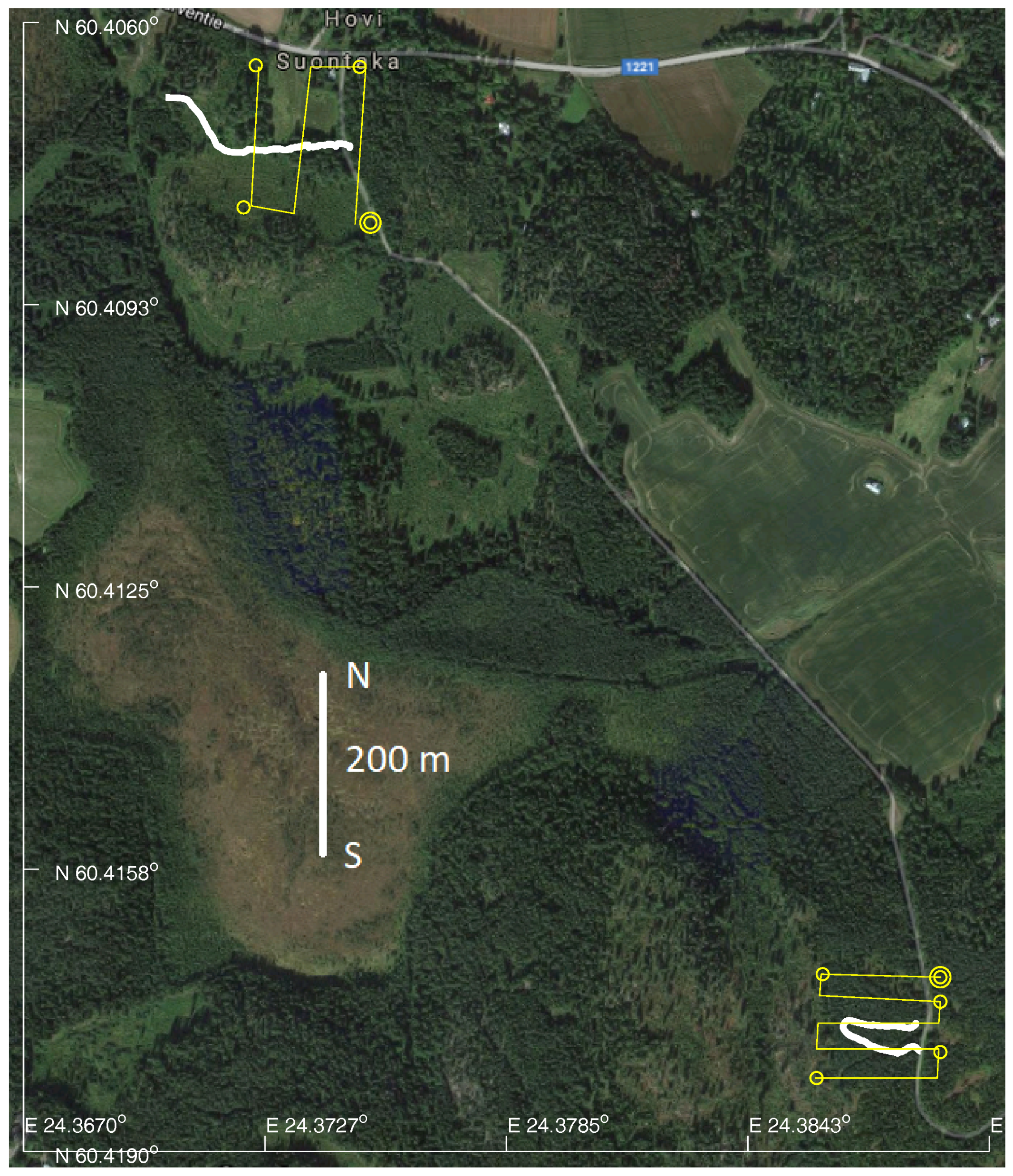
Two sets of four and five ground control points (depicted as circles in Figure 2) were positioned to minimize terrain surface height error and to allow reconstruction of the unified point cloud from aerial images. GPS coordinates of the control points were recorded with a setting of a 5-cm std.position error target with the RTK GeoMax Zenith25 PRO Series. The above mentioned error target can be reached almost immediately in open fields, but the forest canopy imposes difficulties; sometimes, a prolonged period of waiting time was required for a reliable measurement. All measurements were accomplished within a period of 30 min of cumulated field time per site, however.

2.3. Methodology

An overview of the methodology is given here. The subsequent Section 2.5, Section 2.6, Section 2.7 and Section 2.8 go through different stages in detail, while introducing various parameters. Section 2.9 summarizes these parameters.

The TIN models for both the canopy height and the ground model are developed first. The canopy height model is used to improve the quality of the ground model at the fragmented boundaries. The ground model visualization is used for comparing with the manually-measured rut depths. A height convolution iteration is performed at this phase to form a smooth center line. The convolution filter uses the information about the assumed wheel distance of the forest vehicle. The final step is about recording the rut depth profiles.

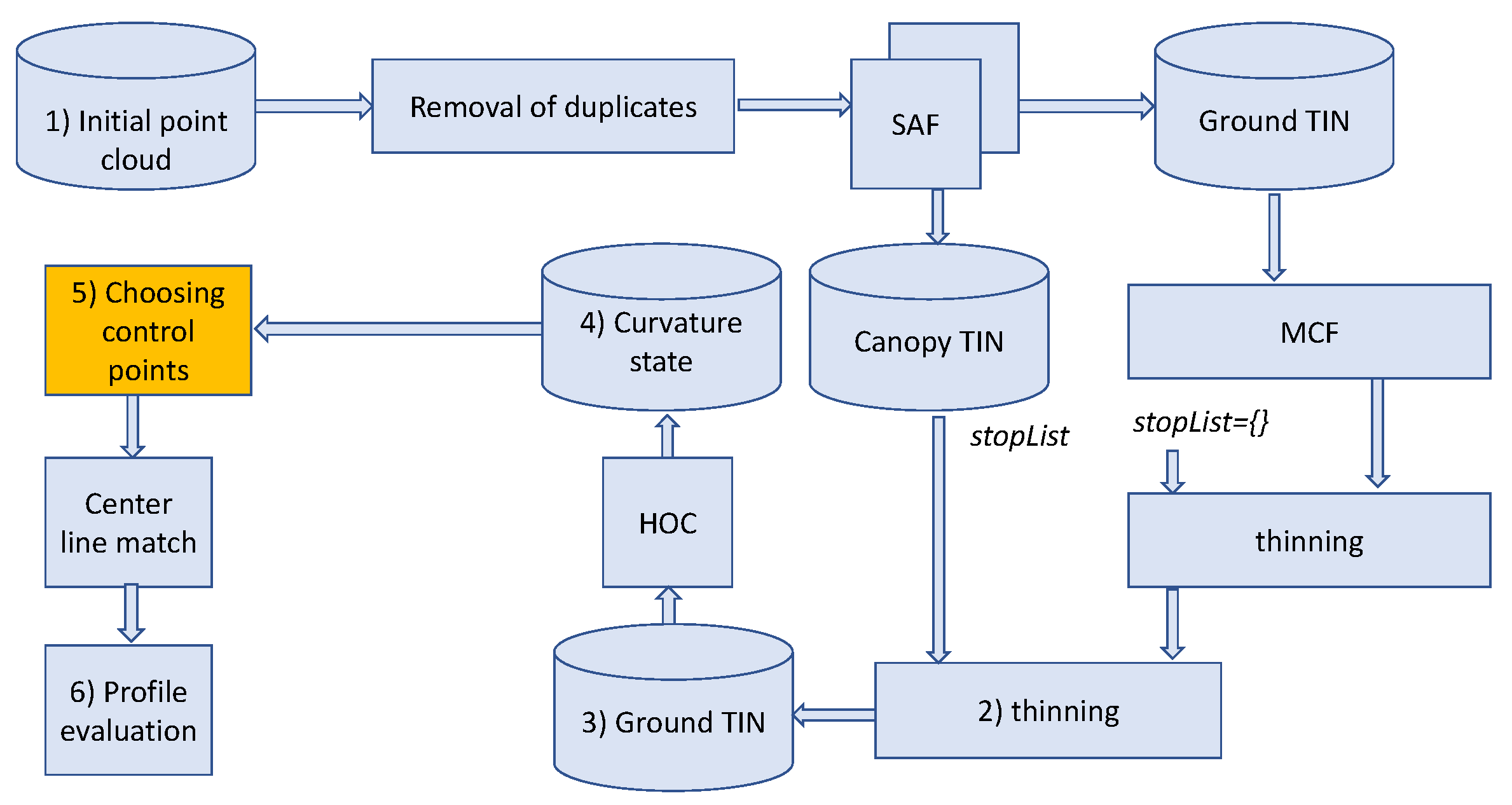
The essential steps of the workflow are: (1) UAV photogrammetry; (2) canopy elimination, forming and visualizing the (4) curvature state of the (3) ground model; (5) finding the central line of the trail and (6) forming the profile model of the ruts; see Figure 3. Many processing steps used have several alternatives, and a rather intense search for various techniques has already been done in the preliminary phase of this study.

Several parameters were used to produce the point cloud, the ground model TIN and the final rut depth profiles. A summary of the parameters can be found in Section 2.9, where all the numerical values are stated.

2.4. Step 0: Point Cloud Generation

The photos taken were processed with AgiSoft PhotoScan Professional software into 3D high-resolution point-clouds. The software applies a structure-from-motion (SFM) process that matches feature-based images and estimates from those the camera pose and intrinsic parameters and retrieves full 3D scene reconstruction [27], which is geo-referenced by ground control points [28]. The geo-reference markers were identified manually in the set of images in which they appeared, and the AgiSoft software performed the necessary geo-referencing using the images, the UAV GNSS/ISS records and the geo-marker pixel and positioning information as the input. Point clouds were re-projected to the ETRS-TM35FIN projection.

2.5. Steps 1, 2: Point Cloud Preprocessing

Proper preprocessing proved to be essential for detecting the rut profiles accurately. Eliminating the direct and secondary effects of the proximity of the canopy was important. Canopy narrows the stripe of the exposed ground and causes a curvature signal. The vegetation and the harvesting residue cause noise and force one to filter and smoothen the TIN in a controlled way.

Two point clouds of Figure 2 and Table 1 have initially an average distance of 6 cm to the horizontally nearest natural neighbor; see Figure 4.

Natural neighbors (NN) are defined by the well-known 2D Delaunay triangulation [29], and those are needed when the ground TIN model is created. The rut detection requires a detailed control over the TIN model production, so we do not use the standard methods available from the GIS and point cloud software. Instead, we apply SAF [25], which utilizes the solid angle ${\omega }_p$ of the “ground cone” associated with each point p. Filtering is based on having all accepted points within the limits ${\omega }_1\le {\omega }_p\le {\omega }_2$ in the resulting TIN.

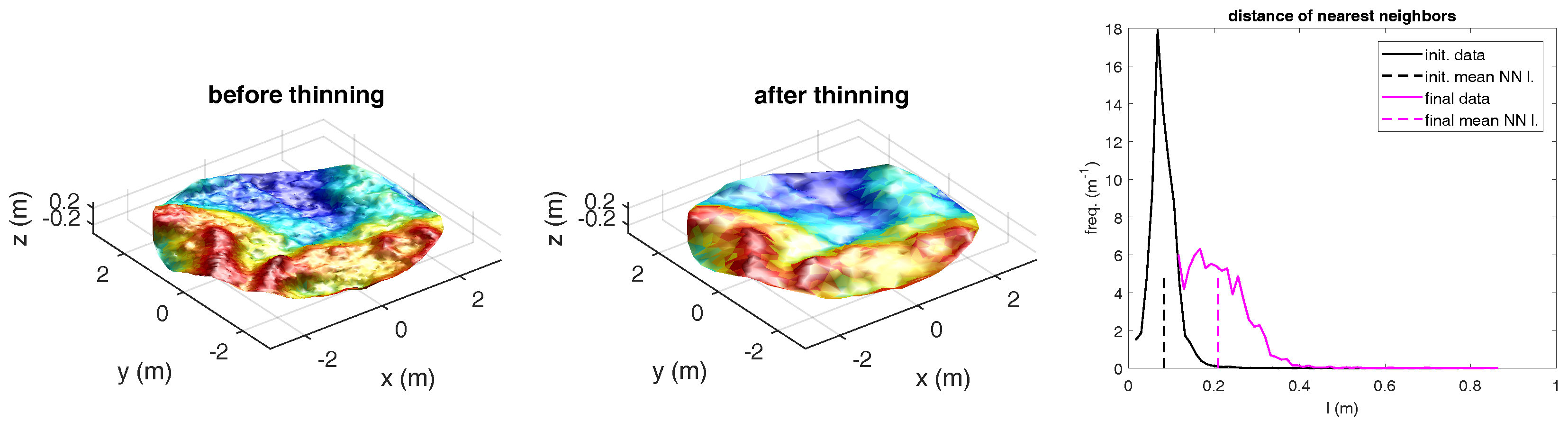
An important descriptor of the point cloud before and after the thinning is the distribution of the triangle edge lengths of the Delaunay triangularization [30]. See Figure 4, left, where two distance distributions (before and after thinning) are depicted.

The preprocessing of the point cloud data consists of a sequence of operations to make the rut depth extraction computations feasible. The operations are listed below:

(a)

Eliminating point pairs with horizontal distance less than $5\mathrm{mm}$. This makes the further processing code simpler. The point above/below gets removed when computing the ground/canopy model, respectively. The minimum distance was decided by the 0.5% data loss criterion. See Figure 4. This process can be done in linear $O(|P|)$ time, where $\left|P\right|$ is the size of the point cloud.

(b)

Building the ground TIN model by applying SAF two times in order to have a structured reduction of the canopy noise at the narrow stripes at the further steps. The first SAF run builds (a) the canopy TIN (green in the middle detail of Figure 5). The model is based on controlled triangularization unlike usual canopy models based on local windows; see e.g., [31]. The second run builds (b) the ground TIN. The spatial angle limit parameters used can be found in Section 2.9. Two models built are used in Steps (c) and (d).

(c)

The mean curvature flow (MCF) [26] was applied to the ground TIN model to smoothen it. The MCF procedure contains one method parameter $\lambda \in \left[0,1\right]$, which controls the aggressiveness of the smoothing effect. MCF is a TIN smoothing method, which resembles the mean filtering of the raster data. It has a typical trade-off between smoothing the noise and possibly deteriorating a useful signal.

(d)

Thinning of the point cloud. Thinning is dictated by the mean natural neighbor distance $\overline{l}$ (see Figure 4), which increases during the process from the preliminary average $\overline{l}=0.07\mathrm{m}$ to the target value $l_b=0.20\mathrm{m}$ in the red zone of Figure 5. The limit value still enables a rather good imprint of the rut shape on the resulting surface triangularization. The green canopy area was subjected to thinning to $l_c=5.0\mathrm{m}$. This was to eliminate the noise at the border areas of the ground model. Parameters $l_b$ and $l_c$ were deemed the most suitable for the further process. See the listing of the actual Algorithm 1.

Figure 6 shows some large TIN triangles produced by the thinning step (d). The large triangles do not contribute to the curvature analysis, since they are eliminated by a triangle size limit $l_{max}=1.2\mathrm{m}$. This is to make it possible to analyze the trails with a very fragmented boundary and the canopy front.

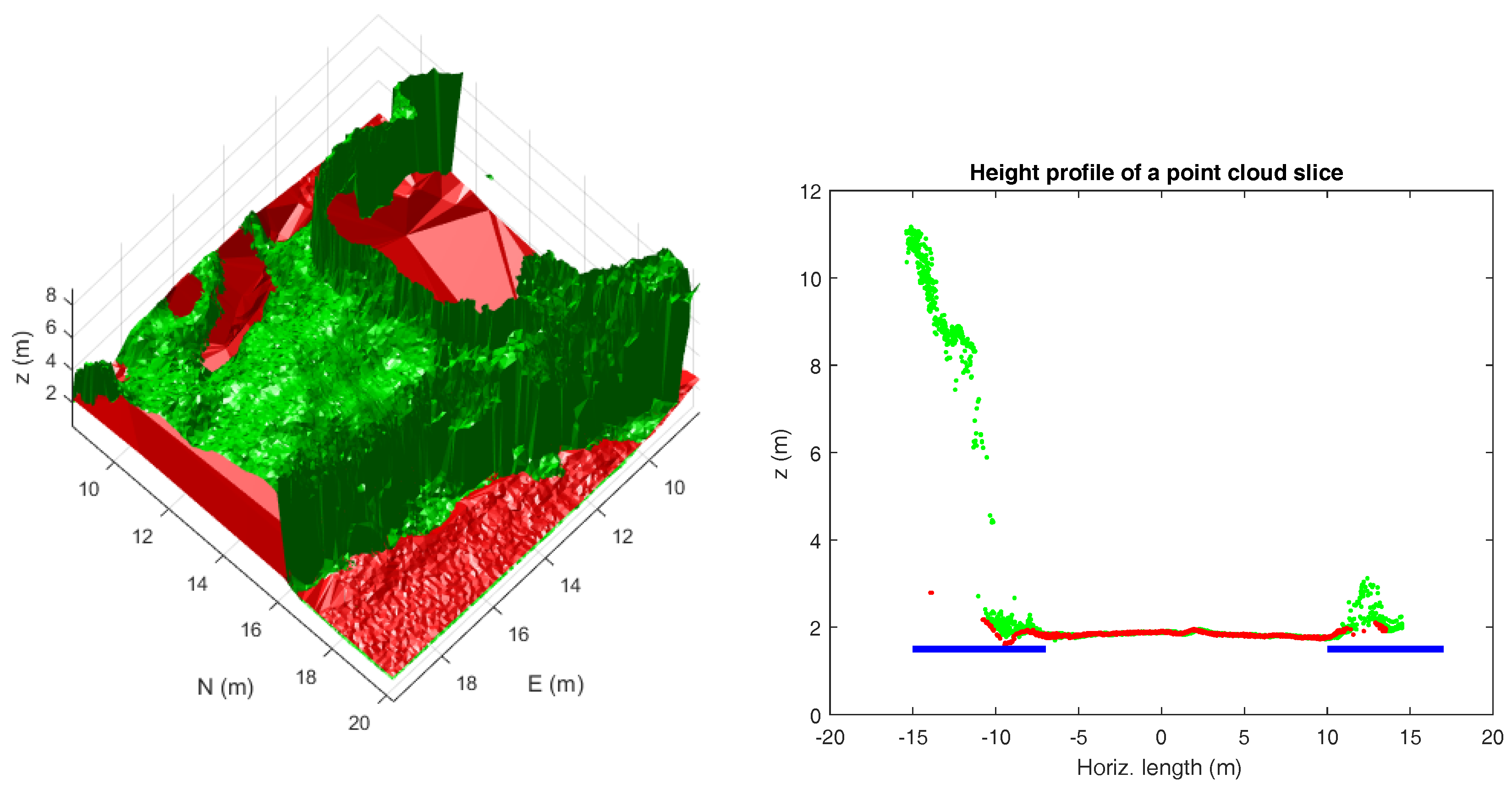
There is the intermediate zone called the canopy front (see the blue horizontal bar at the right side of Figure 5), which is being defined by the height difference of two TIN models. Taking the height difference of two TIN models with independent triangularization is a standard GIS procedure with some subtle practical considerations and speed-ups, which have not been documented here. The end result consists of a mixture of red and blue zones with the canopy part (green) practically disappearing; see Figure 5. The sparse areas have very large triangles (see Figure 6), but the height differences at the canopy front are moderate, i.e., the artificial curvature spike visible in the right detail of Figure 5 becomes partially eliminated. The advantage is that the canopy removal can be achieved without referencing any DEM model.

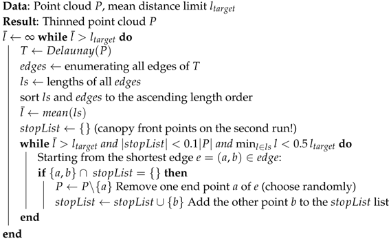
Since the thinning is a non-trivial procedure, it is outlined here. The algorithm runs initially as presented, and the stopList is a list of points already removed. Initially, it is set to be empty; but when the target length $l_b$ has been reached, a new target value $l_c$ will be set, and a second run ensues with the $stopList$ being initialized by a set of the points at the canopy front (a zone indicated by blue bars in Figure 4). This makes it possible to thin the canopy front more heavily. The canopy front is the set of connected ground model triangles with any canopy point above each of the triangles:

Algorithm 1: Thinning the point iteratively making the mean neighborhood distance reach the target value. $l_{target}$ is increased incrementally during the process. Note: The algorithm is applied twice: first, as it is presented, and the second time with the stopList being initiated with the canopy front.

A Delaunay triangulation package providing a batch input, and a dynamical delete is recommended for the algorithm. If no suitable algorithm is available, we recommend space partitioning and slight modification of the algorithm (available from the authors), which thins the TIN as much as is possible until a new TIN is produced in one batch run.

2.6. Steps 3, 4: Trail Detection

Trail detection has two steps: (a) extracting the rotation-invariant curvature state and visualizing the TIN; and (b) manual insertion of the trail control points to initialize the numerical trail center line match.

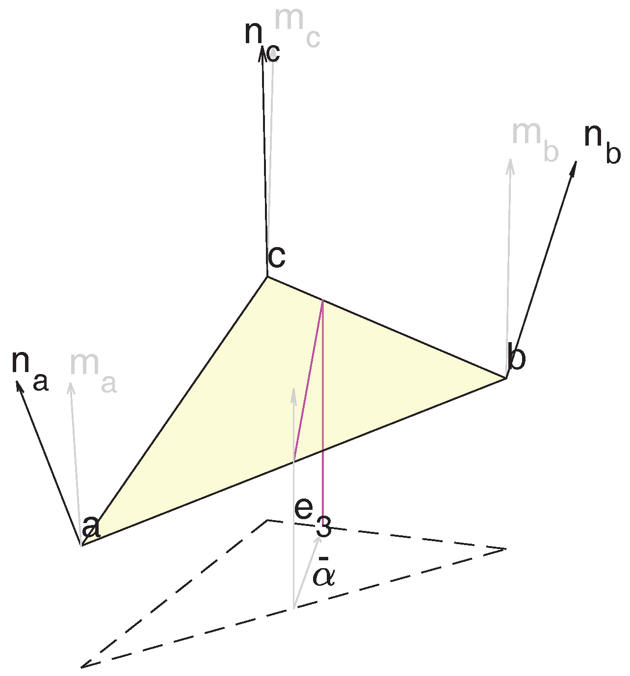
Visualizing the trails: The target area was covered by a grid of circular samples with the grid constant $\delta =3.5$ m and the sample radius $r=2.1$ m. A dominant direction of the curvature was detected from each of the samples using HOC, which is a closely related to the well-known histogram of gradients (HOG) method [32], except that it works with the curvature values. HOC produces histograms of dominant curvatures and the corresponding orientation. The directed curvature is a basic geometric entity along a vertically-oriented plane cutting the TIN surface. The orientation is chosen so that there is a maximum difference between two perpendicularly-oriented curvature histograms; see Figure 7. This arrangement has a rotational invariance.

The directional curvature can be specified for a TIN in a discrete differential geometric (DDG) way. The definition is based on the triangular average of the mean curvature introduced in [33], with the following modification: vertex normals of each triangle are projected to the directional plane before application of the mean curvature equation. The constructed histogram is then weighted by triangle surface areas. The histogram concerns a set of triangles among a sample circle with a radius r with circle centers forming a sample grid with a grid constant $\delta$. The end result seen in Figure 6 was strongly affected by the choice of the sample radius r.

The details of producing the sample histogram $f({\kappa }_{\alpha })$ of the directional curvature ${\kappa }_{\alpha }$ in the orientation $\alpha$ are included in Appendix A. The directional curvatures were produced in $n_{\alpha }=20$ directions. The number of directions was chosen by the exhibited noise level (difference in neighboring directions), which is larger the less directions are chosen and the smaller the samples are. $0\le {\alpha }_i\le \pi ,$ $i=1,\dots ,n_{\alpha }$.

Formally, the curvature state has three components, the orientation ${\alpha }^{\ast }$, the smooth directional curvature histogram $f_1(\kappa )=f({\kappa }_{{\alpha }^{\ast }})$ at the previously-mentioned orientation and the rough directional curvature histogram $f_2(\kappa )=f({\kappa }_{{\alpha }^{\ast }+\pi /2})$, the last two perpendicular to each other. Histograms $f_1$ and $f_2$ are scaled to be distributions observed from Equation (A4). The orientation ${\alpha }^{\ast }$ is chosen by maximizing the directional distribution difference $e(\alpha )$:

$${\alpha }^{\ast }=\arg {\max }_{\alpha }e(\alpha ),$$

(1)

where $e(\alpha )=\frac{1}{2}\int \left|f_1(\kappa )-f_2(\kappa )\right|d\kappa$. Finally, one can define the curvature eccentricity $0\le e\le 1$, extremes associated with isotropic and maximally anisotropic cases, respectively:

$$e=e({\alpha }^{\ast })$$

(2)

The value of the upper limit follows from the fact that both $f_1$ and $f_2$ are distributions. A vectorized representation $\mathbf{x}$ of the curvature state is formed by concatenating $f_1$ and $f_2$:

$$\mathbf{x}=({\{f_1({\kappa }_i)\}}_{i=1,\dots ,n_{\alpha }},{\{f_2({\kappa }_i)\}}_{i=1,\dots ,n_{\alpha }}),$$

(3)

where $i=1,\dots ,n_{\alpha }$ is the bin index of the histograms.

The complete curvature state of each sample window is thus a triplet $(\mathbf{x},e,{\alpha }^{\ast })$, where the feature vector $\mathbf{x}$ identifies the rotationally-invariant local micro-topography, the eccentricity e of Equation (1) characterizes a degree of anisotropy and ${\alpha }^{\ast }$ of Equation (1) holds the orientation. The orientation is indefinite when isotropy is small: $e\approx 0$. 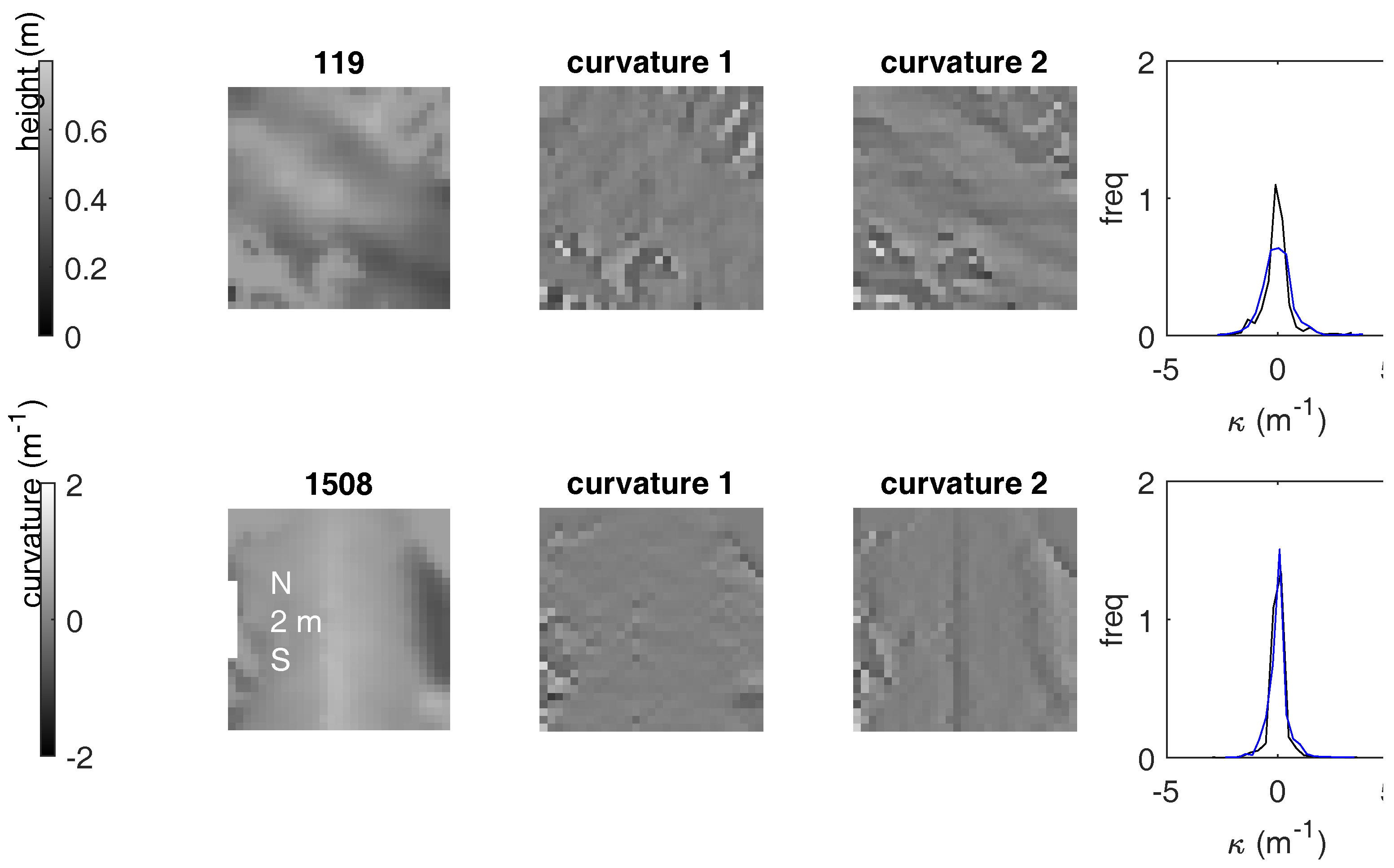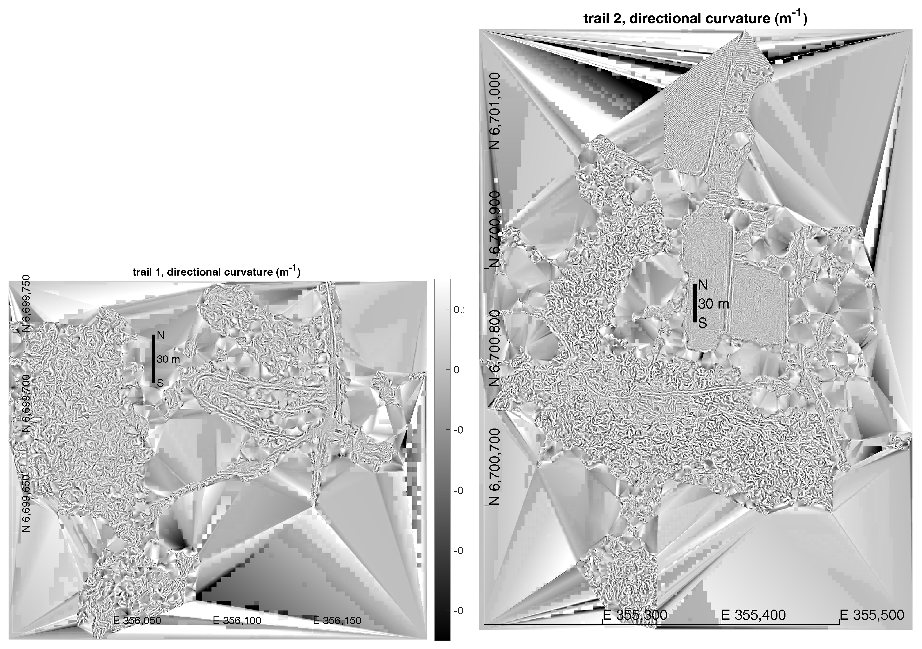Figure 6 shows the directional curvature over the TIN models of Trails 1 and 2. The image has been constructed from the sample grid using the rough directions ${\alpha }^{\ast }+\pi /2$ at each sample grid center.

Figure 7 depicts two spots, one with ruts and one without. The size of the depicted squares is 3.8 m. The boundary inference and noise from the surface vegetation tends to be isotropic, affecting both perpendicular histograms $f_1$ and $f_2$ about the same way, thus not contributing much to the eccentricity e, which is related to the difference of the histograms. A vegetation effect is seen at the upper pair of the curvature images and one boundary effect (a dark patch in the height image) in the lower row.

2.7. Manual Selection of Trails

It is typical to have the presence of older trails from previous operations, and it seems difficult to direct any automatic detection and analysis to the correct recent trails. Hence, manual insertion of proximate trail control points was used. The control points initialize a more accurate numerical trail detection phase described in the next section. The control points are depicted in Figure A4 of Appendix B.

2.8. Steps 4, 5: Profile Evaluation

The first part of the profile evaluation consists of an accurate detection of the trail center line. The second part is about forming the rut depth profile.

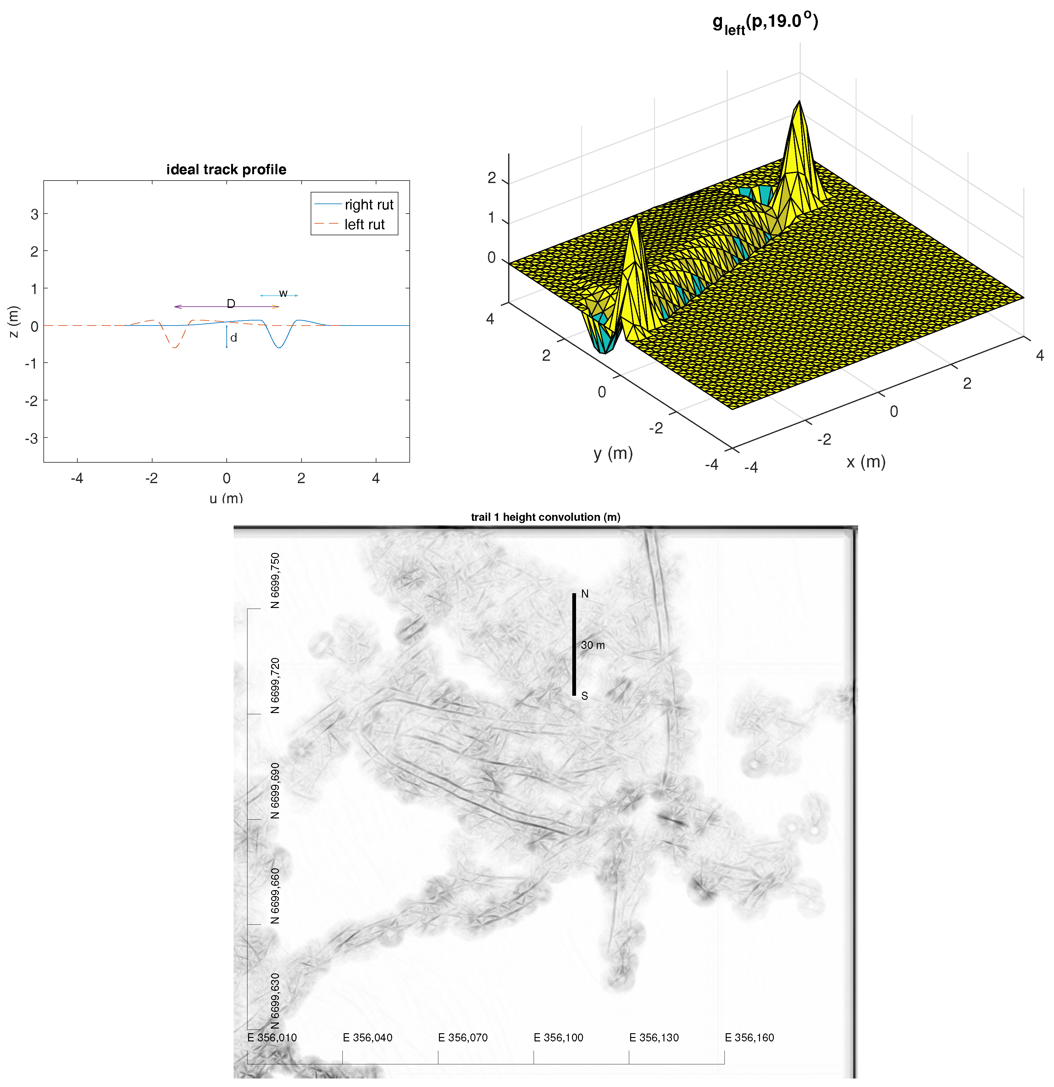
The TIN model was rasterized to a height image of a 0.2-m grid length, which was subjected to a convolution filter depicted in Figure 8 using 20 different orientations. The filter was specifically designed to match the trail created by a typical forest forwarder. The convolution computation in each direction $\alpha$ is fast, and thus, it was performed for the whole area at once. The actual formulation is somewhat involved, since the convolution of ruts is performed by two separate runs and then matched (by an ordinary raster multiplication) from the resulting two images using the rut separation D (the axial length of the forest machine). Convolution in two parts seems to produce a better signal than one single convolution consisting of the left and right ruts. The latter creates three responses, the extra ones with one half of the magnitude of the middle one.

Given the normal 2D convolution operator ⋆, the convolution signal c is:

$$c(p,\alpha )=[z(p)\star g_{left}(p,\alpha )][z(p)\star g_{right}(p,\alpha )],$$

(4)

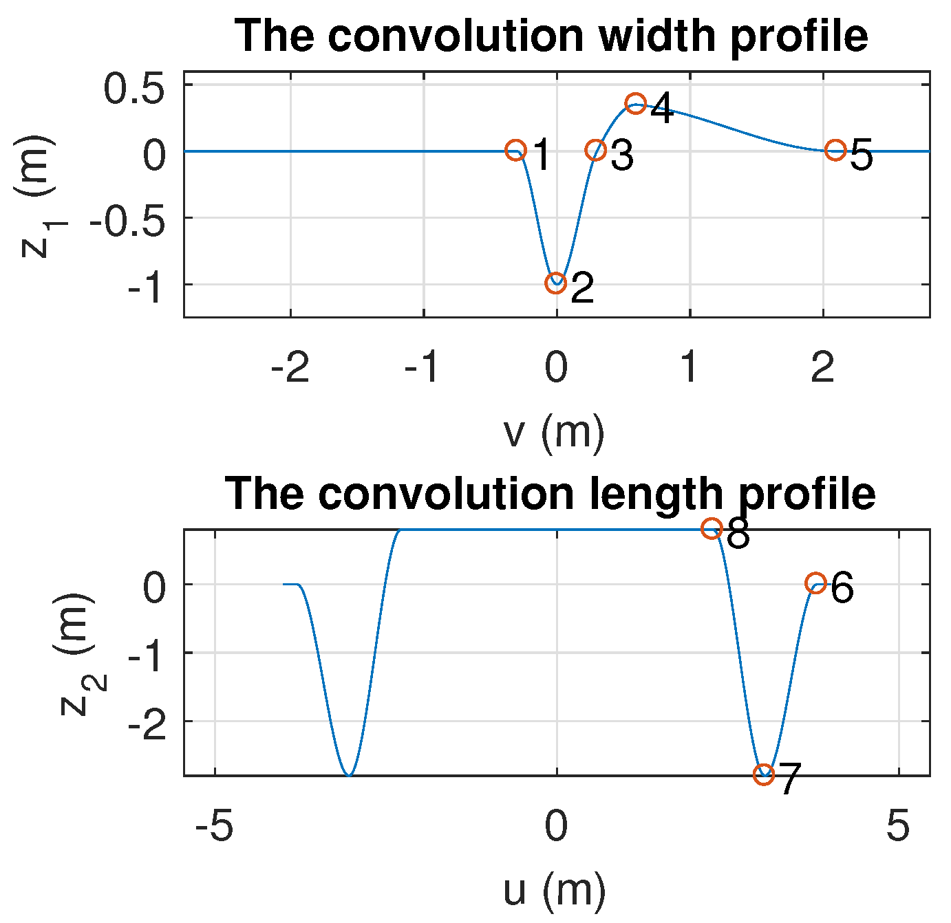
where $z(p)$ is the rasterized TIN height at location p. The ideal trail profile as a combination of filter functions $g_{left}(.)$ and $g_{right}(.)$ of Equation (A5) with the local trail orientation $\alpha$ has been depicted as a projection along the trail in Figure 8 (top left). The top right detail is the convolution filter function $g_{left}$ oriented in this depicted case in a direction $\alpha ={135}^{\circ }$. See the rut profile convolution parameters $D,w,d$ (rut separation, rut width and depth, respectively) used for this particular case in Figure 8 and their values in Section 2.9. The profile convolution is one ingredient to be maximized along the smooth trail center line. The trail line ‘finds’ the response of two ruts depicted by the black end of the grey spectrum in Figure 8 (below). The multiplication arrangement of Equation (4) reduces extra stripes in the image, and the trail pattern triggers only once. Areas without a good signal are spanned by a strong continuity restriction and control points inserted manually. See the further details in Appendix B.1.

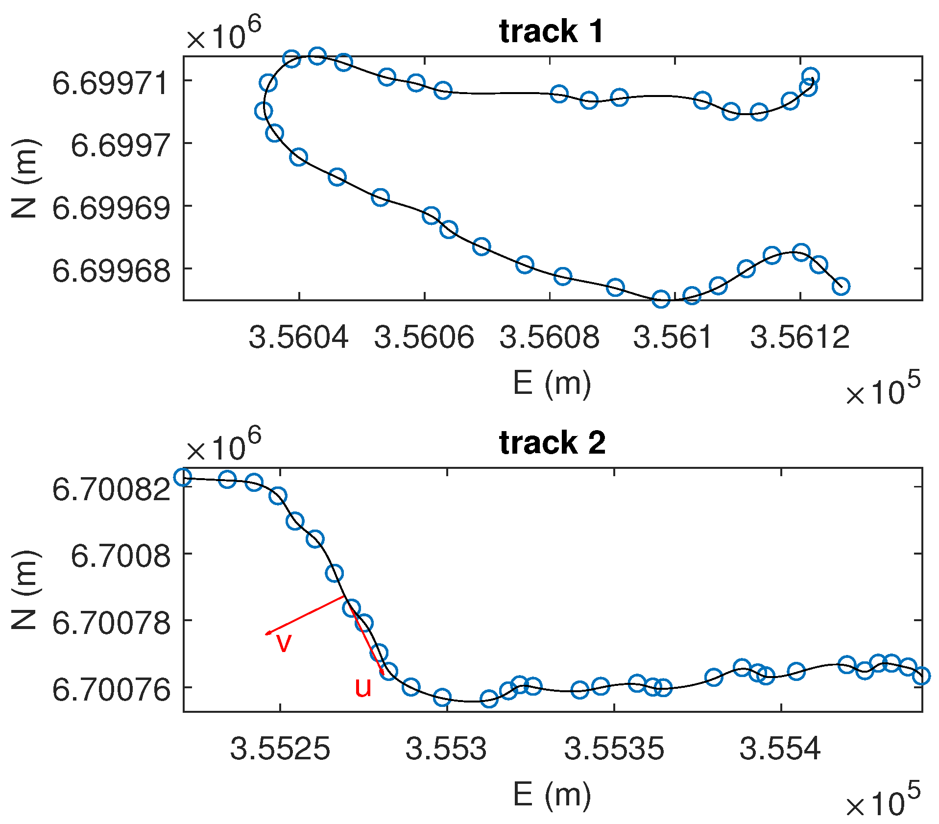
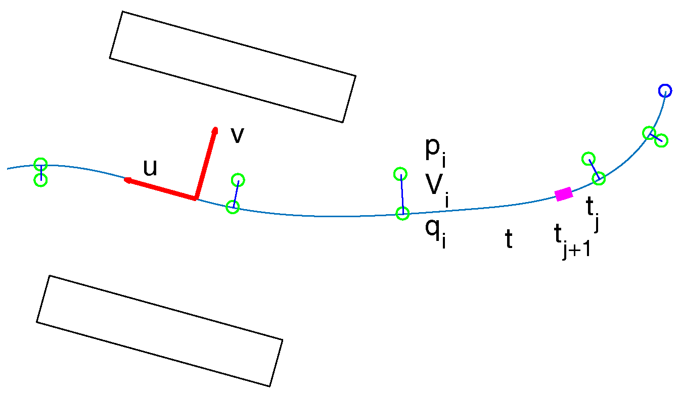
The manual points of Figure A4 outlining the initial trail were used to match a Cornu spline [34] with linear curvature change over the spline length. This spline allows the addition and removal of spline segments without altering the spline shape. The spline was then adjusted by maximizing the convolution match along the trail. The classic nonlinear regularization is based on the curvature squared integrated over the spline length (akin to the nonlinear elastic deformation energy of a thin beam).

A further adjustment was performed using the trail coordinate system with trail relative length t along the spline and the distance v from the spline as the new coordinates. The adjustment involved local shifts along the v axis to track the rut trajectory exactly. Section 3 presents the detected rut depths along the rut length and the average rut cross-profile. The algorithmic details are presented in Appendix B.

2.9. Parameterization

Table 2. The 25 parameters, their values and a short explanation.

Phase	Param. and Value	Explanation
thinning	$l_{target}=0.2\mathrm{m}$	thinning limit
thinning	$0.1\left|P\right|$	stopList size limit
thinning	$0.5l_{target}$	triangle edge length limit
vectorization	$r=2.1$ m	sample radius
	$\delta =3.5$ m	sample grid interval
SAF canopy	${\omega }_1=\pi$	pike limit
	${\omega }_2=3\pi$	hole limit
SAF ground	${\omega }_1=4.4$
	${\omega }_2=8.1$
MCF	$\lambda =0.7$	smoothing degree
thinning	$l_b=0.2$ m	NN length at ground
	$l_c=5.0$ m	NN length at canopy front
trail detection	$n_{\alpha }=20$	number of curvature directions
profile evaluation	$D=2.8$ m	rut distance
	$w=1.2$ m	rut width
	$d=0.6$ m	rut depth (no actual effect)
	$r_{rut}=3.8$ m	convolution sample length
	medium
	$\Delta L=0.2$ m	rut profile sampling interval
	7 free shape params.	see Table A1
convolution fit	${\lambda }_1=0.7{\mathrm{m}}^2$	regularization weight
	$\Delta l=0.6\mathrm{m}$	convolution sampling frequency

lists all the parameters used. Actual cross-validation verification of the values shown has not been included. Some justifications of the values have been given in the text.

3. Results

The initial filtering by SAF, MCF and thinning described in Algorithm 1 produces the point cloud, which is the basis for the further curvature analysis. An ideal regular triangular lattice with a 20-cm side length (the set value used) has the horizontal point cloud density ${\rho }_{ideal}=14.4{\mathrm{m}}^{-2}$. The resulting ground model has a very high quality with density very close to the ideal one; see

Table 3. The point cloud properties. Horizontal densities $\rho$ are in m${}^{-2}$. The abbreviations TP, TN, FP and FN correspond to true and false positives and negatives given as percentages.

Trail	Initial $\mathit{\rho }$	$\mathit{\rho }$ TIN	$\mathit{\rho }$ after Thinning	TP (%)	TN (%)	FP (%)	FN (%)
1	190	120	16	19	51	26	4
2	180	117	15	38	24	24	14

. The given values are for the canopy openings, since the earlier processing reduces the density of the canopy area to a much lower value ($\rho <1{\mathrm{m}}^{-2}$; see Figure 6).

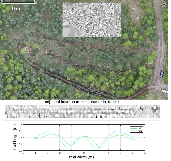
TIN models were generated from the photogrammetric point cloud at two target areas (Trails 1 and 2), in Figure 1; curvature vectors were recorded from a regular grid of sample locations (see Table 2) using the histograms of dominant directions, and the rut profiles were analyzed from the TIN model. Some results like the canopy and ground TIN models have been made available for an undetermined time period; see the Supplementary Materials on p. 18.

In Finland, the Government Decree on Sustainable Management and Use of Forests (1308/2013) based on the Forest Act (1093/1996) and related field control instructions by the Finnish Forest Centre, Helsinki, Finland (2013) regulate that rut depths of 10 cm (mineral soils) and 20 cm (peatlands) are classified as damage and can be detrimental to the forest growth. Table 3 gives a summary of detecting particularly the 20-cm depth: P (positive) stands for a depth more than 20 cm, N (negative) for a depth less than 20 cm and, e.g., TP and FN stand for the ratio of the sum of correctly-detected deep rut sections and deep sections not recognized, correspondingly. The overall accuracy (sum of TP and TN weighted by the trail lengths) is 65%. The performance is adequate for the purposes of the quality assurance of forest operations considering the amount of data that can be possibly collected compared to traditional methods.

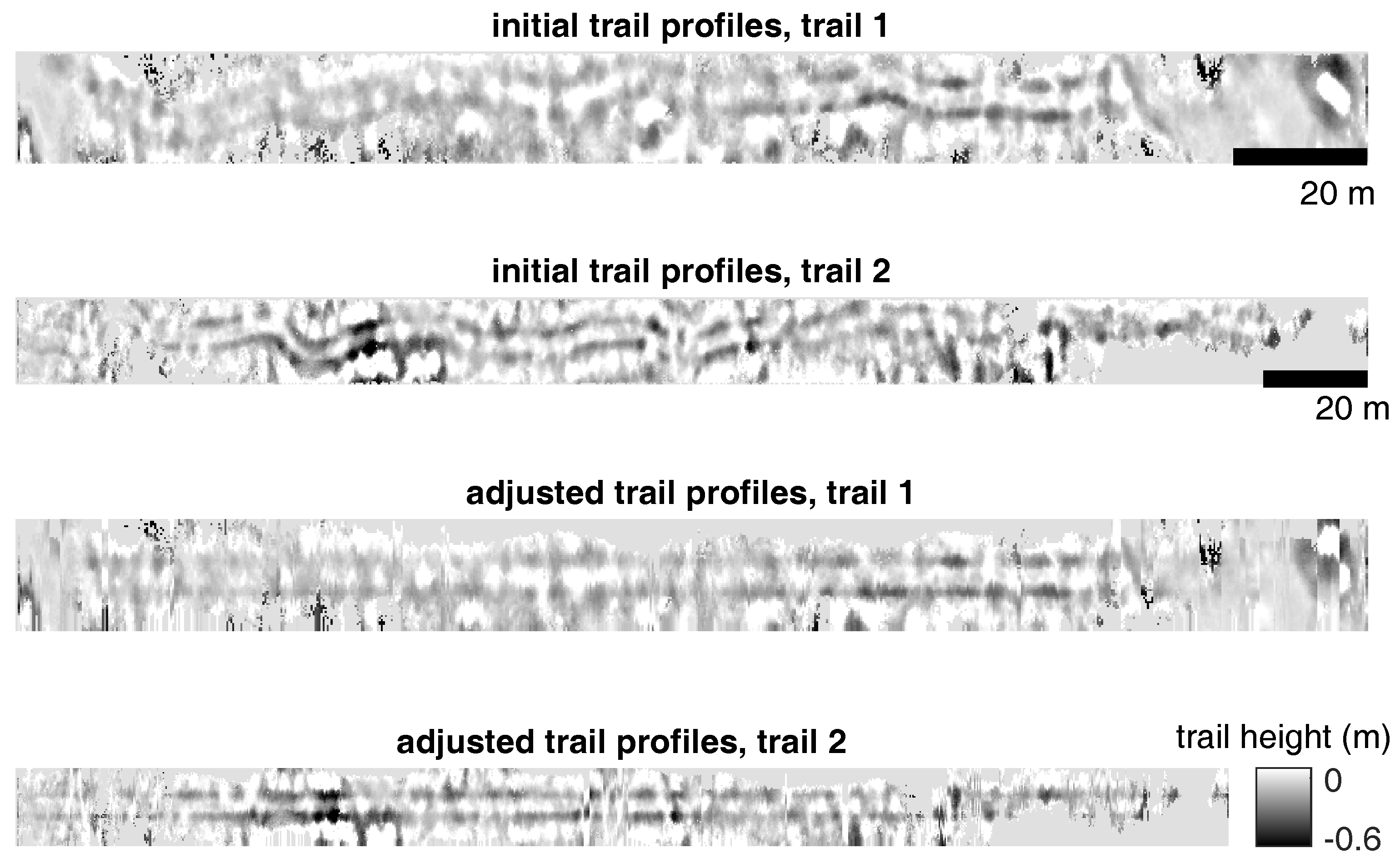
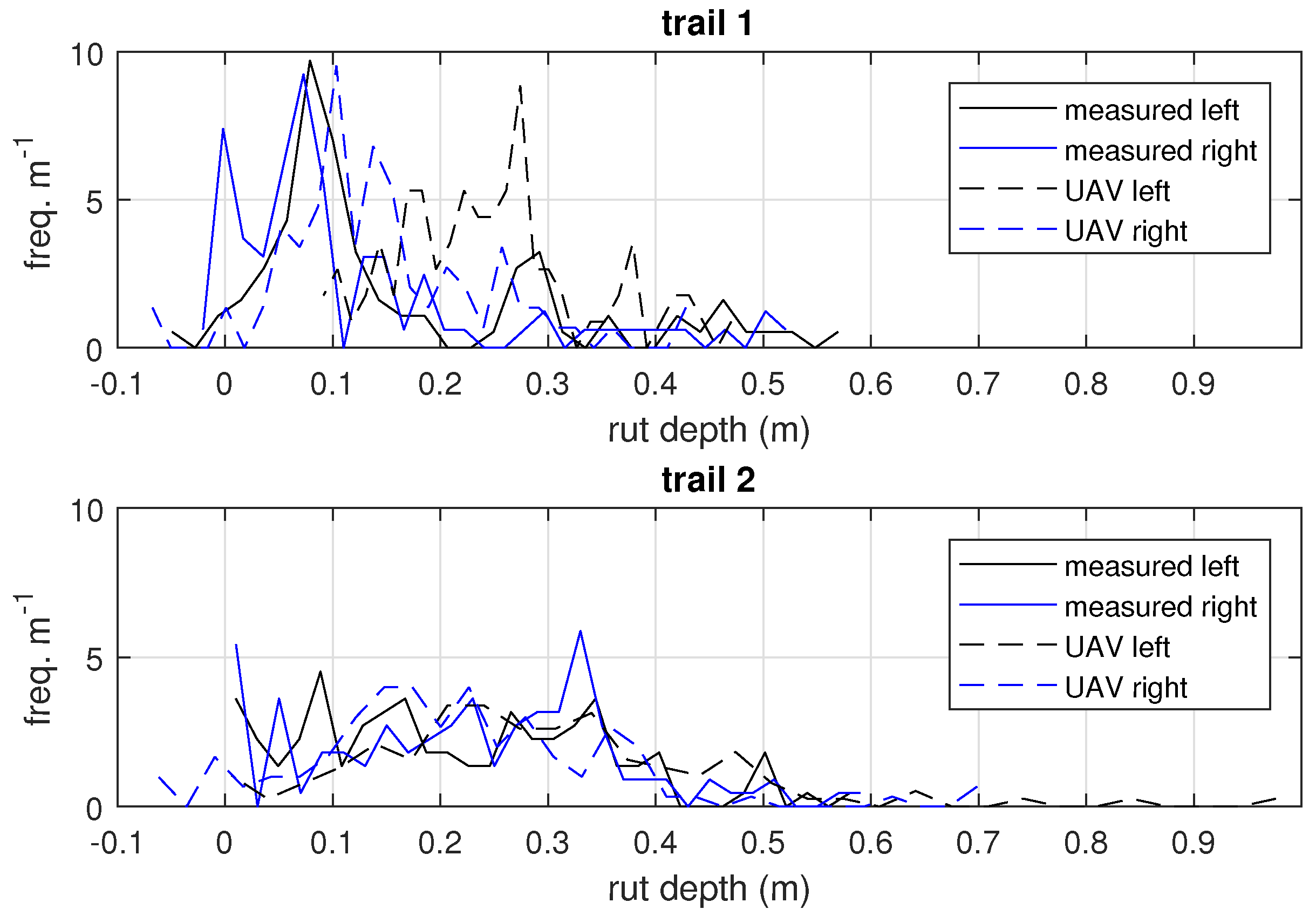
After manual identification of the control points on trails, the center lines of trails were adjusted automatically by the convolution penalty, and the rut depth profiles were formed. Figure 9 shows the depth distributions along both trails on both manual and UAV measurements. Really deep depressions are rather rare, and they tend to become detected better. The UAV measurement detected much more of the depth 0.2–0.3 m range than the manual measurement on Trail 1. Trail 2 has a good correspondence between the manual and UAV measurements. The trail depth classification is in general worse in the presence of nearby trees.

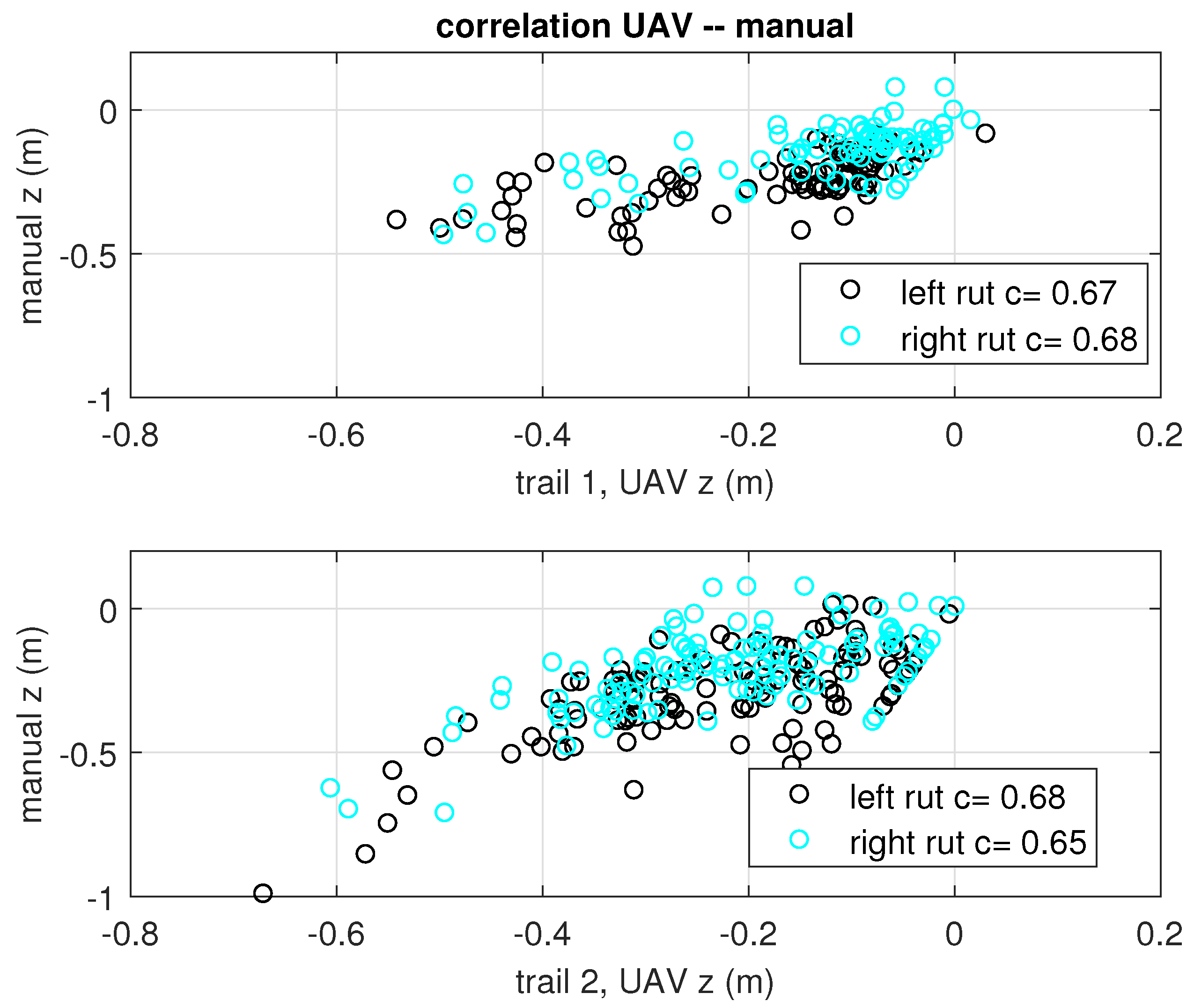
Pearson’s r correlation was taken between UAV and manual rut depth values at each manual measurement point; see Figure 10. The correlation $r=0.67$ relates to the following inaccuracies: horizontal placement error of the point cloud and the reference level estimation in the manual measurement.

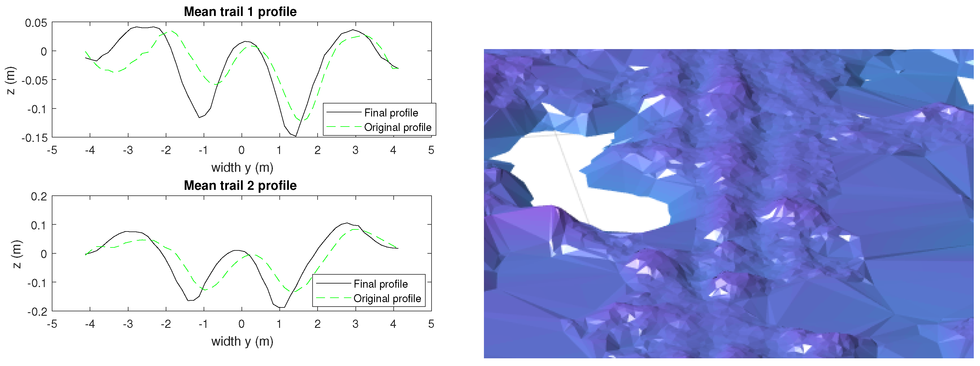
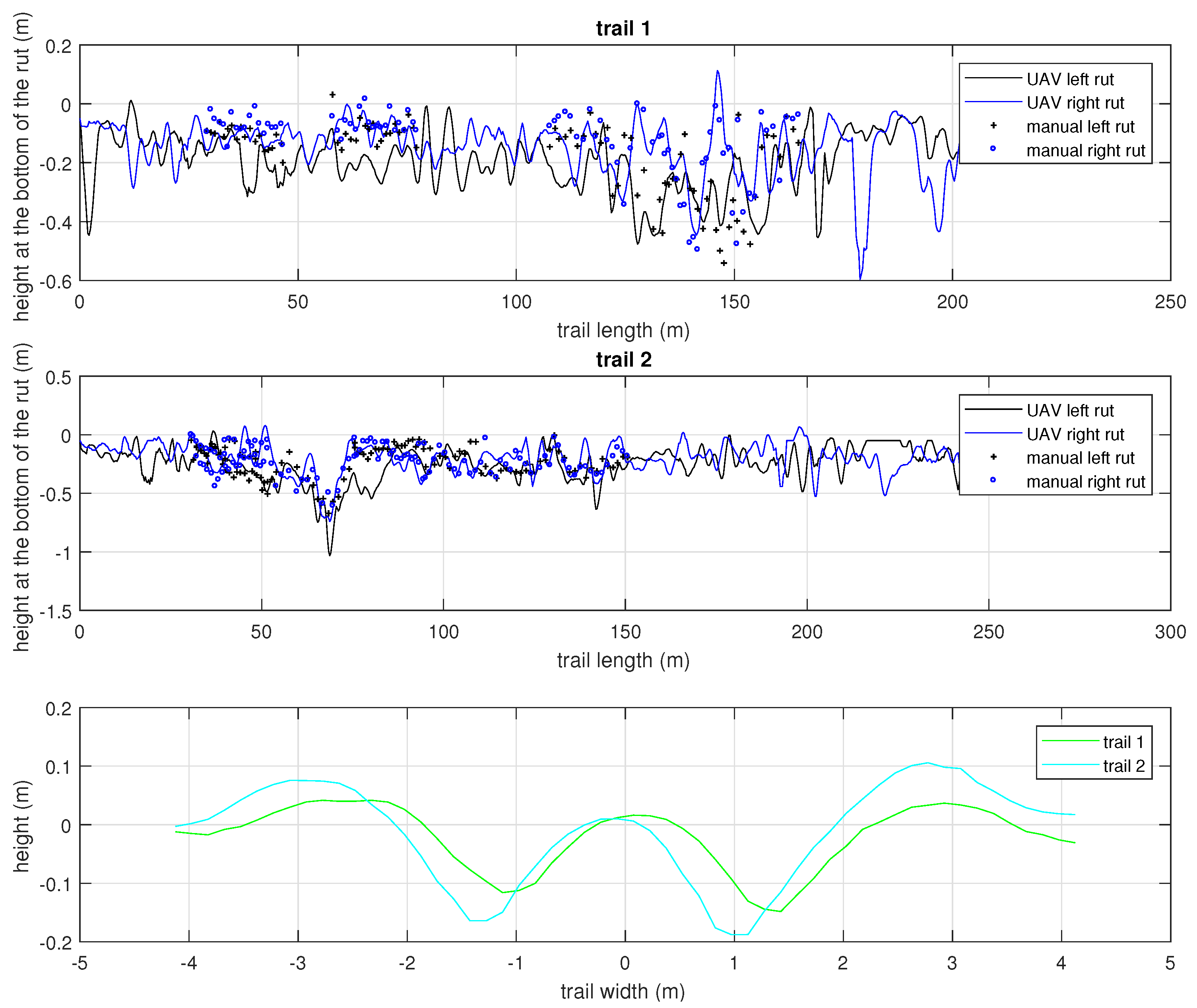
Figure 11 demonstrates how large differences can occur between two ruts. Some rocks and roots (each correctly identified) force the rut to have positive (above the reference level) heights. Multiple passes deteriorate the shape of the rut, but the average shape is relatively constant over large distances and similar terrain. The averaged trail profile shows typical displacement of the soil. The effect of slopes has been removed, but a long sideways slope causes one of the ruts to become deeper (the right rut of Trail 2 in Figure 11).

4. Discussion

The experiments of registering the rut depths by UAV photogrammetric point cloud are a part of a larger research project, e.g., [22], on traversability prediction. Thus, the site was emulating a typical forestry operation dictating payload amounts, machinery used and number of passes.

Figure 9 shows how the UAV measurement detected much more of the depth 0.1–0.3 m range than the manual measurement on Trail 1. This can be explained by difficulties in defining the control surface level in a compatible fashion by both methods (manual and UAV) on certain terrain conditions. The manual reference level tends to be assessed by humans from the proximity of the rut, whereas the UAV method fits the reference height origin (0-m level of the trail cross-profiles of Figure 11). Neither reference level is imperfect per se, but it seems that the calibration measurements should be done within an artificial environment with absolute measures, or with a ground-based LiDAR scanner, for example, which provides the chance to match the reference height of two point clouds reliably.

The point cloud need not to be geo-referenced nor matched to the DEM. This allows a UAV flight path that is reduced to cover only the trails with only a necessary amount of overlapping to enable the photogrammetric 3D point cloud generation. The RGB information would add to trail registration performance, but requires more research and more varied test materials with different weather, soil, terrain and light conditions.

The following is a short presentation of the observations of the experiments with alternative techniques (not including the proposed methodology presented in the Section 2.3):

Point cloud preprocessing: We extracted the curvature state of the ground model in order to expose the trails from the data. Subtracting the DEM height from the point cloud provides an easy way to eliminate the canopy points, but the resulting algorithm would not cope well in countries and sites with no ubiquitous DEM model. Furthermore, it requires careful planning and placement of the geo-referencing markers to reach the, e.g., $\pm 1\mathrm{m}/100\mathrm{m}$ height accuracy required with the two sites used in this study.

Ground height model: We produced TIN using a solid angle filtering [25] method. The local linear fit of [35] is a computation-intensive method, which does not adapt well to the noise from the canopy wall around the trail. Various heuristics such as taking the local mean of the lowest point cloud points after a space division to small compartments (approximately 20–30 cm) forces a repetitive inefficient computation and is not suitable for parameter optimization. Traditional local quadratics methods applied to the 3 × 3 raster window used to derive the DEM models [36] in geographic information systems (GIS), when scaled to the UAV point cloud density (≈80 m${}^{-2}$ at the surface), smoothed the rut contour too much and did not provide adequate control for proper signal processing optimizations.

Vectorization: Vectorization is needed to detect a possible rut present locally and to assess the possible orientation of it. We used a novel histogram of curvatures (HOC) approach. There are several possibilities uncharted yet, including image difference methods based on entropy and information measures. Furthermore, all possible sampling radii and sample grid densities have not been fully covered yet. No adequate combination of machine learning methods, features and cloud preprocessing has been found yet to detect the ruts automatically with a reliable performance.

Neighborhood voting: It is possible to improve the track analysis by smoothing and strengthening the orientation information. There are several promising neighborhood voting methods, which need to be adapted only a little to this problem, but the basic signal from the vectorization phase has to be improved first.

Finding the trail center line: Trails can have a complicated structure, the proper handling of which has not been added yet. Early experiments with principal graphs using the software of [37] seem to be capable of handling loops, branches and junctions. It seems to be mathematically possible to utilize the local orientation information of [37], but at the moment, the noise level of the orientation is too high. The noise signal of the small trees, which do not completely get eliminated by solid angle filtering (SAF) [25], is particularly problematic. Multiple classification to ruts/young trees/open ground/canopy could be a solution.

Several experiments were made to automate the trail detection. Two major difficulties are: (1) finding methods generic enough to cope with most of the environmental conditions, especially with trails partially covered by the canopy; and (2) speeding up the initial processing steps. At the moment, the initial point cloud generation by photogrammetry is too slow for any online approach that would allow the automated flight control and autonomous flight path planning. At the moment, one is limited to a pre-defined flight pattern and batch processing after the field campaign.

5. Conclusions

We aim at a streamlined and economical workflow, which could be used after the harvesting operations both for collecting extensive ground truth data for trafficability prediction models and as a generic post-harvest quality assessment tool. A novel method of cumulating histograms of directed curvatures (HOC) is proposed, which reduces the computational burden of curvature analysis of the TIN samples. We demonstrate the procedure comparing the results with the field data collected from a test site. The procedure contributes towards automated trail detection and rut depth evaluation.

The proposed procedure can classify rut depths into two categories (insignificant depression/harmful rut depth) with practical precision using approximately 10 UAV images per 100 m of trail length. It is relatively inexpensive, since it is independent of the following conditions:

• before-after type of data collection
• GPS data of harvesting routes
• geo-referencing for utilizing the digital elevation maps (DEM)

The UAV requires the visual contact of the operator. This is more a legislation restriction, which could be removed in the future.

A proper point cloud pre-processing seems to be essential when using UAV point clouds for rut depth analysis and similar micro-topography tasks. The profile analysis based on manual control points is already ready for a practical tool implementation, while the pre-processing requires some practical improvements to be used with cross-validation or with neural network methods. Especially the segmentation into several classes, e.g., young trees, dense undergrowth and ruts, could be useful. Furthermore, a combination of the slope and curvature histograms and other pattern recognition methods has to be tested in the future.

The flight height of 100 m seems adequate with the equipment used. Experiments have to be performed with atypical flight plans with no geo-referencing and focusing the flight path on the trails more closely. These experiments will require direct structure-from-motion methods that are based on numerically-estimated camera positions, and the resulting point cloud has slightly lower spatial accuracy [38].

The 65% accuracy in classifying deep ruts (depth of over 20 cm) is adequate for practical purposes, e.g., as a post-harvest quality assurance. More extensive calibration data have to be produced to evaluate the performance in order to contribute to the on-going research of trafficability prediction. The combination of the canopy height model produced by UAV photogrammetry and the ground TIN produced by a more deeply-penetrating aerial LiDAR scan has to be studied in the future. This combination could contribute to understanding the relation between the rut formation and tree roots.

An efficient pipeline for rut depth field measurements is an essential step in gaining understanding about the interplay between environmental factors described by the public open data and the scale and nature of the variations caused to, e.g., cross-terrain trafficability [22] by the micro-topography. The current size of the test site is not adequate for final assessment of the future rut depth classification performance, but the suggested methodology based on UAV photogrammetry, ground TIN based on the SAF method, directional curvature analysis and using either manual or automatic trail detection seems to have potential.

As [16] states, the reference ground level (namely the ground level before the trail was formed) remains difficult to define by any means, including the best possible ground-based laser scanning and human assessment. The rut depth evaluation has to have some categorical element, addressing mainly two or three rut depth classes.

In the long run, the cloud pre-processing + SAF + MCF + thinning should be implemented either using existing software or a separate application to be developed. There is an on-going effort to streamline this process so that it behaves monotonically under usual cross-validation procedures in order to allow efficient parameter optimization for various machine learning tasks. The HOC procedure (generation of directed curvatures directly from TIN) is a novel generic technique, which will be a part of future attempts at vectorizing the ground models of both LiDAR and UAV photogrammetric origin in order to classify ruts and other useful micro-topographic features automatically at a large scale.

References

1. Cambi, M.; Certini, G.; Neri, F.; Marchi, E. The impact of heavy traffic on forest soils: A review. For. Ecol. Manag. 2015, 338, 124–138. [Google Scholar] [CrossRef]
2. Duncker, P.S.; Raulund-Rasmussen, K.; Gundersen, P.; Katzensteiner, K.; Jong, J.D.; Ravn, H.P.; Smith, M.; Eckmüllner, O.; Spiecker, H. How forest management affects ecosystem services, including timber production and economic return: Synergies and trade-offs. Ecol. Soc. 2012, 17, 50. [Google Scholar] [CrossRef]
3. Owende, P.; Lyons, J.; Haarlaa, R.; Peltola, A.; Spinelli, R.; Molano, J.; Ward, S. Operations Protocol for eco-Efficient Wood Harvesting on Sensitive Sites. Developed by the ECOWOOD Partnership. 2002. Available online: http://www.ucd.ie/foresteng/html/ecowood/op.pdf (accessed on 8 December 2017).
4. Pierzchala, M.; Talbot, B.; Astrup, R. Measuring wheel ruts with close-range photogrammetry. Forestry 2016, 89, 383–391. [Google Scholar] [CrossRef]
5. Quesnel, H.; Curran, M. Shelterwood harvesting in root-disease infected stands—Post-harvest soil disturbance and compaction. For. Ecol. Manag. 2000, 133, 89–113. [Google Scholar] [CrossRef]
6. Sirén, M.; Ala-Ilomäki, J.; Mäkinen, H.; Lamminen, S.; Mikkola, T. Harvesting damage caused by thinning of Norway spruce in unfrozen soil. Int. J. For. Eng. 2013, 24, 60–75. [Google Scholar] [CrossRef]
7. Vega-Nieva, D.J.; Murphy, P.N.; Castonguay, M.; Ogilvie, J.; Arp, P.A. A modular terrain model for daily variations in machine-specific forest soil trafficability. Can. J. Soil Sci. 2009, 89, 93–109. [Google Scholar] [CrossRef]
8. Curzon, M.T.; D’Amato, A.W.; Palik, B.J. Harvest residue removal and soil compaction impact forest productivity and recovery: Potential implications for bioenergy harvests. For. Ecol. Manag. 2014, 329, 99–107. [Google Scholar] [CrossRef]
9. PEFC. Programme for the Endorsement of Forest Certification: PEFC International Standard. 2010. [Google Scholar]
10. FSC. Forest Stewardship Council: FSC International Standard, FSC Principles and Criteria for Forest Stewardship. 2015. [Google Scholar]
11. Centre, F.F. Suomen Metsäkeskuksen Maastotarkastusohje (Field control instructions of Finnish Forest Centre). Technical Report, Finnish Forest Centre, 2016. Available online: http://www.metsakeskus.fi/sites/default/files/smk-maastotarkastuohje.2016.pdf (accessed on 8 December 2017).
12. Eliasson, L.; Wästerlund, I. Effects of slash reinforcement of strip roads on rutting and soil compaction on a moist fine-grained soil. For. Ecol. Manag. 2007, 252, 118–123. [Google Scholar] [CrossRef]
13. Pierzchała, M.; Talbot, B.; Astrup, R. Estimating soil displacement from timber extraction trails in steep terrain: Application of an unmanned aircraft for 3D modelling. Forests 2014, 5, 1212–1223. [Google Scholar] [CrossRef]
14. Uusitalo, J.; Ala-Ilomäki, J. The significance of above-ground biomass, moisture content and mechanical properties of peat layer on the bearing capacity of ditched pine bogs. Silva Fennica 2013, 47, 1–18. [Google Scholar] [CrossRef]
15. Ala-Ilomäki, J. Metsäisten Turvemaiden Kulkukelpoisuus (Trafficability of Forested Peatlands); Technical Report; Nature Resource Center of Finland (LUKE): Helsinki, Finland, 2005. [Google Scholar]
16. Salmivaara, A.; Miettinen, M.; Finér, L.; Launiainen, S.; Korpunen, H.; Tuominen, S.; Heikkonen, J.; Nevalainen, P.; Sirén, M.; Ala-Ilomäki, J.; et al. Wheel rut measurements by forest machine mounted LiDAR sensor. Accuracy and potential for operational applications? Int. J. For. Eng. 2018. submitted. [Google Scholar]
17. Nouwakpo, S.K.; Huang, C.H. A simplified close-range photogrammetric technique for soil erosion assessment. Soil Sci. Soc. Am. J. 2012, 76, 70–84. [Google Scholar] [CrossRef]
18. Haas, J.; Hagge Ellhöft, K.; Schack-Kirchner, H.; Lang, F. Using photogrammetry to assess rutting caused by a forwarder—A comparison of different tires and bogie tracks. Soil Tillage Res. 2016, 163, 14–20. [Google Scholar] [CrossRef]
19. Koreň, M.; Slančik, M.; Suchomel, J.; Dubina, J. Use of terrestrial laser scanning to evaluate the spatial distribution of soil disturbance by skidding operations. iForest Biogeosci. For. 2015, 8, 386–393. [Google Scholar] [CrossRef]
20. Lisein, J.; Pierrot-Deseilligny, M.; Bonnet, S.; Lejeune, P. A Photogrammetric Workflow for the Creation of a Forest Canopy Height Model from Small Unmanned Aerial System Imagery. Forests 2013, 4, 922–944. [Google Scholar] [CrossRef]
21. Waldhauser, C.; Hochreiter, R.; Otepka, J.; Pfeifer, N.; Ghuffar, S.; Korzeniowska, K.; Wagner, G. Automated Classification of Airborne Laser Scanning Point Clouds. Solving Comput. Expens. Eng. Probl. Math. Stat. 2014, 97, 269–292. [Google Scholar]
22. Pohjankukka, J.; Riihimäki, H.; Nevalainen, P.; Pahikkala, T.; Ala-Ilomäki, J.; Hyvönen, E.; Varjo, J.; Heikkonen, J. Predictability of boreal forest soil bearing capacity by machine learning. J. Terramech. 2016, 68, 1–8. [Google Scholar] [CrossRef]
23. Kim, A.M.; Olsen, R.C. Detecting trails in LiDAR point cloud data. In Proceedings of the SPIE, Baltimore, MD, USA, 14 May 2012; Volume 8379. [Google Scholar]
24. Kalbermatten, M.; Ville, D.V.D.; Turberg, P.; Tuia, D.; Joost, S. Multiscale analysis of geomorphological and geological features in high resolution digital elevation models using the wavelet transform. Geomorphology 2012, 138, 352–363. [Google Scholar] [CrossRef]
25. Nevalainen, P.; Middleton, M.; Sutinen, R.; Heikkonen, J.; Pahikkala, T. Detecting Terrain Stoniness From Airborne Laser Scanning Data. Remote Sens. 2016, 8, 720. [Google Scholar] [CrossRef]
26. Desbrun, M.; Meyer, M.; Schröder, P.; Barr, A.H. Implicit Fairing of Irregular Meshes Using Diffusion and Curvature Flow. In Proceedings of the 26th Annual Conference on Computer Graphics and Interactive Techniques, SIGGRAPH ’99, Los Angeles, CA, USA, 8–13 August 1999; ACM Press/Addison-Wesley Publishing Co.: New York, NY, USA, 1999; pp. 317–324. [Google Scholar]
27. Wu, C. Visualsfm: A Visual Structure From Motion System. 2011. Available online: http://ccwu.me/vsfm/ (accessed on 8 December 2017).
28. Agisoft. Agisoft PhotoScan User Manual: Professional Edition, Version 1.1.; Agisoft: St. Petersburg, Russia, 2012. [Google Scholar]
29. De Berg, M.; Cheong, O.; van Kreveld, M.; Overmars, M. Computational Geometry: Algorithms and Applications, 3rd ed.; Springer: Santa Clara, CA, USA, 2008. [Google Scholar]
30. Devillers, O. On Deletion in Delaunay Triangulations. Int. J. Comput. Geom. Appl. 2002, 12, 193. [Google Scholar] [CrossRef]
31. Mohan, M.M.; Silva, C.A.; Klauberg, C.; Dia, M. Individual Tree Detection from Unmanned Aerial Vehicle (UAV) Derived Canopy Height Model in an Open Canopy Mixed Conifer Forest. Forests 2017, 8, 340. [Google Scholar] [CrossRef]
32. Dalal, N.; Triggs, B. Histograms of Oriented Gradients for Human Detection. In Proceedings of the 2005 IEEE Computer Society Conference on Computer Vision and Pattern Recognition (CVPR’05), San Diego, CA, USA, 20–25 June 2005; Volume 1, pp. 886–893. [Google Scholar]
33. Nevalainen, P.; Jambor, I.; Pohjankukka, J.; Heikkonen, J.; Pahikkala, T. Triangular Curvature Approximation of Surfaces: Filtering the Spurious Mode. In Proceedings of the 6th International Conference on Pattern Recognition Applications and Methods, ICPRAM 2017, Porto, Portugal, 24–26 February 2017; Marsico, M.D., di Baja, G.S., Fred, A.L.N., Eds.; SciTePress: Setubal, Portugal, 2017; pp. 457–466. [Google Scholar]
34. Abramowitz, M. Handbook of Mathematical Functions, with Formulas, Graphs, and Mathematical Tables; Dover Publications, Incorporated: Mineola, NY, USA, 1974. [Google Scholar]
35. Nevalainen, P.; Middleton, M.; Kaate, I.; Pahikkala, T.; Sutinen, R.; Heikkonen, J. Detecting stony areas based on ground surface curvature distribution. In Proceedings of the 2015 International Conference on Image Processing Theory, Tools and Applications, IPTA 2015, Orleans, France, 10–13 November 2015; pp. 581–587. [Google Scholar]
36. Hutchinson, M.F.; Gallant, J.C. Terrain Analysis: Principles and Applications; Wiley: Hoboken, NJ, USA, 2000; pp. 29–50. [Google Scholar]
37. Mao, Q.; Wang, L.; Tsang, I.; Sun, Y. Principal Graph and Structure Learning Based on Reversed Graph Embedding. IEEE Trans. Pattern Anal. Mach. Intell. 2017, 39, 2227–2241. [Google Scholar] [CrossRef] [PubMed]
38. Turner, D.; Lucieer, A.; Watson, C. An automated technique for generating georectified mosaics from ultra-high resolution unmanned aerial vehicle (UAV) imagery, based on structure from motion (SfM) point clouds. Remote Sens. 2012, 4, 1392–1410. [Google Scholar] [CrossRef]
Figure 1. Top and middle: Trail 1 and Trail 2 areas as orthophotos and the drone flight plan schematics; bottom: the harvester, forwarder and drone used in the field campaign are shown with the map location (with the ETRS-TM35FIN coordinate system, see Abbreviations section) of the site.
Remotesensing 09 01279 g001
Figure 2. Trail 1 (below) and Trail 2 (above) are separated by approximately 1 km. The geo-reference markers are depicted by circles, the flight path is shown with the yellow cross-line and the trails by thick white curves. Trail 2 was not fully covered by the UAV photogrammetry. The starting points of the flight paths are indicated by the double circle.
Remotesensing 09 01279 g002
Figure 3. The process chart of the computational steps (1)–(6), which are detailed later in the text. SAF is used twice to produce two TIN models. The thinning is done first to all ground points with no limitation, then to that part of the remaining canopy front points, which are overlapping the canopy points. HOC produces a curvature state, which is visualized in order to choose manual control points. The control points are inserted manually, and this phase has potential for further automation (orange box). The end product is the rut depth profile distribution.
Remotesensing 09 01279 g003
Figure 4. Left: The TIN model after SAF. Middle: The TIN model after the thinning process where the average triangle edge length has been forced to 20 cm. Right: Initial and final NN distance distributions. The mean point distance l ¯ has been shifted from initial 0.07 m to 0.20 m . Bottom right: Definition of the NN distance as an average of the TIN triangle side lengths.
Remotesensing 09 01279 g004
Figure 5. Left: The canopy detection is based on two separate SAF runs with different parameters to detect the canopy top surface (green) and the normal ground model (red). Right: A vertical slice of the point cloud depicted at the left. Blue vertical bars indicate where the extra thinning of the ground model is being applied. Note the ground model profile arising at the canopy front due to the lack of photogrammetric ray penetration.
Remotesensing 09 01279 g005
Figure 6. Left: Trail 1; Right: Trail 2. The directional curvature at the locally-dominant direction. The visualization is formed from 20 different directional curvature images by tiling them using 3.8 m image tiles. Left: Trail 1 is in the center. Right: Trail 2 traverses horizontally across the lower part of the image. Co-ordinates are in ETRS-TM35FIN (m).
Remotesensing 09 01279 g006
Figure 7. Top, from left to right: The height map of a 5.3-m square spot with two parallel ruts, the direction with the smoothest curvature, the direction with the most drastic curvature distribution and the corresponding histograms f 1 and f 2 . Bottom: A spot with a ditch beside a road having a sharp V shape. beside a road having a sharp V shape. The curvature is rather isotropic. Actual samples are circular and centered on squares depicted with a radius r = 2.1 m .
Remotesensing 09 01279 g007
Figure 8. Left: The left and the right rut have mirror filters within a distance D, which can be set for each machine type. See Appendix B for the exact definitions. The ideal profile has an average nature, which is more pronounced at the average profile cumulated over the trail length. Right: The filter g l e f t ( p , α ) of the left rut in an orientation α = 19 . The shape is formed by cubic splines and has a theoretically correct shape, e.g., to detect constant, gradient and unit impulses. Bottom: The result of the height convolution of Trail 1 in ETRS-TM35FIN co-ordinates. The image is a combination of the strongest responses of each orientation α .
Remotesensing 09 01279 g008
Figure 9. Trail 1 and 2 rut depth distributions over the rut length. The distributions of manually-measured rut depths and the rut depths extracted from the UAV photogrammetric point cloud. Each rut (left and right) of each trail has been plotted separately. Trail 1 has occasional deep depressions, whereas Trail 2 has a dominantly moderate rut depth.
Remotesensing 09 01279 g009
Figure 10. Correlation of the left and right rut depths measured manually and by the UAV method. Trail 1 at the top and Trail 2 at the bottom. The UAV values are extracted from the ground TIN model at the manual measurement points by the standard barycentric interpolation.
Remotesensing 09 01279 g010
Figure 11. Top and middle: The depth profiles of the left and right rut of both trails extracted from the UAV photogrammetric point cloud. Bottom: The 3D trail cross-profile averaged over the length. The left and right ruts of each trail are visible. The reference height is set to z = 0 m. The narrow bottom of the ruts is an artificial result of the final rut profile rectification.
Remotesensing 09 01279 g011