Article

Estimating Diurnal Courses of Gross Primary Production for Maize: A Comparison of Sun-Induced Chlorophyll Fluorescence, Light-Use Efficiency and Process-Based Models

1
State Key Laboratory of Remote Sensing Science, Jointly Sponsored by Beijing Normal University and Institute of Remote Sensing and Digital Earth of Chinese Academy of Sciences, Beijing 100875, China
2
Beijing Engineering Research Center for Global Land Remote Sensing Products, Institute of Remote Sensing Science and Engineering, Faculty of Geographical Science, Beijing Normal University, Beijing 100875, China
*
Author to whom correspondence should be addressed.
Remote Sens. 2017, 9(12), 1267; https://doi.org/10.3390/rs9121267
Submission received: 2 October 2017 / Revised: 27 November 2017 / Accepted: 5 December 2017 / Published: 7 December 2017

Abstract

:
Accurately quantifying gross primary production (GPP) is of vital importance to understanding the global carbon cycle. Light-use efficiency (LUE) models and process-based models have been widely used to estimate GPP at different spatial and temporal scales. However, large uncertainties remain in quantifying GPP, especially for croplands. Recently, remote measurements of solar-induced chlorophyll fluorescence (SIF) have provided a new perspective to assess actual levels of plant photosynthesis. In the presented study, we evaluated the performance of three approaches, including the LUE-based multi-source data synergized quantitative (MuSyQ) GPP algorithm, the process-based boreal ecosystem productivity simulator (BEPS) model, and the SIF-based statistical model, in estimating the diurnal courses of GPP at a maize site in Zhangye, China. A field campaign was conducted to acquire synchronous far-red SIF (SIF760) observations and flux tower-based GPP measurements. Our results showed that both SIF760 and GPP were linearly correlated with APAR, and the SIF760-GPP relationship was adequately characterized using a linear function. The evaluation of the modeled GPP against the GPP measured from the tower demonstrated that all three approaches provided reasonable estimates, with R2 values of 0.702, 0.867, and 0.667 and RMSE values of 0.247, 0.153, and 0.236 mg m−2 s−1 for the MuSyQ-GPP, BEPS and SIF models, respectively. This study indicated that the BEPS model simulated the GPP best due to its efficiency in describing the underlying physiological processes of sunlit and shaded leaves. The MuSyQ-GPP model was limited by its simplification of some critical ecological processes and its weakness in characterizing the contribution of shaded leaves. The SIF760-based model demonstrated a relatively limited accuracy but showed its potential in modeling GPP without dependency on climate inputs in short-term studies.

Graphical Abstract

1. Introduction

As the underlying process for plant growth, photosynthesis serves as an essential indicator of plant efficiency and agricultural management practices. Spatially and temporally explicit estimations of photosynthesis at the ecosystem scale (Gross Primary Production, GPP) can provide important information used to study the terrestrial carbon budget [1,2].
Traditionally, GPP studies have focused on field-based observations of specific species at individual sites [3,4,5], which are usually time-consuming and laborious. In addition, these sparsely distributed measurements are difficult to extend over large scales due to the spatial heterogeneity of the land surface. At the landscape or regional scale, GPP is generally obtained using models and algorithms that integrate ground observations with remotely sensed data [6]. Over the past several decades, a variety of approaches have been developed to estimate the GPP of terrestrial ecosystems, and they can be grouped into four categories [7]: (1) light use efficiency (LUE) models; (2) process-based models; (3) data-driven models upscaled from eddy covariance (EC) data; and (4) models based on sun-induced chlorophyll fluorescence (SIF). In general, LUE models are well-known for their simplicity and efficiency when using remotely sensed data, but they lose the links to some critical ecological processes by using empirical relationships and constants. These models are represented by Carnegie, Ames, Stanford approach (CASA) [8], global production efficiency model (GLO-PEM) [9], vegetation photosynthesis model (VPM) [10], moderate resolution imaging spectroradiometer (MODIS) GPP [11], and multi-source data synergized quantitative (MuSyQ) GPP [12]. Process-based biogeochemical models usually employ the enzyme kinetics theory encapsulated by Farquhar et al. [13] for C3 plants and its modification for C4 plants [14]. However, these process-based models generally suffer from high complexity, large computational demands, and calibration difficulties. The boreal ecosystem productivity simulator (BEPS) [15,16], terrestrial ecosystem model (TEM) [17], simple biosphere (SiB) model [18], and biome biogeochemical cycle (Biome-BGC) model [19] can be categorized as process-based models. By employing EC-derived GPP data, data-driven models use various algorithms, such as model tree ensembles (MTE) [20] or regression tree [21,22] approaches, and provide a practical way to upscale GPP from individual sites to regional scales. These data-driven methods establish a series of rules using data mining that relate in situ flux observations to satellite-based indices and climate data. SIF provides a new perspective to assess plant photosynthesis and estimate regional GPP due to its inherent link to the photosynthesis process [23,24,25]. However, the application of SIF is limited because of the difficulty in obtaining high quality SIF data, including proper spatial and temporal resolution, and because of the difficulty in quantitatively assessing the factors that affecting the relationship between SIF and GPP. Although various methods have been developed to model GPP, it should be noted that large uncertainties remain regarding the spatial distribution and seasonal dynamics of GPP [26,27], and model comparison is also necessary to address to what extent the GPP models can capture the spatial and temporal patterns of GPP.
Remote sensing has provided fundamental data to support the study and monitoring of GPP over regional and global scales in recent years. It usually provides reflectance-based spectral measurements of vegetation conditions. However, reflectance-based indices are proxies for vegetation “greenness” and photosynthetic capacity, they often have a relatively low sensitivity to short term variation in plant photosynthetic functioning and cannot be used to reflect the actual photosynthesis [28]. In addition, vegetation parameters derived from surface reflectance have little link to actual plant photosynthetic functions [29]. To our knowledge, only the photochemical reflectance index (PRI), which is based on the sensitivity of the reflectance at 531 nm to xanthophyll pigments, has been shown to be sensitive to tracking actual photosynthesis through its correlation with the non-photochemical quenching (NPQ) [30]. The PRI was designed to track NPQ that is related to the de-epoxidation cycle of xanthophyll at leaf level [30]. The potential of PRI as a remote sensing proxy of photosynthetic capacity has been demonstrated [31]. However, the PRI has also been proven to be very sensitive to soil background, canopy structure and viewing angle [32]. Additionally, PRI has been shown to be controlled by the changes in leaf pigments rather than NPQ over seasonal scales [33]. Unlike the PRI, the SIF signal is emitted by the photosynthetic machinery of vegetation and is thus linked to the actual photosynthesis. Although canopy SIF can also be affected by canopy structure [34], viewing angle [35] and leaf pigment contents [36], SIF observations can provide an additional way to track the functional status of plant photosynthesis. Recent field studies have demonstrated that SIF shows strong links to the GPP at the canopy level [25,37,38,39]. As SIF be successfully retrieved using orbiting platforms such as the Japanese Greenhouse gases Observing SATellite (GOSAT) [23,40], the SCanning Imaging Absorption spectroMeter for Atmospheric CHartographY (SCIAMACHY) [41], the Global Ozone Monitoring Experiment-2 (GOME-2) [42], and the Orbiting Carbon Observatory-2 (OCO-2) [43], high correlations between SIF and GPP at ecosystem, landscape and regional scales have been shown by Frankenberg et al. [23], Guanter et al. [24,44], Zhang et al. [7], and Cui et al. [45], and simple regression models between remotely sensed SIF and GPP have been established. On the other hand, SIF has also been considered to be more sensitive in tracking the GPP than the traditionally used normalized difference vegetation index (NDVI) and the enhanced vegetation index (EVI) [34,46]. In addition, some studies have also shown the potential use of SIF data to calibrate parameters (maximum carboxylation capacity, Vcmax) in the photosynthesis model and provide an accurate estimation of agricultural productivity [47,48].
Despite the experimental evidence of the direct and highly linear correlation between SIF and GPP, the applications of SIF-based GPP models are relatively rare when compared to other GPP models due to data availability and quality. Moreover, little research has been conducted to compare the performances of SIF-based models and other GPP models. To the best of our knowledge, there is only one study that has compared SIF-based, LUE-based, and process-based GPP models [49], in which they used satellite-derived data combined with field observations to derive the daily GPP of crops. However, some uncertainties arise due to spatial mismatches between satellite remote sensing data and EC footprints and temporal mismatches between instant SIF and daily GPP measurements. These mismatches should be reduced before assessing the performance of GPP models. In this context, the objective of this study is to compare the performance of three GPP modeling approaches, SIF-based, LUE-based MuSyQ-GPP and process-based BEPS models, in estimating the diurnal courses of GPP for cropland. We focus on field observations with relatively small spatial and temporal scales in this study, and data-driven models are beyond the scope of our research. This study lays the foundation for accurately estimating the GPP of croplands at larger spatial and temporal resolutions.

2. Materials and Methods

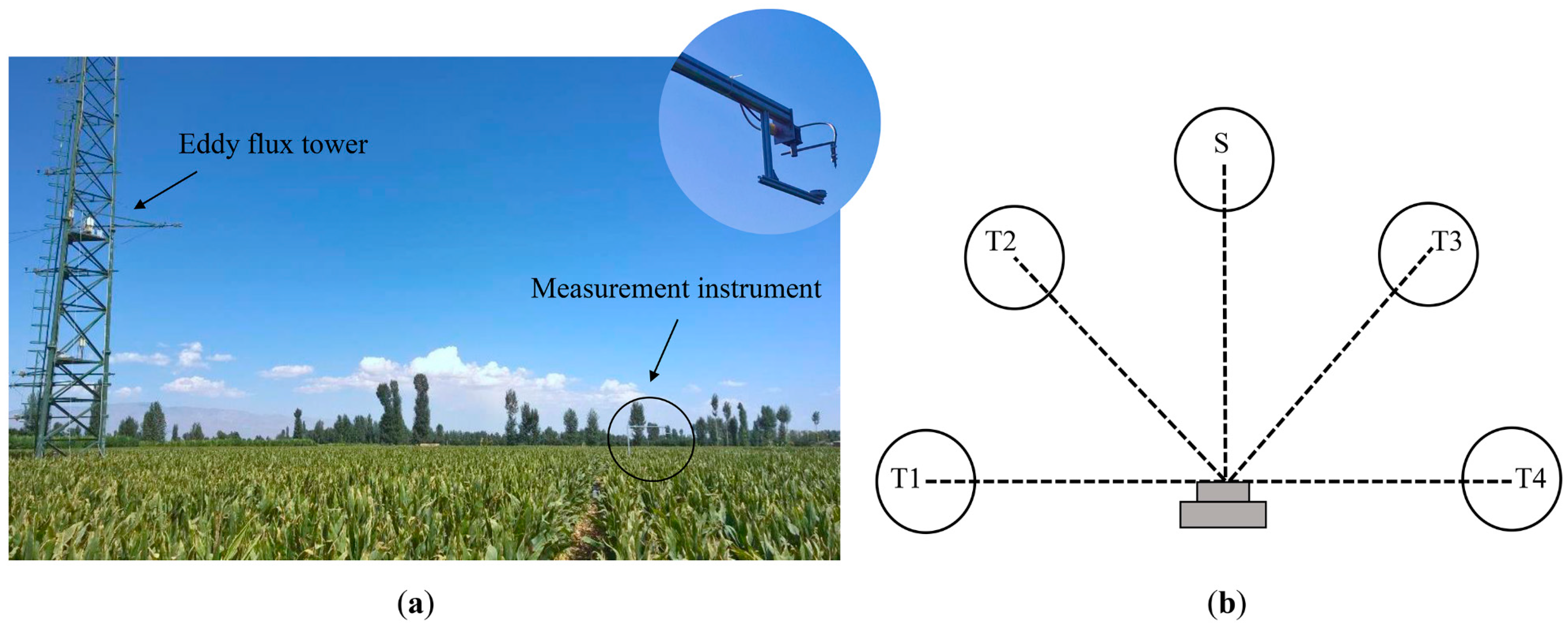
2.1. Study Site Description

A field experiment was conducted near an eddy flux tower in the Zhangye oasis irrigation area located in the middle of the Heihe watershed, northwestern China (100.372°E, 38.856°N, altitude 1556 m) (Figure 1). This station was funded in May 2012 with the support of the Heihe Watershed Allied Telemetry Experimental Research (HiWATER) (http://westdc.westgis.ac.cn/data) [50,51]. It was dominated by maize during our experimental period. The research area is characterized by a mean annual temperature of 6 °C and a mean annual precipitation of 114.9 mm, which falls mostly from June to September. During our campaign, the average height of the canopy was approximately 1.8 m.

2.2. Eddy Covariance Measurements

The EC system that was installed within our study area collected continuous measurements beginning on 25 May 2012. It consisted of a three-dimensional sonic anemometer (CSAT3, Campbell Scientific Inc., Logan, UT, USA) and an open path CO2/H2O analyzer (LI7500A, LI-COR Biosciences, Lincoln, NE, USA). The anemometer measured the three-dimensional wind velocity and temperature, and the CO2/H2O analyzer monitored the CO2/H2O density. Both sensors were placed 4.5 m above the ground and separated 17 cm away from each other in the horizontal direction. They were connected to a data logger (CR1000, Campbell Scientific Inc., Logan, UT, USA) that recorded the measurements with a sampling frequency of 10 Hz. The EC measurements were processed to half-hourly averages using the EddyPro software package [50,51].
Measurements of air temperature and relative humidity were taken close to the EC system at seven heights (3 m, 5 m, 10 m, 15 m, 20 m, 30 m, and 40 m). All data were processed to 10 min intervals [51]. To match the EC measurements, we used measurements at a height of 5 m in this research.
The diurnal courses of GPP (mg m−2 s−1) during our experiment period were obtained by partitioning the observed net ecosystem exchange (NEE) into GPP and ecosystem respiration (Re) according to Coops et al. [52] and Zhang et al. [53].

2.3. Field Data Collection
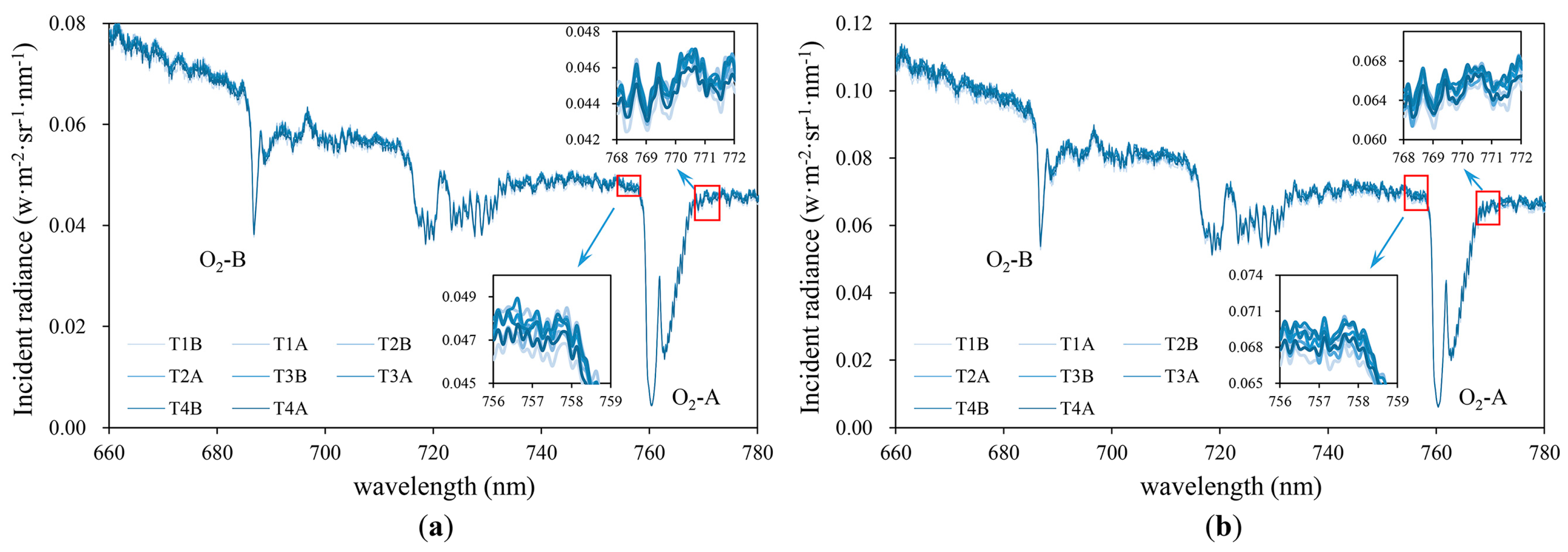
Spectral measurements at the canopy level were carried out under clear-sky conditions in July and August 2015, when the maize plants were at the late big trumpet period and the ripening stage, respectively. The vegetation fraction during our campaign is greater than 0.8. A calibrated HR4000 high-resolution spectroradiometer (Ocean Optics Inc., Dunedin, FL, USA) was installed at approximately 20 m from the eddy flux tower to measure the diurnal cycles of the canopy radiometric response (Figure 2a). It records reflected radiation within the spectral domain of 647–1087 nm with a full width at half maximum (FWHM) bandwidth of 0.13 nm. During our experiment, the spectroradiometer was housed in a thermally regulated box (SteadiQ, Ocean Optics Inc., Dunedin, FL, USA) and the internal temperature was maintained at 25 °C to reduce dark current drift. Spectralon reflectance standards (WS-1-SL, Ocean Optics Inc., Dunedin, FL, USA) were used to measure the incident irradiance.
For the canopy measurements, the instrument’s fiber optic was attached to a swiveling mount that was elevated approximately 1 m above the canopy and adjusted for nadir view. The daily cycles of the reflectance spectra under clear sky conditions at four different canopy locations were collected in our campaign. As the FOV (Field of View) of the instrument is 25°, each measurement can acquire a circle area of 0.5 m in diameter (Figure 2b). During the measurement, the swiveling mount was manually controlled to acquire sequential observations of the standard reference panel and the canopy targets. Specifically, each acquisition session consisted of the consecutive collection of spectra of instrument dark current, radiance of the standard reference panel, canopy radiance and radiance of the standard reference panel. After acquiring the radiance of the standard reference panel, the fiber optic was immediately switched to the canopy target to acquire canopy radiance. Then the fiber optic was switched to the standard reference panel to acquire its radiance again. The radiance of the standard reference panel at the time of the canopy measurement was determined using the averaged spectrum of the two measurements. To ensure high-quality spectral data, ten consecutive spectra were averaged as a single spectrum at each measurement. The integration time was automatically optimized during the day to maximize the signal-to-noise ratio (SNR). In the experiment, the spectral acquisitions were conducted at 0.5 h intervals. Eventually, five diurnal courses of reflectance spectra were acquired (Table 1).
In addition to the spectral measurements, the absorbed photosynthetically active radiation (APAR) was collected simultaneously within 10 m away the FOV of the spectrometer using an LI-190SA quantum sensor (LI-COR Biosciences, Lincoln, NE, USA) that measures PAR in the range of 400–700 nm. APAR acquisition is based on the measurements of four radiation components: PAR reaching the canopy, PAR reflected from the canopy, PAR transmitted through the canopy, and PAR reflected from the ground. APAR was determined by referring to Gallo and Daughtry [54].
During our campaign, LAI was measured twice at 18 July and 22 August, respectively. Each measurement was conducted shortly after sunset using an LI-2200 plant canopy analyzer (LI-COR Biosciences, Lincoln, NE, USA). The measurements were conducted within a 10 m × 10 m area around the spectral measurement instrument. The measurement at 18 July with value of 3.97 was used for all the July studies, and the measurement at 22 August with value of 4.22 was used for all the August studies, respectively.

2.4. SIF Retrival

Chlorophyll fluorescence is the re-emission of solar radiation absorbed by leaf chlorophyll at longer wavelengths, and it has a distinct spectral shape with one peak at 685–690 nm (red fluorescence) that is mainly attributed to the fluorescence emission of photosystem II (PSII) and another at 730–740 nm (far-red fluorescence) that is attributed to both PSI and PSII [34]. The solar-induced fluorescence (SIF) adds a weak signal to the reflected solar radiation. Depending on the wavelength, the amount of SIF that is emitted by the canopy is approximately 8.7–21.9% and 2–5.2% of the total reflected light at 685 nm and 740 nm, respectively [25,55,56].
The SIF signal is usually discriminated using the Fraunhofer lines in which irradiance is strongly reduced [57,58]. Three Fraunhofer lines are generally used in the visible and near-infrared region: Hα line (centered at 656.4 nm) due to hydrogen absorption in the solar atmosphere, O2-A (centered at 760.4 nm) and O2-B (centered at 687 nm) due to telluric oxygen absorption in the atmosphere [59,60,61]. As PSI emits fluorescence only in the near-infrared part of the fluorescence spectrum and PSII emits over a wide spectrum and peaks in the red part, the two oxygen absorption lines that corresponded with the two fluorescence emission peaks can be used to obtain SIF signal emitted mainly by PSI and PSII, respectively [34]. Previous studies have demonstrated that red SIF is affected by the reabsorption of leaf chlorophyll and LAI variations, which causes a lower correlation between red SIF and GPP when compared with the far-red SIF [36,62]. Thus, we mainly consider the far-red SIF in this study.
Almost all SIF retrieval algorithms are based on the Fraunhofer line depth (FLD) principle that was originally proposed by Plascyk [57] and Plascyk and Gabriel [58]. The principle assumes that the reflectance signal and the SIF signal within and outside the dark line remain constant (see the review written by Meroni et al. [59]).
In this study, we used the O2-A line to obtain the far-red SIF (SIF760) according to the modified FLD method proposed by Maier et al. [63]. This approach, which is referred to as 3FLD, assumes that the variations in the SIF and reflectance signals are linear. The signals at three bands, including one within the absorption valley and two outside the valley, are used to derive the SIF. The weights of the two outside channels are defined as
w left = λ right λ in λ right λ left
and
w right = λ in λ left λ right λ left
where λleft and λright indicate the shorter and longer wavelengths adjacent to the absorption valley, respectively. The SIF can be generated using
S I F = ( E left w left + E right w right ) L in E in ( L left w left + L right w right ) ( E left w left + E right w right ) E in
where E and L represent the ground irradiance and the canopy radiance, respectively.
Former studies have indicated that the 3FLD algorithm can generate reliable SIF signals when used on datasets obtained using the aforementioned HR4000 (SR = 0.13 nm, SNR > 300) [64,65]. Therefore, we considered the derived SIF to be suitable for our research.

2.5. Statistical Analysis of the SIF-GPP Relationship

According to the LUE theory proposed by Monteith [66], the GPP can be obtained by
G P P = A P A R × L U E P
where APAR represents the absorbed photosynthetically active radiation and LUEP refers to the efficiency in which APAR is used in photosynthesis.
As a by-product of photosynthesis, SIF can be similarly expressed as
S I F = A P A R × L U E F × f esc
where LUEF is the light-use efficiency for SIF, which represents the fraction of APAR that is re-emitted from the canopy as SIF photons and fesc is the fraction of SIF photons escaping the canopy [24].
By combining Equations (4) and (5), SIF can be theoretically linked with GPP as
G P P = S I F × L U E P L U E F × f esc S I F × L U E P L U E F
where fesc ≈ 1 can be assumed to be due to the low absorptance of leaves in the far-red wavelengths and the relatively simple plant structure and high leaf area index of crops [24,67].
As shown in Equation (6), if the LUEP/LUEF ratio is constant, the SIF would be a good constraint used to determine GPP regardless of changes in the APAR or stresses. Previous studies have demonstrated that these two terms (LUEP and LUEF) covary in most cases, and the ratio of one to the other tends to be constant under high light conditions, which makes it possible to establish a linear statistical model between SIF and GPP [23,25,68]. In this study, we generated a statistical model to assess the ability of SIF to estimate GPP.

2.6. MuSyQ-GPP Algorithm

The MuSyQ-GPP algorithm was designed as part of the multi-source data synergized quantitative (MuSyQ) remote sensing production system [12]. It presents an LUE approach to model the GPP using remotely sensed data and meteorological data with different spatial and temporal resolutions. The algorithm was adopted to generate the GPP at the site level in this research.
The MuSyQ-GPP algorithm estimates GPP using the LUE theory described in Equation (4). It employs down-regulating scalars to characterize the effects of temperature and water stress on the LUEP as
L U E P = L U E 0 × f 1 ( T ) × f 2 ( β )
where LUE0 is the potential or maximum LUEP (gC mol−1 PPFD), and f1(T) and f2(β) represent the down-regulation effects of temperature and water conditions on LUE0, respectively. A theoretical LUE0 value of 0.60 gC mol−1 PPFD that was reported in a previous study [69] was used in this study.
The temperature-limited effect on LUE0 is generated using two terms, T1 and T2
f 1 ( T ) = T 1 × T 2
where
T 1 = 0.8 + 0.02 T opt 0.0005 T opt 2
T 2 = 1.1814 / { [ 1 + e 0.2 ( T opt 10 T ) ] [ 1 + e 0.3 ( T opt 10 + T ) ] }
where Topt represents the optimum temperature, which is defined as 28 °C in our study as in Kalfas et al. [70]
The limited effect of water conditions on plant photosynthesis, which ranges between 0.5 and 1, is derived following the algorithm
f 2 ( β ) = 0.5 + 0.5 E / E P
where E and EP represent the actual and potential evapotranspiration, respectively.
In the MuSyQ-GPP algorithm, a modified Penman–Monteith (P-M) approach with biome-specific canopy conductance [71,72,73,74] is used to estimate the actual evapotranspiration (see Text S1 in Supplementary Materials). The potential evapotranspiration is calculated using the Priestley and Taylor (P-T) equation [75].
The original version of the MuSyQ-GPP model was established to estimate the daily GPP over regional and global scales [12]. In our study, we deployed its original algorithms to generate half-hourly averaged GPP at the site level to evaluate the performance of the LUE model.

2.7. BEPS Approach

The BEPS model used in our study is an hourly process-based diagnostic model [13,14,76] that computes the canopy level GPP as the sum of the sunlit and shaded leaf groups using the Farquhar, von Caemmerer and Berry (FvCB) photosynthesis model [18]. Although the BEPS was initially developed for boreal ecosystems, it has been expanded and used for temperate and tropical ecosystems in Asia [77,78], which laid the foundation for its application in croplands.
The BEPS adopts a sunlit-shaded leaves separation modeling mechanism that upscales photosynthesis from the leaf level to the canopy level. This kind of “two-leaf” model has been proven to be more effective in modeling canopy photosynthesis than the conventional “big-leaf” model [13,79]. The photosynthetic rate of the canopy, Ac, is modeled as the sum of the sunlit and shaded leaf groups as
A c = A sunlit L A I sunlit + A shaded L A I shaded
L A I sunlit = 2 cos θ ( 1 e 0.5 Ω L A I / cos θ )
L A I shaded = L A I L A I sunlit
where sunlit and shaded denote the sunlit and shaded leaf groups, respectively; θ is the solar zenith angle; and Ω is the clumping index.
The photosynthesis model in the BEPS model is suitable for C3 carbon fixation pathways. However, maize is a C4 species according to its photosynthetic pathway. In this study, the BEPS model was modified to be suitable for C4 species estimation according to the theory of Collatz et al. [19]. The photosynthetic rate of the leaves for C4 species, An, is assumed to be limited by the phosphoenolpyruvate carboxylase (PEP-carboxylase)-limited rate of assimilation (Wc), the light-limited rate of assimilation (We), and the CO2-limited rate of assimilation (Ws) [80]
A n = min ( W c , W e , W s ) R d
W c = V cmax
W e = P A R × ( 1 ω ) × ε
W s = 2 × 10 4 V cmax C i / p
R d = 0.0025 V cmax
where Vcmax is defined as the maximum carboxylation rate (mol m−2 s−1), ω is the leaf-scattering coefficient for PAR, ε represents the intrinsic quantum efficiency of CO2 uptake (mol mol−1), and Rd is the leaf dark respiration rate (mol m−2 s−1).
The C4 photosynthesis model was integrated into the BEPS model to couple with the Ball-Berry stomatal conductance model to generate the photosynthesis rate using an iteration calculating procedure [19,81].

3. Results

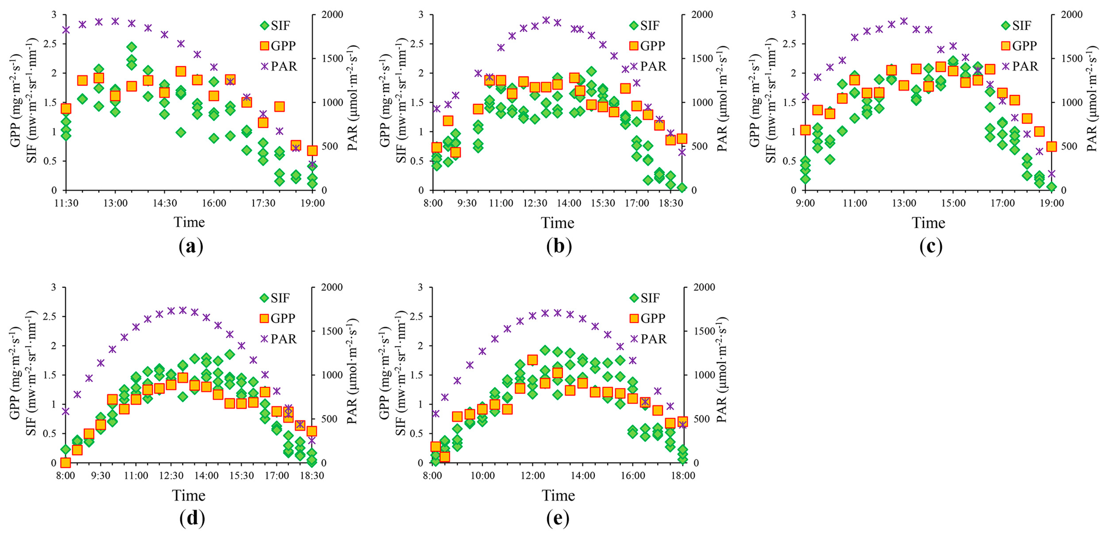
3.1. Diurnal Patterns in GPP and SIF760

The diurnal courses of GPP, SIF760, and PAR during our campaign are shown in Figure 3. Since the canopy spectra were collected at four different positions, four SIF760 values together with one GPP value were obtained at a time. As shown in Figure 3, both SIF760 and GPP exhibit similar patterns to that of PAR with lower values in the early morning and late afternoon and higher values in the middle of the day. These values tend to exhibit a single peak curve that follows the variation of PAR. The distinct decrease in GPP at midday that is commonly found in C3 species, known as the “midday depression”, was not observed in our experiment, which is consistent with the studies by Cheng et al. [82] and Liu et al. [25] For C3 species, higher temperatures can decrease the affinity of enzymes for CO2 and cause the carboxylation enzyme, Rubisco, to be less active, which leads to the midday reductions in carbon assimilation. In addition, the higher evaporative demands at midday reduces the stomatal conductance, which also affects the assimilation rate. In contrast, for C4 species, CO2 is delivered to Rubisco, which is localized in the bundle sheath chloroplasts, by a metabolic pump that concentrates CO2 [19]. This mechanism can inhibit photorespiration and promote carbon assimilation. Consequently, C4 species exhibit higher photosynthesis capacities at high temperatures where photorespiration is stimulated. In addition, C4 species generally have lower stomatal conductance than C3 species [19]. Lower conductance coupled with higher photosynthetic capacity in C4 species results in higher water use efficiencies in comparison to C3 species. The similar pattern between SIF760 and PAR indicates the capacity of SIF in protecting plant tissues from light energy that may be excessive for photosynthesis and could otherwise damage tissues. Although some research has demonstrated that SIF will increase with PAR at low light then decrease when NPQ increases and further increase when NPQ reaches saturation [83], we did not find this kind of variation clearly in our experiment. Actually, only one set of data on 17 July showed slight decreases at approximately 11:30 and 14:30, which might correspond to the aforementioned decreasing trend. However, we also noticed that the SIF760 values of the four canopy positions had relatively higher diversity on 17 July (as well as 10 July) than on the other days. It is not clear whether it can to be attributed to the NPQ increment or observation bias. Thus, further studies are needed, and both data quality and quantity should be considered before drawing such a conclusion. For our study, we found that SIF760 showed a pattern with a single peak that followed the variation of PAR as concluded by Liu et al. [25].
We also analyzed the relationships between APAR and both SIF760 and GPP. Both showed strong linear correlations, and an R2 of 0.713 (Figure 4a) and 0.591 (Figure 4b) was achieved between APAR and SIF760 and APAR and GPP, respectively. The averaged SIF760 values were also generated to reduce some uncertainties introduced during our spectral acquisition. As our measurements were conducted at four different canopy positions, we assumed their mean values could adequately represent the situations of our study site. By analyzing the relationship between APAR and the averaged SIF760, the R2 increased to 0.798 (Figure 4c). As illustrated in Figure 4, the slope of the SIF760-APAR relationship is approximately the same LUEF, and the slope of the GPP-APAR relationship can be considered as LUEP. Because both relations can be adequately expressed by linear equations, the ratio between LUEP and LUEF, as described in Equation (6), can be considered nearly constant, which means that SIF760 and GPP can be directly linked.

3.2. Relationship between SIF and GPP

Statistical analysis was conducted to reveal the relationship between SIF760 and GPP. As shown in Figure 5, we found a significant correlation between SIF760 and GPP, and their relationship could be characterized by a linear function, regardless of using individual SIF760 of the four group measurements (GPP = 0.570 × SIF760 + 0.666) or the averaged measurements (GPP = 0.621 × SIF760 + 0.614), which suggests that SIF760 can be used as a direct proxy for GPP.

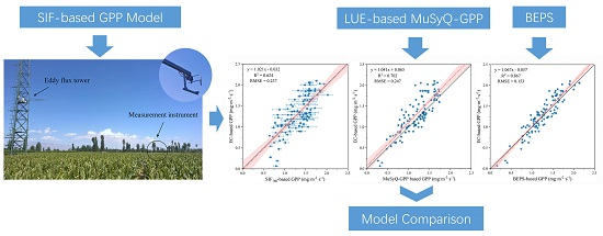
3.3. Comparison of GPP Modeled by SIF, MuSyQ-GPP, and BEPS Models

In addition to the SIF-based GPP estimation, we also generated GPP using both the LUE-based MuSyQ-GPP algorithm and the process-based BEPS model. As the BEPS model used in our study was initially designed to run at hourly intervals, we modified it to a half-hourly time step to match the observations in this study. Thus, all approaches were performed every 30 min in our analysis. As the average of the four SIF760 measurements may represent the situations of our study site better than the individual measurements, we only considered the statistical model generated using the averaged SIF760 values (GPP = 0.621 × SIF760 + 0.614) in this study. As shown in Figure 6, all three approaches estimate the GPP well. Among which, the BEPS model (R2 = 0.867, RMSE = 0.153 mg m−2 s−1) performs better than that of SIF760 (R2 = 0.624, RMSE = 0.237 mg m−2 s−1) and MuSyQ-GPP (R2 = 0.702, RMSE = 0.247 mg m−2 s−1) models. We also modeled GPP using the statistical model generated with SIF686 (GPP = 0.682 × SIF686 + 0.539) (see detailed results in Text S2, Figures S1–S4 in Supplementary Materials). Compared with the SIF760-based model, SIF686-based GPP model showed a limited accuracy with R2 = 0.456 and RMSE = 0.363 mg m−2 s−1.
We noticed that some of the SIF-based GPP estimates were higher than the EC-based estimates when GPP was relatively low, which corresponded to the observations at 8:30 on 21 August and 8:30 on 22 August (dots in the red circle in Figure 6a). When these two groups of data were excluded from the analysis, both SIF based GPP models performed better with R2 increased to 0.667 and RMSE decreased to 0.236 mg m−2 s−1 for the SIF760-based model, and R2 increased to 0.459 and RMSE decreased to 0.352 mg m−2 s−1 for the SIF686-based model, respectively. The MuSyQ-GPP algorithm was found to underestimate the GPP values at high productivity, which could be attributed to the assignment of a constant LUE0 value in the algorithm as it could not properly handle the contribution of both sunlit and shaded leaves to the total GPP. BEPS model was found to slightly underestimate GPP at high productivity and overestimate GPP at low productivity. Among these three approaches, BEPS model showed better performance than that of SIF-based or LUE-based MuSuQ-GPP models, with higher R2 and lower RMSE.

4. Discussion

4.1. Uncertainties in the SIF Measurements

The SIF retrieval accuracy is dependent on the spectral characteristics of the reflectance and irradiance spectra around the oxygen absorption lines. According to our validation based on EC-based data, the SIF760-based GPP at 8:30 on 21 August and 8:30 on 22 August deviate from the EC-based values significantly (dots in the red circles in Figure 6). During our experiment, we measured four canopy positions sequentially from T1 to T4 as illustrated in Figure 2. The spectra of the reference panel were collected eight times: once before and once after each of the four canopy measurements. Incident radiance at 8:30 on 21 August and 8:30 on 22 August was then obtained (Figure 7). The incident radiance showed significant variations during our measurement, especially at the left and right shoulders of the absorption line. Additionally, the measured irradiance did not present a gradual increase trend as expect. This may be attributed to the instability of irradiance in the morning. As light travels a longer path at high solar zenith angle (SZA) in the morning, the influence of atmospheric conditions would be larger than that at lower SZA. Hence, in future studies, it is necessary to consider the influence of air conditions and the affection of imaging geometrical conditions such as the SZA and relative azimuth angle in SIF retrieval.
The data quality (DQ) indicator DQs presented by Cogliati et al. [84] was adopted to evaluate the stability of the incident radiance. DQs is defined as the percentage of variation between the first and the second irradiance measurement
D Q s = | E B E A | / E B × 100
where EB and EA represents the incident radiance before and after the canopy measurement, respectively.
In this study, the DQs values of the three bands used in the 3FLD algorithm were averaged to represent the irradiance stability. As shown in Figure 8, the DQs values were generally higher at morning and evening and lower at noon, the higher values also corresponded with the higher SZA and longer path. For the observations at 8:30 on 21 August and 8:30 on 22 August, the DQs showed the largest values, which indicated that the irradiance changed significantly during these measurement sessions. Therefore, data quality check is needed especially when irradiance demonstrates significant variations, the acquisition that do not meet the quality check should be rejected and no longer considered in the analyses.
We used the 3FLD algorithm to generate SIF in this study. The 3FLD approach is based on the assumption that the reflectance signal and the SIF signal vary linearly within and outside the absorption band. However, the actual variations of reflectance and SIF signal are not being linear, which causes a violation of the underlying assumption of the 3FLD method and lead to some uncertainties in SIF retrieval. Additional studies are needed in generating SIF with more advanced SIF retrieval approaches such as the improved FLD (iFLD) method [85] or the Spectral Fitting Methods (SFM) [86].

4.2. Uncertainties in the SIF-Based GPP Model

Previous studies have demonstrated that the relationship between remotely sensed SIF and GPP can be characterized by a linear and ecosystem-specific function [23,24,25]. There is also evidence indicating that the SIF and GPP relationship can be affected by various factors such as the rate of NPQ [61,87], light conditions [46,87], nutrient availability [61], water availability [87], temperature [23,46,68], and canopy structure [34]. Recent studies have suggested that there is a curvilinear relationship between instantaneous SIF and GPP due to the rate of photosynthesis saturated under high illumination, and this relationship tends to become linear when both SIF and GPP are temporally aggregated [28,34]. However, the saturation of GPP with APAR were not found in our experiment (Figure 4) as C4 species exhibit higher photosynthesis capacities at higher temperatures than C3 species. Therefore, the relationship between SIF and GPP could be adequately characterized by a linear function in our research. However, the SIF-GPP relationship may not be constant in spatial and temporal modeling, which can be attributed to the ecosystem-specific structural and physiological characteristics as well as the environmental situations associated with each ecosystem [34]. Therefore, for accurate quantification and characterization of the SIF-GPP relationship, further experiments that overlap the entire growth periods in various ecosystems are needed, especially for C3 species.
Remote measurements of SIF are likely representative of the upper layer of the canopy, which is mainly characterized by sunlit leaves [34,59]. Although the upper layer substantially contributes to the total GPP, there are still many layers of leaves that contribute to the canopy photosynthesis at different rates depending on their sunlit or shaded exposure [59]. Thus, the heterogeneity of the vertical canopy may lead to a mismatch between the SIF-based estimates and the EC-based GPP. Additionally, under low light unstressed conditions, there exists a competitive relationship between leaf fluorescence and photosynthesis and a positive correlation between them under stressed and high light conditions [87,88]. The relationships between SIF and GPP for sunlit and shaded leaves are different as sunlit leaves receive more light and shaded leaves only receive diffuse light [88]. Therefore, additional studies are needed to address the contributions of the shaded leaf groups and the structural sensitivities of canopy-leaving SIF signals.
Light energy absorbed by leaf chlorophyll molecules has three different pathways: photochemistry, NPQ, and SIF. Accurately estimating any one of the de-excitation pathways require measurement of the other two. Some researches indicated that most absorbed energy is used in photosynthesis and both fluorescence and NPQ are low under low light conditions. Under high light and stressed conditions, NPQ becomes dominant and the yields of fluorescence and photosynthesis decrease [87]. As a result, the relationship between SIF and GPP is influenced by NPQ. The mechanism of NPQ and its regulation should be considered in the further studies.
Plant photosynthesis starts with absorption of light, mainly by chlorophyll molecules. Accordingly, some mechanisms were used to modulate photosynthetic light. Former studies have indicated that chloroplasts can change their orientation within the cell in response to the intensity and direction of the incident light [89]. When light is limiting to photosynthesis, chloroplasts move to positions that yielding maximum light absorption, whereas in saturating light they hide themselves to make the light absorption minimized. The chloroplast avoidance movements can lead to decreased light absorption and then influence the observed SIF signal, and further studies are needed. Additionally, leaf movements and leaf angle adjustments can also significantly affect the fractions of sunlit and shaded leaves, which should be considered in future research.
The mismatches of the spatial and temporal scales between canopy SIF and EC-based GPP also lead to some uncertainties. The footprint of the EC tower covers 0.01 km2 to 10 km2 depending on the measurement height, wind speed and turbulent state of atmosphere [90], whereas the canopy SIF are instantaneously measured with a footprint less than one square meter.
The availability, quality, and spatiotemporal coverage of SIF data are expected to increase drastically over the next few years. SIF measurements have been conducted at ecosystem, landscape, and global scales using field spectroradiometers, airborne instruments, and satellite platforms, respectively. The NASA’s OCO-2 [43], ESA’s Sentinel-5 Precursor (TROPOMI) [91] and ESA’s Earth Explorer Fluorescence Explorer (FLEX) [92,93] can provide SIF data at much higher spatial resolutions. In particular, the FLEX mission can provide auxiliary information such as NPQ and canopy temperature along with fluorescence information. These data would improve our estimation of the global carbon budget and our ability to track the health of terrestrial ecosystems. Additionally, the development of the SCOPE (Soil-Canopy Observation, Photosynthesis and Energy balance) model provides a theoretical way to model canopy SIF and photosynthesis by combing Soil-Vegetation-Atmosphere-transfer (SVAT) model with radiative transfer models [94]. Despite this promising scenario and the empirical evidence that SIF provides novel information to estimate photosynthesis, as found in our study, there are still many uncertainties in relating SIF and GPP, and further studies are needed.

4.3. Limitations of the LUE-Based Model

The basis of the LUE-based models is the initial linear relationship between the GPP and APAR of the canopy [63]. However, this relationship is not linear at the individual leaf level and is characterized by temporal heterogeneity associated with the variation of illumination levels [95]. Photosynthesis in sunlit leaves is often light-saturated and limited by the level of Rubisco activity related to leaf nutrient conditions and the ambient temperature [18], which results in a lower LUE, while photosynthesis in shaded leaves is often not light-saturated and essentially has a linear response to APAR, which results in a higher LUE [13,96,97,98,99]. In the LUE-based MuSyQ-GPP algorithm, LUE is determined by assigning a constant maximum value of LUE0 and adjusting downward based on temperature and water conditions. Daily variability in the sunlit and shaded leaf fractions cannot be represented in this model. Consequently, the internal physiological processes of these two leaf groups are substantially different and the LUE of the shaded leaves is generally higher than that of the sunlit leaves [95]. As GPP can vary greatly in space and time as a result of the variability between sunlit and shaded leaf fractions, we argue that scaling the LUE0 without considering the difference between the sunlit and shaded leaf groups can significantly limit the performances of the LUE-based models. There are some literature suggests that the LUE models underestimate GPP at high productivity and overestimate GPP at low productivity [96], and the underestimation is consistent with our research. However, the overestimation cannot be clearly shown in our analysis. These results are not contradictory since our data at low productivity is limited. In addition, the LUE0 used in the LUE-based models is usually defined as a constant value for each broadly defined plant functional type (PFT). For our study, we used a constant value of 0.60 gC mol−1 PPFD from the study by Zhang [69], which was conducted at the same site as our study. However, other literature has suggested that LUE0 for maize at different sites can be assigned as 1.50 gC mol−1 PPFD [67,100], 0.93 g C mol−1 PPFD [101], or 1.22 g C mol−1 PPFD [101]. Therefore, LUE0 varies among vegetation types and study sites and should be calibrated before using in the LUE-based approach. Moreover, the MuSyQ-GPP algorithm deploys two down-regulating factors to represent the effects of temperature and water conditions while scaling the LUE0. Although various strategies have been developed to characterize the impacts of temperature and water stresses [8,9,10,11], the descriptions of their influences in the LUE-based approaches are still empirical, which may introduce some uncertainties, especially for the water stress scalar. For the MuSyQ-GPP algorithm, a calculation of evapotranspiration is conducted to represent water availability. Predictably, the uncertainties existing in the evapotranspiration estimation would lead to significant deviations in the final GPP estimation.

4.4. Uncertainties in the BEPS Model

The core idea of the BEPS model is that it adopts separate sunlit and shaded leaves modeling mechanisms. The two-leaf model has been proven to be more efficient in simulating the daily variation of canopy photosynthesis than the conventional “big-leaf” model [13]. The BEPS model employs the enzyme kinetics theory for C3 plants proposed by Farquhar et al. [18] to generate the photosynthesis rate. In this study, we adopted a modified version that was applicable for C4 species [19] and integrated it into the BEPS model to couple with the Ball-Berry stomatal conductance model [81] to generate GPP as well as the water and heat fluxes. Although it is designed in an explicit and tightly linked manner that simulates the coupled hydrological, ecophysiological, and biogeochemical processes and the associated feedback mechanisms, it should be noted that numerous parameters should be assigned before modeling. One of the most important parameters in modeling photosynthesis, the maximum carboxylation rate (Vcmax in Equations (16), (18), and (19)), has been proven to vary temporally [48,102,103,104], although it is usually assigned as a specific value for each PFT [105]. In this study, we adopted a constant value of 37 μmol m−2 s−1 by referring to Zhang et al. [48]. Although BEPS model simulated GPP better than the SIF-based and LUE-based model in our study, there are still some underestimations at high productivity and overestimations at low productivity. Therefore, additional studies are needed in generating the seasonal variation of Vcmax. Former studies have demonstrated that Vcmax can be related with reflectance [106] or leaf chlorophyll content [107], which made it retrievable using remotely sensed data. Recently, a study conducted by Zhang et al. [48] presented an SIF-based approach for modeling seasonal Vcmax, which provided a new method to assess plant photosynthesis using SIF.

5. Conclusions

In this study, we evaluated the ability of three different approaches, SIF, LUE-based MuSyQ-GPP, and process-based BEPS, to estimate the diurnal courses of GPP at a maize site. In general, all three approaches adequately estimated the GPP, and the process-based BEPS model had the best performance, followed by the LUE-based MuSyQ-GPP algorithm and the SIF-based statistical model. The MuSyQ-GPP algorithm underestimated the GPP at high productivity, which can be attributed to its weakness in characterizing the underlying ecological processes of vegetation and the contribution of shaded leaves to total GPP. In contrast, the BEPS model that was established based on the two-leaf theory and physiological mechanisms can provide more accurate estimations. Our study indicated that the SIF760-based statistical model can provide reasonable estimates of GPP in the short term without additional information such as climate inputs, which are required by the process-based and LUE models.
The observational approach revealed that both SIF760 and GPP exhibited similar diurnal patterns as PAR, both SIF760 and GPP were linearly correlated with APAR, and a linear function could well characterize the relationship between SIF760 and GPP for maize over our study period. Despite its limitations in applying to large area and long-term studies, SIF provided a proxy for GPP not available from any other remote sensing measurements of vegetation.

Supplementary Materials

The following are available online at www.mdpi.com/2072-4292/9/12/1267/s1, Text S1: Estimation of water stress factor in the MuSyQ-GPP algorithm, Text S2: Performance of the SIF686-based GPP model, Figure S1: Diurnal patterns of PAR, GPP and SIF686 during the experiment, Figure S2: Relationship between APAR and individual SIF686 and averaged SIF686, Figure S3: Relationship between individual SIF686 and GPP, averaged SIF686 and GPP, Figure S4: Relationships between SIF686-based GPP and EC-based GPP during the experiment period.

Acknowledgments

This work was supported by the National Key R&D Program of China (2017YFA0603002) and the National Natural Science Foundation of China (61661136006001, 41471349, and 41531174). We would like to thank Jingming Chen and Gang Mo from University of Toronto for providing the BEPS model.

Author Contributions

Tianxiang Cui, Rui Sun and Zhigang Liu conceived and designed the experiments; Tianxiang Cui, Chen Qiao, Qiang Zhang, Tao Yu and Gang Liu implemented the experiments; Tianxiang Cui preprocessed and analyzed the data; and Tianxiang Cui and Rui Sun prepared the paper.

Conflicts of Interest

The authors declare no conflict of interest.

References

  1. Melillo, J.M.; Mcguire, A.D.; Kicklighter, D.W.; Moore, B.; Vorosmarty, C.J.; Schloss, A.L. Global Climate-Change and Terrestrial Net Primary Production. Nature 1993, 363, 234–240. [Google Scholar] [CrossRef]
  2. Thurner, M.; Beer, C.; Santoro, M.; Carvalhais, N.; Wutzler, T.; Schepaschenko, D.; Shvidenko, A.; Kompter, E.; Ahrens, B.; Levick, S.R.; et al. Carbon stock and density of northern boreal and temperate forests. Glob. Ecol. Biogeogr. 2014, 23, 297–310. [Google Scholar] [CrossRef]
  3. Baldocchi, D. Breathing of the terrestrial biosphere: Lessons learned from a global network of carbon dioxide flux measurement systems. Aust. J. Bot. 2008, 56, 1–26. [Google Scholar] [CrossRef]
  4. Goulden, M.L.; Munger, J.W.; Fan, S.M.; Daube, B.C.; Wofsy, S.C. Measurements of carbon sequestration by long-term eddy covariance: Methods and a critical evaluation of accuracy. Glob. Chang. Biol. 1996, 2, 169–182. [Google Scholar] [CrossRef]
  5. Long, S.P.; Bernacchi, C.J. Gas exchange measurements, what can they tell us about the underlying limitations to photosynthesis? Procedures and sources of error. J. Exp. Bot. 2003, 54, 2393–2401. [Google Scholar] [CrossRef] [PubMed]
  6. Prieto-Blanco, A.; North, P.R.J.; Barnsley, M.J.; Fox, N. Satellite-driven modelling of net primary productivity (npp): Theoretical analysis. Remote Sens. Environ. 2009, 113, 137–147. [Google Scholar] [CrossRef]
  7. Zhang, Y.; Xiao, X.M.; Jin, C.; Dong, J.W.; Zhou, S.; Wagle, P.; Joiner, J.; Guanter, L.; Zhang, Y.G.; Zhang, G.L.; et al. Consistency between sun-induced chlorophyll fluorescence and gross primary production of vegetation in North America. Remote Sens. Environ. 2016, 183, 154–169. [Google Scholar] [CrossRef]
  8. Potter, C.S.; Randerson, J.T.; Field, C.B.; Matson, P.A.; Vitousek, P.M.; Mooney, H.A.; Klooster, S.A. Terrestrial ecosystem production—A process model-based on global satellite and surface data. Glob. Biogeochem. Cycles 1993, 7, 811–841. [Google Scholar] [CrossRef]
  9. Prince, S.D.; Goward, S.N. Global primary production: A remote sensing approach. J. Biogeogr. 1995, 22, 815–835. [Google Scholar] [CrossRef]
  10. Xiao, X.M.; Zhang, Q.Y.; Braswell, B.; Urbanski, S.; Boles, S.; Wofsy, S.; Berrien, M.; Ojima, D. Modeling gross primary production of temperate deciduous broadleaf forest using satellite images and climate data. Remote Sens. Environ. 2004, 91, 256–270. [Google Scholar] [CrossRef]
  11. Running, S.W.; Zhao, M.S. User’s Guide. Daily GPP and Annual NPP (MOD17A2/A3) Products NASA Earth Observing System MODIS Land Algorithm; Version 3.0 for Collection 6. Available online: https://lpdaac.usgs.gov/sites/default/files/public/product_documentation/mod17_user_guide.pdf (accessed on 6 December 2017).
  12. Cui, T.; Wang, Y.; Sun, R.; Qiao, C.; Fan, W.; Jiang, G.; Hao, L.; Zhang, L. Estimating vegetation primary production in the Heihe river basin of China with multi-source and multi-scale data. PLoS ONE 2016, 11, e0153971. [Google Scholar] [CrossRef] [PubMed]
  13. Farquhar, G.D.; von Caemmerer, S.; Berry, J.A. A biochemical model of photosynthetic CO2 assimilation in leaves of c 3 species. Planta 1980, 149, 78–90. [Google Scholar] [CrossRef] [PubMed]
  14. Collatz, G.J.; Ribas-Carbo, M.; Berry, J.A. Coupled photosynthesis-stomatal conductance model for leaves of C4 plants. Aust. J. Plant Physiol. 1992, 19, 519–538. [Google Scholar] [CrossRef]
  15. Chen, J.M.; Liu, J.; Cihlar, J.; Goulden, M.L. Daily canopy photosynthesis model through temporal and spatial scaling for remote sensing applications. Ecol. Model. 1999, 124, 99–119. [Google Scholar] [CrossRef]
  16. Liu, J.; Chen, J.M.; Cihlar, J.; Park, W.M. A process-based boreal ecosystem productivity simulator using remote sensing inputs. Remote Sens. Environ. 1997, 62, 158–175. [Google Scholar] [CrossRef]
  17. McGuire, A.D.; Melillo, J.M.; Kicklighter, D.W.; Joyce, L.A. Equilibrium responses of soil carbon to climate change: Empirical and process-based estimates. J. Biogeogr. 1995, 22, 785–796. [Google Scholar] [CrossRef]
  18. Sellers, P.J.; Mintz, Y.; Sud, Y.C.; Dalcher, A. A simple biosphere model (SiB) for use within general-circulation models. J. Atmos. Sci. 1986, 43, 505–531. [Google Scholar] [CrossRef]
  19. Running, S.W.; Hunt, E.R., Jr. Generalization of a Forest Ecosystem Process Model for Other Biomes, Biome-BGC, and an Application for Global-Scale Models; Academic Press: San Diego, CA, USA, 1993. [Google Scholar]
  20. Jung, M.; Reichstein, M.; Bondeau, A. Towards global empirical upscaling of fluxnet eddy covariance observations: Validation of a model tree ensemble approach using a biosphere model. Biogeosciences 2009, 6, 2001–2013. [Google Scholar] [CrossRef]
  21. Xiao, J.F.; Ollinger, S.V.; Frolking, S.; Hurtt, G.C.; Hollinger, D.Y.; Davis, K.J.; Pan, Y.D.; Zhang, X.Y.; Deng, F.; Chen, J.Q.; et al. Data-driven diagnostics of terrestrial carbon dynamics over North America. Agric. For. Meteorol. 2014, 197, 142–157. [Google Scholar] [CrossRef]
  22. Xiao, J.F.; Zhuang, Q.L.; Baldocchi, D.D.; Law, B.E.; Richardson, A.D.; Chen, J.Q.; Oren, R.; Starr, G.; Noormets, A.; Ma, S.Y.; et al. Estimation of net ecosystem carbon exchange for the conterminous united states by combining modis and ameriflux data. Agric. For. Meteorol. 2008, 148, 1827–1847. [Google Scholar] [CrossRef]
  23. Frankenberg, C.; Fisher, J.B.; Worden, J.; Badgley, G.; Saatchi, S.S.; Lee, J.E.; Toon, G.C.; Butz, A.; Jung, M.; Kuze, A.; et al. New global observations of the terrestrial carbon cycle from gosat: Patterns of plant fluorescence with gross primary productivity. Geophys. Res. Lett. 2011, 38, 351–365. [Google Scholar] [CrossRef]
  24. Guanter, L.; Zhang, Y.; Jung, M.; Joiner, J.; Voigt, M.; Berry, J.A.; Frankenberg, C.; Huete, A.R.; Zarco-Tejada, P.; Lee, J.E.; et al. Global and time-resolved monitoring of crop photosynthesis with chlorophyll fluorescence. Proc. Natl. Acad. Sci. USA 2014, 111, E1327–E1333. [Google Scholar] [CrossRef] [PubMed]
  25. Liu, L.Y.; Guan, L.L.; Liu, X.J. Directly estimating diurnal changes in GPP for C3 and C4 crops using far-red sun-induced chlorophyll fluorescence. Agric. For. Meteorol. 2017, 232, 1–9. [Google Scholar] [CrossRef]
  26. Wu, C.Y.; Munger, J.W.; Niu, Z.; Kuang, D. Comparison of multiple models for estimating gross primary production using MODIS and eddy covariance data in Harvard forest. Remote Sens. Environ. 2010, 114, 2925–2939. [Google Scholar] [CrossRef]
  27. Campbell, J.E.; Berry, J.A.; Seibt, U.; Smith, S.J.; Montzka, S.A.; Launois, T.; Belviso, S.; Bopp, L.; Laine, M. Large historical growth in global terrestrial gross primary production. Nature 2017, 544, 84–87. [Google Scholar] [CrossRef] [PubMed]
  28. Zhang, Y.G.; Guanter, L.; Berry, J.A.; van der Tol, C.; Yang, X.; Tang, J.W.; Zhang, F.M. Model-based analysis of the relationship between sun-induced chlorophyll fluorescence and gross primary production for remote sensing applications. Remote Sens. Environ. 2016, 187, 145–155. [Google Scholar] [CrossRef]
  29. Grace, J.; Nichol, C.; Disney, M.; Lewis, P.; Quaife, T.; Bowyer, P. Can we measure terrestrial photosynthesis from space directly, using spectral reflectance and fluorescence? Glob. Chang. Biol. 2007, 13, 1484–1497. [Google Scholar] [CrossRef]
  30. Gamon, J.A.; Penuelas, J.; Field, C.B. A narrow-waveband spectral index that tracks diurnal changes in photosynthetic efficiency. Remote Sens. Environ. 1992, 41, 35–44. [Google Scholar] [CrossRef]
  31. Evain, S.; Flexas, J.; Moya, I. A new instrument for passive remote sensing: 2. Measurement of leaf and canopy reflectance changes at 531 nm and their relationship with photosynthesis and chlorophyll fluorescence. Remote Sens. Environ. 2004, 91, 175–185. [Google Scholar] [CrossRef]
  32. Barton, C.V.M.; North, P.R.J. Remote sensing of canopy light use efficiency using the photochemical reflectance index: Model and sensitivity analysis. Remote Sens. Environ. 2001, 78, 264–273. [Google Scholar] [CrossRef]
  33. Rahimzadeh-Bajgiran, P.; Munehiro, M.; Omasa, K. Relationships between the photochemical reflectance index (PRI) and chlorophyll fluorescence parameters and plant pigment indices at different leaf growth stages. Photosynth. Res. 2012, 113, 261–271. [Google Scholar] [CrossRef] [PubMed]
  34. Damm, A.; Guanter, L.; Paul-Limoges, E.; van der Tol, C.; Hueni, A.; Buchmann, N.; Eugster, W.; Ammann, C.; Schaepman, M.E. Far-red sun-induced chlorophyll fluorescence shows ecosystem-specific relationships to gross primary production: An assessment based on observational and modeling approaches. Remote Sens. Environ. 2015, 166, 91–105. [Google Scholar] [CrossRef]
  35. Liu, L.; Liu, X.; Wang, Z.; Zhang, B. Measurement and analysis of bidirectional SIF emissions in wheat canopies. IEEE Trans. Geosci. Remote Sens. 2016, 54, 2640–2651. [Google Scholar] [CrossRef]
  36. Cheng, Z.H.; Liu, L.Y. Estimating light-use efficiency by the separated solar-induced chlorophyll fluorescence from canopy spectral data. J. Remote Sens. 2010, 14, 356–371. [Google Scholar]
  37. Liu, L.Y.; Zhang, Y.J.; Jiao, Q.J.; Peng, D.L. Assessing photosynthetic light-use efficiency using a solar-induced chlorophyll fluorescence and photochemical reflectance index. Int. J. Remote Sens. 2013, 34, 4264–4280. [Google Scholar] [CrossRef]
  38. Rossini, M.; Nedbal, L.; Guanter, L.; Ac, A.; Alonso, L.; Burkart, A.; Cogliati, S.; Colombo, R.; Damm, A.; Drusch, M.; et al. Red and far red sun-induced chlorophyll fluorescence as a measure of plant photosynthesis. Geophys. Res. Lett. 2015, 42, 1632–1639. [Google Scholar] [CrossRef]
  39. Liu, L.Y.; Cheng, Z.H. Detection of vegetation light-use efficiency based on solar-induced chlorophyll fluorescence separated from canopy radiance spectrum. IEEE J. Sel. Top. Appl. Earth Obs. Remote Sens. 2010, 3, 306–312. [Google Scholar] [CrossRef]
  40. Joiner, J.; Yoshida, Y.; Vasilkov, A.P.; Yoshida, Y.; Corp, L.A.; Middleton, E.M. First observations of global and seasonal terrestrial chlorophyll fluorescence from space. Biogeosciences 2011, 8, 637–651. [Google Scholar] [CrossRef] [Green Version]
  41. Joiner, J.; Yoshida, Y.; Vasilkov, A.P.; Middleton, E.M.; Campbell, P.K.E.; Yoshida, Y.; Kuze, A.; Corp, L.A. Filling-in of near-infrared solar lines by terrestrial fluorescence and other geophysical effects: Simulations and space-based observations from SCIAMACHY and GOSAT. Atmos. Meas. Tech. Discuss. 2012, 5, 809–829. [Google Scholar] [CrossRef]
  42. Joiner, J.; Guanter, L.; Lindstrot, R.; Voigt, M.; Vasilkov, A.P.; Middleton, E.M.; Huemmrich, K.F.; Yoshida, Y.; Frankenberg, C. Global monitoring of terrestrial chlorophyll fluorescence from moderate-spectral-resolution near-infrared satellite measurements: Methodology, simulations, and application to GOME-2. Atmos. Meas. Tech. Discuss. 2013, 6, 2803–2823. [Google Scholar] [CrossRef]
  43. Frankenberg, C.; O’Dell, C.; Berry, J.; Guanter, L.; Joiner, J.; Kohler, P.; Pollock, R.; Taylor, T.E. Prospects for chlorophyll fluorescence remote sensing from the Orbiting Carbon Observatory-2. Remote Sens. Environ. 2014, 147, 1–12. [Google Scholar] [CrossRef]
  44. Guanter, L.; Frankenberg, C.; Dudhia, A.; Lewis, P.E.; Gomez-Dans, J.; Kuze, A.; Suto, H.; Grainger, R.G. Retrieval and global assessment of terrestrial chlorophyll fluorescence from GOSAT space measurements. Remote Sens. Environ. 2012, 121, 236–251. [Google Scholar] [CrossRef]
  45. Cui, T.; Sun, R.; Qiao, C. Assessing the factors determining the relationship between solar-induced chlorophyll fluorescence and GPP. In Proceedings of the 2016 IEEE International Geoscience and Remote Sensing Symposium (IGARSS), Beijing, China, 10–15 July 2016; pp. 3520–3523. [Google Scholar]
  46. Yang, X.; Tang, J.W.; Mustard, J.F.; Lee, J.E.; Rossini, M.; Joiner, J.; Munger, J.W.; Kornfeld, A.; Richardson, A.D. Solar-induced chlorophyll fluorescence that correlates with canopy photosynthesis on diurnal and seasonal scales in a temperate deciduous forest. Geophys. Res. Lett. 2015, 42, 2977–2987. [Google Scholar] [CrossRef]
  47. Guan, K.Y.; Berry, J.A.; Zhang, Y.G.; Joiner, J.; Guanter, L.; Badgley, G.; Lobell, D.B. Improving the monitoring of crop productivity using spaceborne solar-induced fluorescence. Glob. Chang. Biol. 2016, 22, 716–726. [Google Scholar] [CrossRef] [PubMed]
  48. Zhang, Y.G.; Guanter, L.; Berry, J.A.; Joiner, J.; van der Tol, C.; Huete, A.; Gitelson, A.; Voigt, M.; Kohler, P. Estimation of vegetation photosynthetic capacity from space-based measurements of chlorophyll fluorescence for terrestrial biosphere models. Glob. Chang. Biol. 2014, 20, 3727–3742. [Google Scholar] [CrossRef] [PubMed]
  49. Wagle, P.; Zhang, Y.; Jin, C.; Xiao, X. Comparison of solar-induced chlorophyll fluorescence, light-use efficiency, and process-based GPP models in maize. Ecol. Appl. 2016, 26, 1211–1222. [Google Scholar] [CrossRef] [PubMed]
  50. Li, X.; Cheng, G.D.; Liu, S.M.; Xiao, Q.; Ma, M.G.; Jin, R.; Che, T.; Liu, Q.H.; Wang, W.Z.; Qi, Y.; et al. Heihe watershed allied telemetry experimental research (Hiwater): Scientific objectives and experimental design. Bull. Am. Meteorol. Soc. 2013, 94, 1145–1160. [Google Scholar] [CrossRef]
  51. Liu, S.M.; Xu, Z.W.; Wang, W.Z.; Jia, Z.Z.; Zhu, M.J.; Bai, J.; Wang, J.M. A comparison of eddy-covariance and large aperture scintillometer measurements with respect to the energy balance closure problem. Hydrol. Earth Syst. Sci. 2011, 15, 1291–1306. [Google Scholar] [CrossRef]
  52. Coops, N.C.; Black, T.A.; Jassal, R.P.S.; Trofymow, J.A.T.; Morgenstern, K. Comparison of MODIS, eddy covariance determined and physiologically modelled gross primary production (GPP) in a Douglas-fir forest stand. Remote Sens. Environ. 2007, 107, 385–401. [Google Scholar] [CrossRef]
  53. Zhang, L.; Sun, R.; Xu, Z.W.; Qiao, C.; Jiang, G.Q. Diurnal and seasonal variations in carbon dioxide exchange in ecosystems in the Zhangye oasis area, Northwest China. PLoS ONE 2015, 10, e0120660. [Google Scholar] [CrossRef]
  54. Gallo, K.P.; Daughtry, C.S.T. Techniques for measuring intercepted and absorbed photosynthetically active radiation in corn canopies. Agron. J. 1986, 78, 752–756. [Google Scholar] [CrossRef]
  55. Campbell, P.K.; Middleton, E.M.; Corp, L.A.; Kim, M.S. Contribution of chlorophyll fluorescence to the apparent vegetation reflectance. Sci. Total Environ. 2008, 404, 433–439. [Google Scholar] [CrossRef] [PubMed]
  56. Guanter, L.; Alonso, L.; Gomez-Chova, L.; Meroni, M.; Preusker, R.; Fischer, J.; Moreno, J. Developments for vegetation fluorescence retrieval from spaceborne high-resolution spectrometry in the O2a and O2b absorption bands. J. Geophys. Res. Atmos. 2010, 115, 1485–1490. [Google Scholar] [CrossRef]
  57. Plascyk, J.A. Mk II fraunhofer line discriminator (FLD-II) for airborne and orbital remote-sensing of solar-stimulated luminescence. Opt. Eng. 1975, 14, 339–346. [Google Scholar] [CrossRef]
  58. Plascyk, J.A.; Gabriel, F.C. Fraunhofer line discriminator MKII—Airborne instrument for precise and standardized ecological luminescence measurement. IEEE Trans. Instrum. Meas. 1975, 24, 306–313. [Google Scholar] [CrossRef]
  59. Damm, A.; Elbers, J.; Erler, A.; Gioli, B.; Hamdi, K.; Hutjes, R.; Kosvancova, M.; Meroni, M.; Miglietta, F.; Moersch, A.; et al. Remote sensing of sun-induced fluorescence to improve modeling of diurnal courses of gross primary production (GPP). Glob. Chang. Biol. 2010, 16, 171–186. [Google Scholar] [CrossRef] [Green Version]
  60. Meroni, M.; Rossini, M.; Guanter, L.; Alonso, L.; Rascher, U.; Colombo, R.; Moreno, J. Remote sensing of solar-induced chlorophyll fluorescence: Review of methods and applications. Remote Sens Environ. 2009, 113, 2037–2051. [Google Scholar] [CrossRef]
  61. Porcar-Castell, A.; Tyystjarvi, E.; Atherton, J.; van der Tol, C.; Flexas, J.; Pfundel, E.E.; Moreno, J.; Frankenberg, C.; Berry, J.A. Linking chlorophyll a fluorescence to photosynthesis for remote sensing applications: Mechanisms and challenges. J. Exp. Bot. 2014, 65, 4065–4095. [Google Scholar] [CrossRef] [PubMed]
  62. Liu, L.Y.; Liu, X.J.; Guan, L.L. In Uncertainties in linking solar-induced chlorophyll fluorescence to plant photosynthetic activities. In Proceedings of the 2016 IEEE International Geoscience and Remote Sensing Symposium (IGARSS), Beijing, China, 10–15 July 2016; pp. 4414–4417. [Google Scholar]
  63. Maier, S.W.; Günther, K.P.; Stellmes, M. Sun-induced fluorescence: a new tool for precision farming. In Digital Imaging and Spectral Techniques: Applications to Precision Agriculture and Crop Physiology; American Society of Agronomy: Madison, WI, USA, 2003; pp. 209–222. [Google Scholar]
  64. Damm, A.; Erler, A.; Hillen, W.; Meroni, M.; Schaepman, M.E.; Verhoef, W.; Rascher, U. Modeling the impact of spectral sensor configurations on the FLD retrieval accuracy of sun-induced chlorophyll fluorescence. Remote Sens. Environ. 2011, 115, 1882–1892. [Google Scholar] [CrossRef]
  65. Liu, X.J.; Liu, L.Y. Assessing band sensitivity to atmospheric radiation transfer for space-based retrieval of solar-induced chlorophyll fluorescence. Remote Sens. 2014, 6, 10656–10675. [Google Scholar] [CrossRef]
  66. Monteith, J.L. Solar-radiation and productivity in tropical ecosystems. J. Appl. Ecol. 1972, 9, 747–766. [Google Scholar] [CrossRef]
  67. Fournier, A.; Daumard, F.; Champagne, S.; Ounis, A.; Goulas, Y.; Moya, I. Effect of canopy structure on sun-induced chlorophyll fluorescence. ISPRS J. Photogramm. Remote Sens. 2012, 68, 112–120. [Google Scholar] [CrossRef]
  68. Cui, T.X.; Sun, R.; Qiao, C. Analyzing the Relationship between Solar-induced Chlorophyll Fluorescence and Gross Primary Production using Remotely Sensed Data and Model Simulation. Int. J. Earth Environ. Sci. 2017, 2, 129. [Google Scholar] [CrossRef]
  69. Zhang, L. A Study on Carbon Fluxes of Different Underlying Surfaces in Zhangye Oasis Irrigation Area. Ph.D. Thesis, Beijing Normal University, Beijing, China, 2016. [Google Scholar]
  70. Kalfas, J.L.; Xiao, X.M.; Vanegas, D.X.; Verma, S.B.; Suyker, A.E. Modeling gross primary production of irrigated and rain-fed maize using MODIS imagery and CO2 flux tower data. Agric. For. Meteorol. 2011, 151, 1514–1528. [Google Scholar] [CrossRef]
  71. Qiao, C.; Sun, R.; Xu, Z.W.; Zhang, L.; Liu, L.Y.; Hao, L.Y.; Jiang, G.Q. A study of shelterbelt transpiration and cropland evapotranspiration in an irrigated area in the middle reaches of the Heihe River in northwestern China. IEEE Geosci. Remote Sens. Lett. 2015, 12, 369–373. [Google Scholar] [CrossRef]
  72. Zhang, K.; Kimball, J.S.; Mu, Q.Z.; Jones, L.A.; Goetz, S.J.; Running, S.W. Satellite based analysis of northern et trends and associated changes in the regional water balance from 1983 to 2005. J. Hydrol. 2009, 379, 92–110. [Google Scholar] [CrossRef]
  73. Zhang, Y.Q.; Chiew, F.H.S.; Zhang, L.; Leuning, R.; Cleugh, H.A. Estimating catchment evaporation and runoff using MODIS leaf area index and the Penman-Monteith equation. Water Resour. Res. 2008, 44, 2183–2188. [Google Scholar] [CrossRef]
  74. Zhang, K.; Kimball, J.S.; Nemani, R.R.; Running, S.W. A continuous satellite-derived global record of land surface evapotranspiration from 1983 to 2006. Water Resour. Res. 2010, 46, 109–118. [Google Scholar] [CrossRef]
  75. Priestley, C.H.B.; Taylor, R.J. On the assessment of surface heat flux and evaporation using large-scale parameters. Mon. Weather Rev. 1972, 100, 81–92. [Google Scholar] [CrossRef]
  76. Ju, W.M.; Chen, J.M.; Black, T.A.; Barr, A.G.; Liu, J.; Chen, B.Z. Modelling multi-year coupled carbon and water fluxes in a boreal aspen forest. Agric. For. Meteorol. 2006, 140, 136–151. [Google Scholar] [CrossRef]
  77. Matsushita, B.; Tamura, M. Integrating remotely sensed data with an ecosystem model to estimate net primary productivity in East Asia. Remote Sens. Environ. 2002, 81, 58–66. [Google Scholar] [CrossRef]
  78. Matsushita, B.; Xu, M.; Chen, J.; Kameyama, S.; Tamura, M. Estimation of regional net primary productivity (NPP) using a process-based ecosystem model: How important is the accuracy of climate data? Ecol. Model. 2004, 178, 371–388. [Google Scholar] [CrossRef]
  79. Leuning, R.; Kelliher, F.M.; Depury, D.G.G.; Schulze, E.D. Leaf nitrogen, photosynthesis, conductance and transpiration: Scaling from leaves to canopies. Plant Cell Environ. 1995, 18, 1183–1200. [Google Scholar] [CrossRef]
  80. Sellers, P.J.; Randall, D.A.; Collatz, G.J.; Berry, J.A.; Field, C.B.; Dazlich, D.A.; Zhang, C.; Collelo, G.D.; Bounoua, L. A revised land surface parameterization (SiB2) for atmospheric GCMs.1. Model formulation. J. Clim. 1996, 9, 676–705. [Google Scholar] [CrossRef]
  81. Ball, J.T.; Woodrow, I.E.; Berry, J.A. A model predicting stomatal conductance and its contribution to the control of photosynthesis under different environmental conditions. In Progress in Photosynthesis Research; Springer: Dordrecht, The Netherlands, 1987; pp. 221–224. [Google Scholar]
  82. Cheng, Y.B.; Middleton, E.M.; Zhang, Q.Y.; Huemmrich, K.F.; Campbell, P.K.E.; Corp, L.A.; Cook, B.D.; Kustas, W.P.; Daughtry, C.S. Integrating solar induced fluorescence and the photochemical reflectance index for estimating gross primary production in a cornfield. Remote Sens. 2013, 5, 6857–6879. [Google Scholar] [CrossRef]
  83. Cendrero-Mateo, M.P.; Carmo-Silva, A.E.; Porcar-Castell, A.; Hamerlynck, E.P.; Papuga, S.A.; Moran, M.S. Dynamic response of plant chlorophyll fluorescence to light, water and nutrient availability. Funct. Plant Biol. 2015, 42, 746–757. [Google Scholar] [CrossRef]
  84. Cogliati, S.; Rossini, M.; Julitta, T.; Meroni, M.; Schickling, A.; Burkart, A.; Pinto, F.; Rascher, U.; Colombo, R. Continuous and long-term measurements of reflectance and sun-induced chlorophyll fluorescence by using novel automated field spectroscopy systems. Remote Sens. Environ. 2015, 164, 270–281. [Google Scholar] [CrossRef]
  85. Alonso, L.; Gómez-Chova, L.; Vila-Francés, J.; Amorós-López, J.; Guanter, L.; Calpe, J. Improved Fraunhofer Line Discrimination method for vegetation fluorescence quantification. IEEE Geosci. Remote Sens. Lett. 2008, 5, 620–624. [Google Scholar] [CrossRef]
  86. Meroni, M.; Colombo, R. Leaf level detection of solar induced chlorophyll fluorescence by means of a subnanometer resolution spectroradiometer. Remote Sens. Environ. 2006, 103, 438–448. [Google Scholar] [CrossRef]
  87. Van der Tol, C.; Berry, J.A.; Campbell, P.K.; Rascher, U. Models of fluorescence and photosynthesis for interpreting measurements of solar-induced chlorophyll fluorescence. J. Geophys. Res. Biogeosci. 2014, 119, 2312–2327. [Google Scholar] [CrossRef] [PubMed] [Green Version]
  88. Wang, Z. Sunlit Leaf Photosynthesis Rate Correlates Best with Chlorophyll Fluorescence of Terrestrial Ecosystems. Master’s Thesis, University of Toronto, Toronto, ON, Canadian, 2014. [Google Scholar]
  89. Brugnoli, E.; Björkman, O. Chloroplast movements in leaves: influence on chlorophyll fluorescence and measurements of light-induced absorbance changes related to ΔpH and zeaxanthin formation. Photosynth. Res. 1992, 32, 23–35. [Google Scholar] [CrossRef] [PubMed]
  90. Chen, B.; Black, T.A.; Coops, N.C.; Hilker, T.; Trofymow, J.T.; Morgenstern, K. Assessing tower flux footprint climatology and scaling between remotely sensed and eddy covariance measurements. Bound Lay Meteorol. 2009, 130, 137–167. [Google Scholar] [CrossRef]
  91. Veefkind, J.P.; Aben, I.; McMullan, K.; Forster, H.; de Vries, J.; Otter, G.; Claas, J.; Eskes, H.J.; de Haan, J.F.; Kleipool, Q.; et al. Tropomi on the ESA sentinel-5 precursor: A GMES mission for global observations of the atmospheric composition for climate, air quality and ozone layer applications. Remote Sens. Environ. 2012, 120, 70–83. [Google Scholar] [CrossRef]
  92. Rascher, U. Flex—Fluorescence explorer: A remote sensing approach to quantify spatio-temporal variations of photosynthetic efficiency from space. Photosynth. Res. 2007, 91, 293–294. [Google Scholar] [CrossRef]
  93. Drusch, M.; Moreno, J.; Bello, U.D.; Franco, R.; Goulas, Y.; Huth, A.; Kraft, S.; Middleton, E.M.; Miglietta, F.; Mohammed, G.; et al. The FLuorescence EXplorer Mission Concept—ESA’s Earth Explorer 8. IEEE Trans. Geosci. Remote Sens. 2017, 55, 1273–1284. [Google Scholar] [CrossRef]
  94. Van der Tol, C.; Verhoef, W.; Timmermans, J.; Verhoef, A.; Su, Z. An integrated model of soil-canopy spectral radiances, photosynthesis, fluorescence, temperature and energy balance. Biogeosciences 2009, 6, 3109–3129. [Google Scholar] [CrossRef]
  95. Zhang, F.M.; Chen, J.M.; Chen, J.Q.; Gough, C.M.; Martin, T.A.; Dragoni, D. Evaluating spatial and temporal patterns of MODIS GPP over the conterminous us against flux measurements and a process model. Remote Sens. Environ. 2012, 124, 717–729. [Google Scholar] [CrossRef]
  96. Dai, Y.J.; Dickinson, R.E.; Wang, Y.P. A two-big-leaf model for canopy temperature, photosynthesis, and stomatal conductance. J. Clim. 2004, 17, 2281–2299. [Google Scholar] [CrossRef]
  97. De Pury, D.G.G.; Farquhar, G.D. Simple scaling of photosynthesis from leaves to canopies without the errors of big-leaf models. Plant Cell Environ. 1997, 20, 537–557. [Google Scholar] [CrossRef]
  98. Leuning, R.; Dunin, F.X.; Wang, Y.P. A two-leaf model for canopy conductance, photosynthesis and partitioning of available energy. II. Comparison with measurements. Agric. For. Meteorol. 1998, 91, 113–125. [Google Scholar] [CrossRef]
  99. Wang, Y.P.; Leuning, R. A two-leaf model for canopy conductance, photosynthesis and partitioning of available energy I: Model description and comparison with a multi-layered model. Agric. For. Meteorol. 1998, 91, 89–111. [Google Scholar] [CrossRef]
  100. Emerson, R.; Lewis, C.M. Carbon dioxide exchange and the measurement of the quantum yield of photosynthesis. Am. J. Bot. 1941, 28, 789–804. [Google Scholar] [CrossRef]
  101. Cheng, Y.B.; Zhang, Q.Y.; Lyapustin, A.I.; Wang, Y.J.; Middleton, E.M. Impacts of light use efficiency and fpar parameterization on gross primary production modeling. Agric. For. Meteorol. 2014, 189, 187–197. [Google Scholar] [CrossRef]
  102. Kosugi, Y.; Shibata, S.; Kobashi, S. Parameterization of the CO2 and H2O gas exchange of several temperate deciduous broad-leaved trees at the leaf scale considering seasonal changes. Plant Cell Environ. 2003, 26, 285–301. [Google Scholar] [CrossRef]
  103. Medvigy, D.; Wofsy, S.C.; Munger, J.W.; Hollinger, D.Y.; Moorcroft, P.R. Mechanistic scaling of ecosystem function and dynamics in space and time: Ecosystem demography model version 2. J. Geophys. Res. Biogeosci. 2009, 114, 270–271. [Google Scholar] [CrossRef]
  104. Wilson, K.B.; Baldocchi, D.D.; Hanson, P.J. Leaf age affects the seasonal pattern of photosynthetic capacity and net ecosystem exchange of carbon in a deciduous forest. Plant Cell Environ. 2001, 24, 571–583. [Google Scholar] [CrossRef]
  105. Koffi, E.N.; Rayner, P.J.; Norton, A.J.; Frankenberg, C.; Scholze, M. Investigating the usefulness of satellite-derived fluorescence data in inferring gross primary productivity within the carbon cycle data assimilation system. Biogeosciences 2015, 12, 4067–4084. [Google Scholar] [CrossRef]
  106. Serbin, S.P.; Singh, A.; Desai, A.R.; Dubois, S.G.; Jablonski, A.D.; Kingdon, C.C.; Kruger, E.L.; Townsend, P.A. Remotely estimating photosynthetic capacity, and its response to temperature, in vegetation canopies using imaging spectroscopy. Remote Sens. Environ. 2015, 167, 78–87. [Google Scholar] [CrossRef]
  107. Houborg, R.; Cescatti, A.; Migliavacca, M.; Kustas, W.P. Satellite retrievals of leaf chlorophyll and photosynthetic capacity for improved modeling of GPP. Agric. For. Meteorol. 2013, 177, 10–23. [Google Scholar] [CrossRef]
Figure 1. Location of the study site.
Remotesensing 09 01267 g001
Figure 2. Overview of the spectral measurements: (a) spectral measurement system; and (b) positions of the standard reflectance panels (S) and the four canopy targets (T1–T4).
Remotesensing 09 01267 g002
Figure 3. Diurnal patterns of PAR, GPP and SIF760 during the experiment: (a) 10 July; (b) 17 July; (c) 18 July; (d) 21 August; and (e) 22 August.
Remotesensing 09 01267 g003
Figure 4. Relationship between APAR (absorbed photosynthetically active radiation) and: (a) individual SIF760; (b) GPP; and (c) averaged SIF. The error bar indicates the range of SIF760 values for four measurements.
Remotesensing 09 01267 g004
Figure 5. Relationship between: (a) individual SIF760 and GPP; and (b) averaged SIF760 and GPP. The error bars indicate the range of SIF760 values for the four measurements.
Remotesensing 09 01267 g005
Figure 6. Relationships between modeled GPP and EC-based GPP by: (a) SIF760; (b) MuSyQ-GPP; (c) BEPS; and (d) SIF686 during the experiment period. The dots in the red circle are the values at 8:30 on 21 August, and 8:30 on 22 August. The error bars indicate the range of the four SIF-based GPP values, the red shades represent the 95% confidence bands for the regression functions.
Remotesensing 09 01267 g006
Figure 7. Incident radiance at: (a) 8:30 on 21 August; and (b) 8:30 on 22 August. T1 to T4 represent the four canopy targets, B and A denote measurements before and after canopy measurement, respectively.
Remotesensing 09 01267 g007
Figure 8. DQs values of the measurements: (a) 10 July; (b) 17 July; (c) 18 July; (d) 21 August; and (e) 22 August. T1 to T4 represent the measurements of the four canopy targets.
Remotesensing 09 01267 g008
Table 1. Summary of the available day courses of radiometric measurements.
PeriodDateTime Window (hh:mm)Growth Stage
110 July11:30–19:00Late big trumpet period
217 July8:00–18:30Late big trumpet period
318 July9:00–19:00Late big trumpet period
421 August8:00–18:30Ripening stage
522 August8:00–18:00Ripening stage

