Article

Wave Height Estimation from First-Order Backscatter of a Dual-Frequency High Frequency Radar

1
School of Electronic Information, Wuhan University, Wuhan 430072, China
2
Department of Electrical and Computer Engineering, Memorial University, St. John’s, NL A1B 3X5, Canada
*
Author to whom correspondence should be addressed.
Remote Sens. 2017, 9(11), 1186; https://doi.org/10.3390/rs9111186
Submission received: 28 September 2017 / Revised: 16 November 2017 / Accepted: 17 November 2017 / Published: 18 November 2017
(This article belongs to the Special Issue Instruments and Methods for Ocean Observation and Monitoring)

Abstract

:
Second-order scattering based wave height measurement with high-frequency (HF) radar has always been subjected to problems such as distance limitation and external interference especially under low or moderate sea state. The performance is further exacerbated for a compact system with small antennas. First-order Bragg scattering has been investigated to relate wave height to the stronger Bragg backscatter, but calibrating the echo power along distance and direction is challenging. In this paper, a new method is presented to deal with the calibration and improve the Bragg scattering based wave height estimation from dual-frequency radar data. The relative difference of propagation attenuation and directional spreading between two operating frequencies has been found to be identifiable along range and almost independent of direction, and it is employed to effectively reduce the fitting requirements of in situ wave buoys. A 20-day experiment was performed over the Taiwan Strait of China to validate this method. Comparison of wave height measured by radar and buoys at distance of 15 km and 70 km shows that the root-mean-square errors are 0.34 m and 0.56 m, respectively, with correlation coefficient of 0.82 and 0.84.

Graphical Abstract

1. Introduction

Over forty years of development, high frequency surface wave radar (HFSWR) has been widely applied in remote sensing of ocean surface dynamic parameters, such as current, wave and wind. Originating from Barrick’s work on first-order and second-order scattering theory that relates radar sea echo to the ocean wave directional spectrum [1,2], many estimation methods were proposed. The technique for sea current measurement has already been well accepted. Whereas, the situation is not so good for wave and wind parameters estimation due to the relative low robustness and accuracy. Wave information extraction has always been conducted using the second-order continuum of radar echo, with the classic integral inversion method by Barrick [2] or other algorithms by Lipa [3], Gurgel [4], Wyatt [5,6] and Hisaki [7] etc. The second-order scattering based methods significantly rely on the echo quality which varies with sea state [8]. Especially for low sea state, the strength of second-order spectra is so weak that the wave height will be overestimated and the distance and temporal continuity of wave measurement will also be limited.
Recently, the relationship between the first-order echo power and wave height or wind speed was investigated [9,10,11]. Such a relationship was developed to calculate wave height and wind speed. According to the first-order Bragg scattering theory [1], the radar Bragg echo is generated by the backscattering of radio wave from resonant ocean wave (also called Bragg wave), and its power is proportional to the spectral strength of Bragg wave. Under low or moderate sea state, the power of Bragg wave is increasing with sea state till getting the upper limitation at a certain sea state. Through training, a numerical model relating wave height and first-order backscatter can be developed for wave measurements. Compared with the second-order spectra based method, using the relatively stronger first-order spectra will improve the robustness and distance of wave measurement. However, a remaining key challenge is to calibrate the range-dependent factors (e.g. Norton propagation attenuation) and direction-dependent factors ( e.g. wind directional spreading factor). In [9], wind speed estimation from either the absolute energy level of the first-order backscatter power or the directional spreading of Bragg wave was proposed via using neural networks with two or more radar sites. A special directional spreading model between Bragg wave power and wind information, including wind speed and direction, was adopted. The associated parameters in this model were solved by neural networks based training with few amounts of in situ wind data. Despite the wind field information over the radar coverage was obtained, the accuracy is relative poor due to error of the spreading model selected and inadequate in situ wind data used for training. In [11], wave height at single location was estimated from the first-order radar Doppler spectra but no calibration of distance and direction dependency was considered. In [10], the same directional spreading model used in [9] were employed. However, calibration was conducted using wind data collected by a mobile Liquid Robotics Wave Glider autonomous surface vehicle, which operated for a long time in order to obtain data for most of the radar coverage. Both distance and direction independent calibrations were examined to obtain wind field results. The calibration error was significantly reduced compared with that of single point based calibration in [9]. However, the accuracy was found to be closely dependent on the selection of wind direction spreading model. Moreover, it is very challenging to obtain in situ data over a large area required for calibration each time for a new experiment at a different site. For all of the aforementioned methods, the difficulty in calibration is due to the radar with only one frequency. In addition, the measurable wave height or wind speed range is still limited for a single-frequency radar system, because of the increased power attenuation at high wind speed.
Compared with the single-frequency method, employing a dual-frequency is able to increase the wave height estimation range and reduce the effect of interference. In [12], a dual-frequency radar was used to measure high and low waves based on the second-order Doppler spectra. In this paper, a new method for measuring wave height from the first-order backscatter using a dual-frequency radar is presented. According to the radar equation [13,14], the relative difference of range-dependent and direction-dependent factors between two radar frequencies are much less varied than that of a single frequency, and thus more easily to be calibrated. A model relating the power ratio of Bragg backscatter obtained at two different radar frequencies to wave height and distance is developed. Only three in situ wave height observations at different distances are required for the calibration. The paper is organized as follows. The method to build the relationship between dual-frequency first-order spectra and wave height is detailed in Section 2. Section 3 gives the simulation-based numerical analysis to examine the wave height estimation associated relationship model, particularly the effects of fitting coefficients and noise on the data. In Section 4, the experimental results over a period of 20 days are given. The comparison of wave heights measured by radar and buoy at two different distances is also conducted. The results are discussed in Section 5. Section 6 contains a brief conclusion and directions for ongoing work.

2. Theory and Method

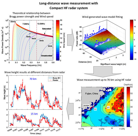
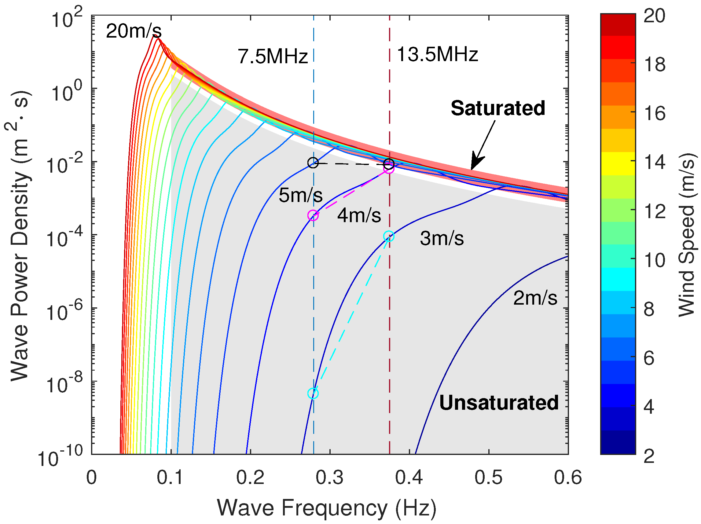
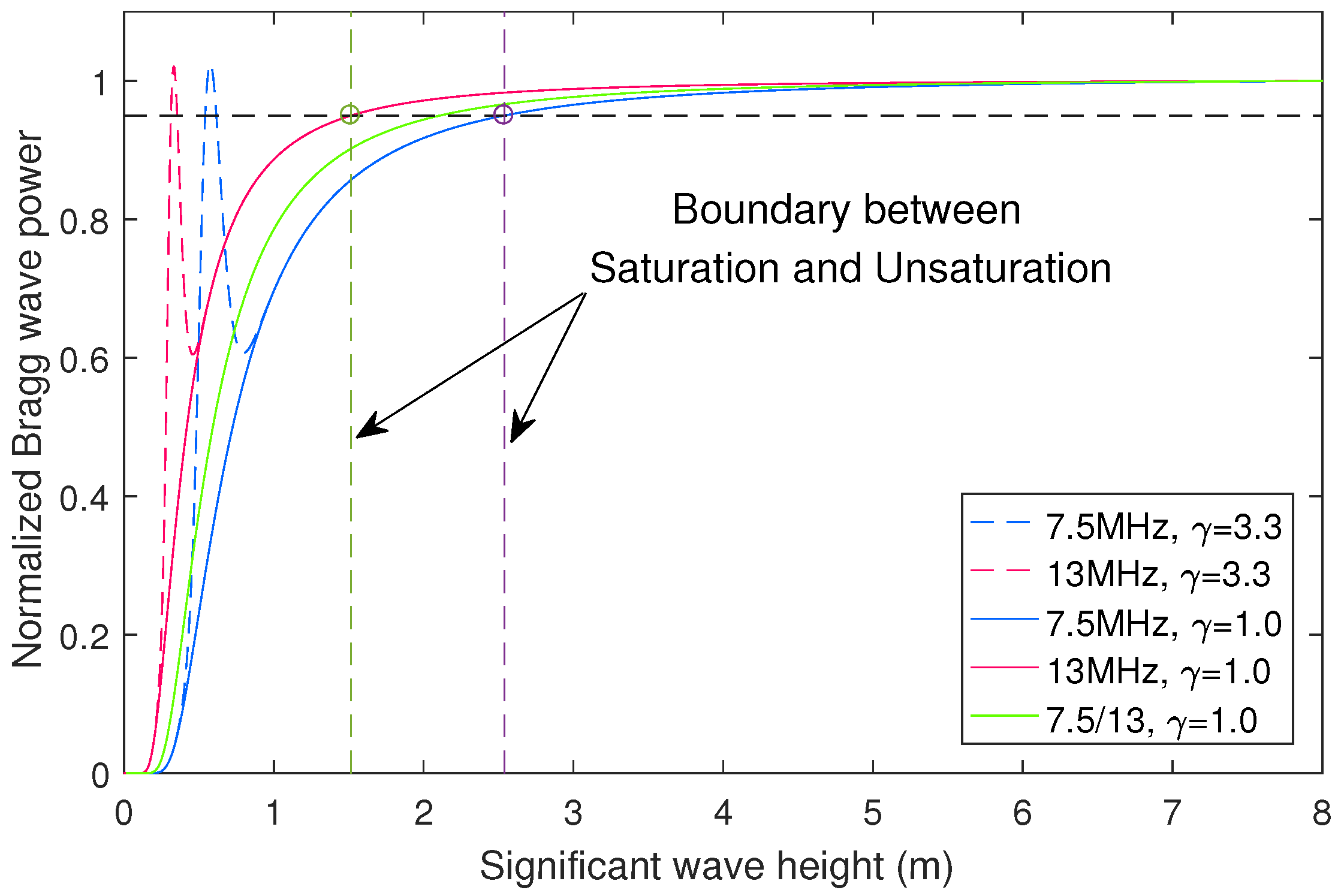
2.1. Relationship between First-order Echo Power and Wave Height

Among the different ground wave radar equations presented in previous literature [13,14,15,16], a synthesized formulation for monostatic HFSWR is adopted to express the received power backscattered from a sea surface patch locating at a distance of R from radar and in the direction of θ , with an area of Δ A = R Δ R Δ θ , where Δ R and Δ θ are the radar range and azimuth resolution, respectively.
P r ( R , θ ) = P t G t G r L m · 4 π λ 2 · σ s e a ( 1 ) · Δ A ( L b L a ) 2
P t is the average transmitted power, G t and G r are transmit and receive antenna gains, and L m is the miscellaneous system loss. λ is radar wavelength. L b is the one-way basic transmission loss associated with the radio propagation over smooth conducting sea plane, and L a is the additional propagation attenuation caused by the rough sea due to wind waves [17]. σ s e a ( 1 ) is the first-order scattering radar cross section (RCS). According to Barrick’s definition [17], L b is ( 2 π R / λ ) 2 . The attenuation caused by the coupling of antenna and its image in the ground, which was illustrated in [13,16], is a constant decided by the antenna height and is excluded here for simplification.
For a given radar frequency, Equation (1) can be simplified as
P r ( R , θ ) = Γ · Δ A L b 2 · σ s e a ( 1 ) L a 2 = Γ · 1 R 3 · σ s e a ( 1 ) L a 2
where Γ is a constant referring to the first two product terms on the right side of Equation (1), and Γ is the combination of Γ with the constants in Δ A and L b . The first-order RCS has been derived by Barrick as [1]
σ s e a ( 1 ) = 2 6 π k 0 4 m = ± 1 S 2 m k 0 · δ ω m ω B
where k 0 is the radar wavenumber, ω B = 2 g k 0 is the Doppler frequency of the resonant ocean wave. S ( · ) is the directional wave spectrum, which is the product of non-directional wave spectrum s ( ω ) and directional factor g ( θ + ϕ ) , ϕ is the wind direction with respect to the radar beam. The Bragg resonant condition is imposed by the delta-function δ ( · ) , indicating that the first-order RCS is actually proportional to the value of ocean wave spectrum at ω = ω B , as shown in Figure 1 (the samples are marked by the colored circles).
The first-order echo power P r ( R , θ ) is related to the significant wave height h s via wave spectrum S ( ω , θ + ϕ ) , since h s can be calculated as the integral of S ( ω , θ + ϕ + ψ ) over azimuth 0 ψ 2 π
h s = 4 S ( ω , ψ ) d ω d ψ = 4 S ( k , ψ ) k d k d ψ
It is worth noting that Equation (4) contains the contribution of all kinds of waves, including wind wave, swell wave and so on. The widely known ocean wave models such as JONSWAP spectrum [18], P-M spectrum [19] and Phillips spectrum [20], are all related to wind wave, and are defined as functions of the wind speed U. For swell and other waves, no special model is applicable. In many papers, such as [21,22], it has been pointed out that the first-order Bragg peaks at HF are produced by waves that respond quickly to the wind, viz. wind-generated waves. In other words, the first-order scattering is mainly associated with wind waves. Moreover, the first-order peaks have been used for wind direction estimation. For simplicity, only wind wave will be discussed in this paper. The widely applied wave model of JONSWAP spectrum is employed here, which can represent the fetch-limited sea state that is not fully-developed. The spectral density of this model is given by [18]
s ( ω ) = α g 2 ω 5 exp 5 4 ω p ω 4 γ exp ( ω ω p ) 2 2 σ 2 ω p 2
where
α = 0.076 U 10 2 g F 0.22
ω p = 22 g 2 U 10 F 1 / 3
σ = 0.07 ω ω p 0.09 ω > ω p
ω p is the peak wave frequency, g is the gravitational acceleration, U 10 is the wind speed at a height of 10 m above sea surface, F is the fetch length, and γ is the peak enhancement factor with the default value being 3.3. Inserting Equation (5) into Equation (4) obtains [18,23]
h s = 4 1.67 × 10 7 U 10 2 F g
A nondimensional fetch x ¯ = g F / U 10 2 is commonly used to illustrate the characteristics of the JONSWAP spectrum. It is concluded in [18] that, for large fetches x ¯ > 10 3 , the growth of the spectrum at low frequencies is governed by the wind forces rather than the wave-wave interactions, which results in a much flat peak and a reducing γ . Furthermore, a fetch x ¯ close to 10 5 indicates that the JONSWAP and P-M spectra are nearly identical and γ 1.0 . According to the relationship between significant wave height and wind speed examined by the buoys data collected at Taiwan Strait, we find that the resulted fetch x ¯ is around 10 4 .
Figure 1 shows the JONSWAP wave spectra under different wind speeds with x ¯ = 10 4 . The Bragg wave frequencies corresponding to two radar frequencies are marked by vertical dashed lines, and the crossed points marked by circles indicate the power of Bragg waves, which increases with wind speed till getting saturated at a certain level. The variations of Bragg wave power s ( ω B ) , normalized by its maximum value, with respect to significant wave height for the two frequencies are illustrated in Figure 2. The results obtained using the default value γ = 3.3 (dotted curves) and large fetch associated γ = 1.0 (solid curves) are compared. It is found that there is a sharp peak in the spectra obtained with γ = 3.3 , and the peak location, viz. ω p , equals to the radar Bragg frequency. However, in reality this spectral peak is rarely seen (see [9,11]). Hence, the influence of γ will not be discussed in this paper. If the saturation threshold value is set at 95%, a boundary between saturation and unsaturation is obtained, which has also been marked in Figure 1. The unsaturated region can be used to retrieve wave height from first-order backscatter. Different radar frequencies generate a different increasing slope due to the Bragg frequencies difference, thereby, the power ratio of the two frequencies (green solid curve) also increase with the wave height.

2.2. Model of Dual-Frequency Power Ratio with Wave height and Distance

The Bragg wave power s ( ω B ) , embedded in the first-order RCS σ s e a ( 1 ) , has been related to wave height theoretically (see Figure 2). It can be seen from Equations (2) and (3) that, there are still terms depending on location ( R , θ ) to be calibrated for modeling the relationship between P r ( R , θ ) and h s . These terms include g ( θ + ϕ ) and L a . The directional spreading of wave spectra changes with sea state [24], which results in different value of g ( θ + ϕ ) for different radar beam direction θ and wind direction. Hence, to model the dependence on direction θ , adequate information of wave height and wind speed over a wide angle coverage is necessary, which is hard to achieve. Note that g ( θ + ϕ ) is approximately the same between the two frequencies, so we can calibrate it easily by calculating the power ratio
η = P r 1 ( R , θ ) P r 2 ( R , θ ) = Γ r · s ( ω B 1 ) s ( ω B 2 ) · L a 2 ( f 2 ) L a 2 ( f 1 )
The residual constant of σ s e a ( 1 ) ( ω B 1 ) / σ s e a ( 1 ) ( ω B 2 ) , together with Γ 1 / Γ 2 , are rewritten as Γ r . The second term on the right hand side of Equation (10), i.e., the ratio of wave spectral values for two Bragg wave frequencies, increases with wave height because the Bragg wave corresponding to a higher frequency is easier to get saturated as wave height increases (see Figure 1). Taking JONSWAP spectrum for example and ignoring the γ involved term, the ratio s ( ω B 1 ) / s ( ω B 2 ) can be described as
s ( ω B 1 ) s ( ω B 2 ) = ω B 2 ω B 1 5 · exp 5 · 22 4 4 1 x ¯ 4 3 g U 10 4 1 ω B 1 4 1 ω B 2 4
Inserting Equation (9) into Equation (11), we find that the ratio is related to wave height with an exponential form. Hence, the following exponential model is employed, where a, b and c are three model coefficients introduced to account for possible uncertainties of the constant variables in Equations (9) and (11).
10 · log 10 s ( ω B 1 ) s ( ω B 2 ) = a + b · h s c
It is much more complex to model the additional propagation attenuation L a . The ratio, L a ( f 1 ) / L a ( f 2 ) , has been confirmed as a function of both distance R and wave height h s , but no exact model has been given in previous literatures. An assumption is made based on Barrick’s work [17] that a polynomial model of degrees less than or equal to 2 in R together with an exponential model of h s is feasible
10 · log 10 L a 2 ( f 2 ) L a 2 ( f 1 ) = ( d + e R + f R 2 ) · h s g
where d, e, f and g are extra model coefficients. Actually, this model is developed based on the simulated curve sets presented in [17]. Inserting Equations (12) and (13) into Equation (10), we get a model relating power ratio η to R and h s as
10 · log 10 η = a + b · h s c + ( d + e R + f R 2 ) · h s g
It is not easy to solve this equation to obtain h s for a given η and R. Nevertheless, a preliminary examination of this equation with experimental data shows that c g . Hence, the above model can be equally simplified as
10 · log 10 η = a + ( b + c R + d R 2 ) · h s e
From Equation (15), it is easy to derive the formula for calculating wave height as Equation (16). In addition, the maximum degree 2 of R suggests that three buoys at different distances are essential to provide wave height data for fitting.
h s = 10 · log 10 η a b + c R + d R 2 1 e
As we know, the first-order Bragg power varies with the distance and radar look direction in addition to the wave height. If we want to estimate wave height from Bragg power of a single radar frequency, a prior training over different distance and direction should be conducted. That is to say, wave height estimation at each location of the radar coverage is accompanied by an individual training. However, from the above analysis, it is concluded that the proposed dual-frequency based wave height estimation method mitigates the effect of direction, and requires a prior fitting with only three buoys at different distances. Hence, the training data required for the dual-frequency method can be significantly reduced.

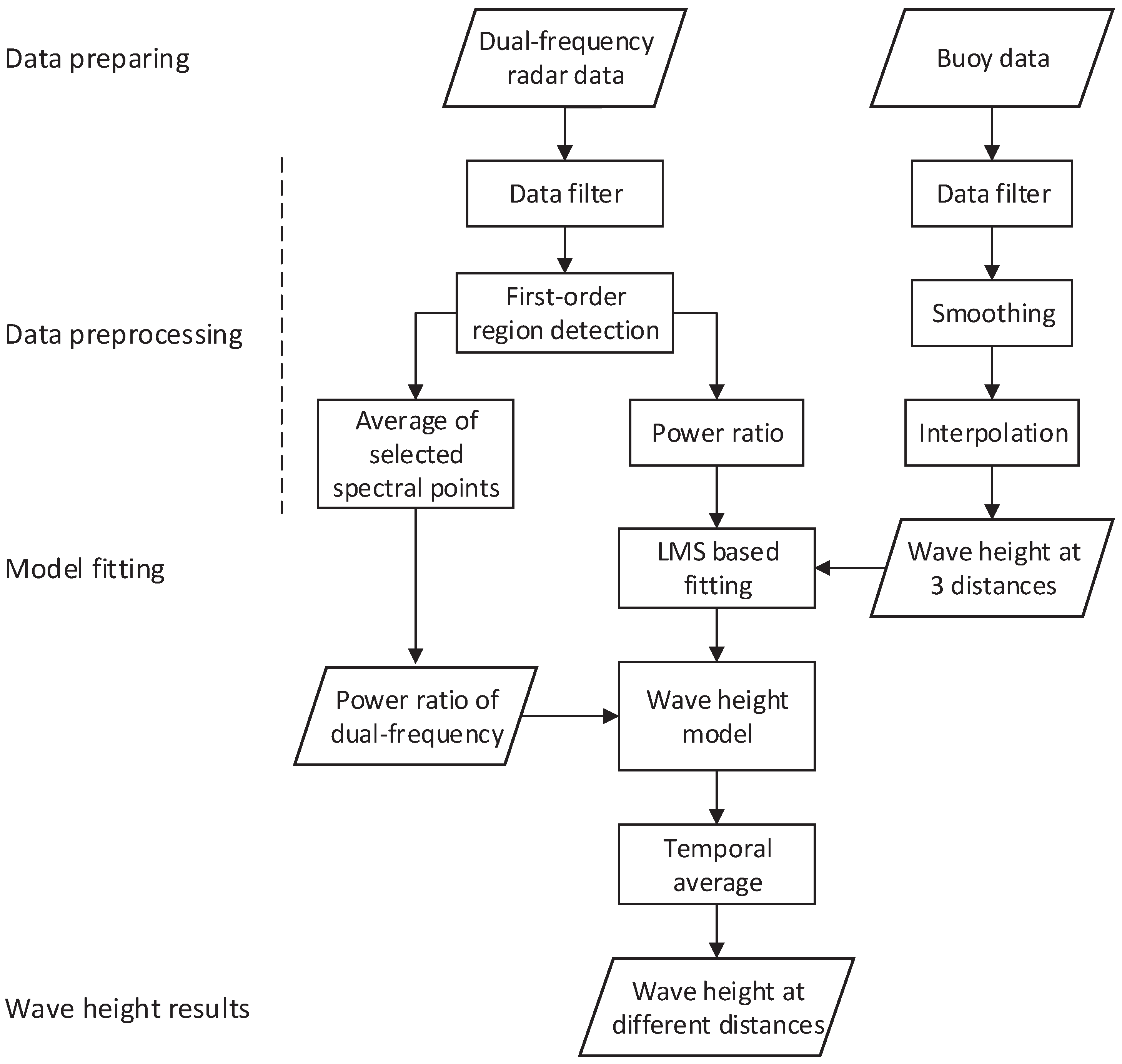
2.3. Block Diagram of the Wave Height Estimation

The overall procedure of the wave height estimation algorithm using dual-frequency radar data is illustrated in Figure 3. The critical step is to establish the relationship model among power ratio, wave height and distance through fitting the radar data to in situ buoy data. The fitting error determines the final wave height estimation error. Hence, a proper selection of fitting data is necessary and important. For Buoy data, the invalid and incorrect data should be identified and excluded, followed by a subsequent temporal smoothing and interpolation, to minimize the data error. As for radar data, those with dense radio frequency interference should be detected and removed. Subsequently, the stronger Bragg peak located on the same side (positive or negative) of the Doppler spectra obtained by the radar at two frequencies is detected. From the detected Bragg region, the spectral points within 5 dB (a empirical value proved to be valid) lower than the peak point are selected, which are supposed to be resulted from directions with fairly uniform wave field. The following processing is slightly different between model fitting and wave height estimation. Model fitting concentrates on the overall scatter relationship between Bragg power ratio and wave height, therefore, the selected spectral points are directly taken into account. The model coefficients, ( a , b , c , d , e ) in Equation (15), are calculated through Least mean square (LMS) fitting. However, for wave height estimation, spatial average and median filtering are required to reduce the fluctuation of η . Finally, we can estimate the wave height results over different distances according to Equation (16). Temporal average is also necessary to control the data quality.

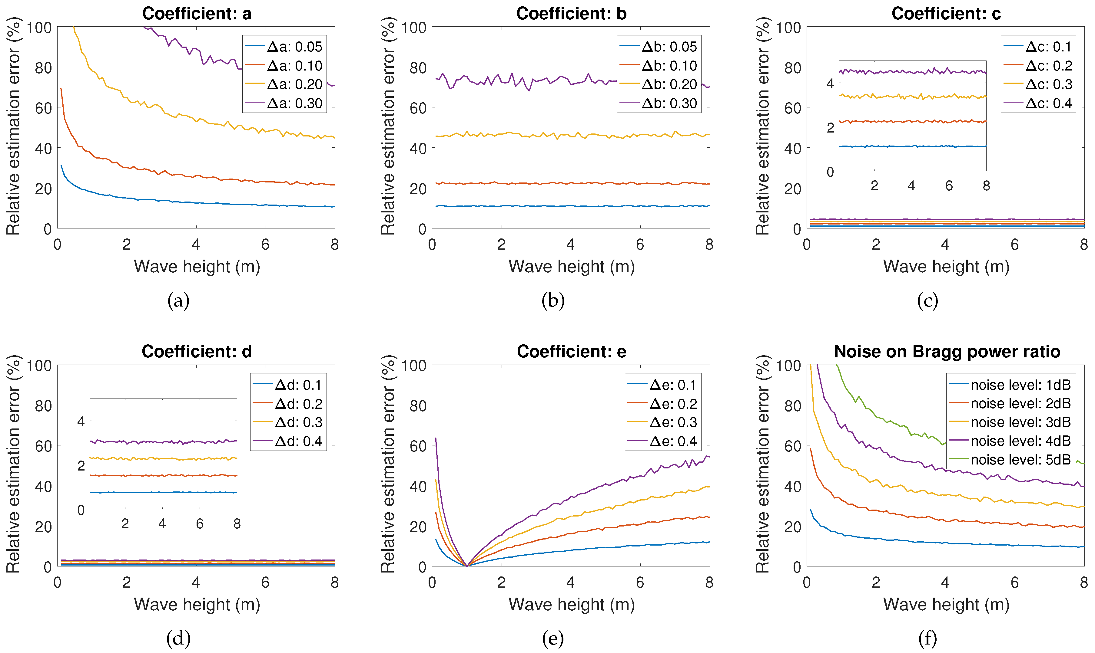
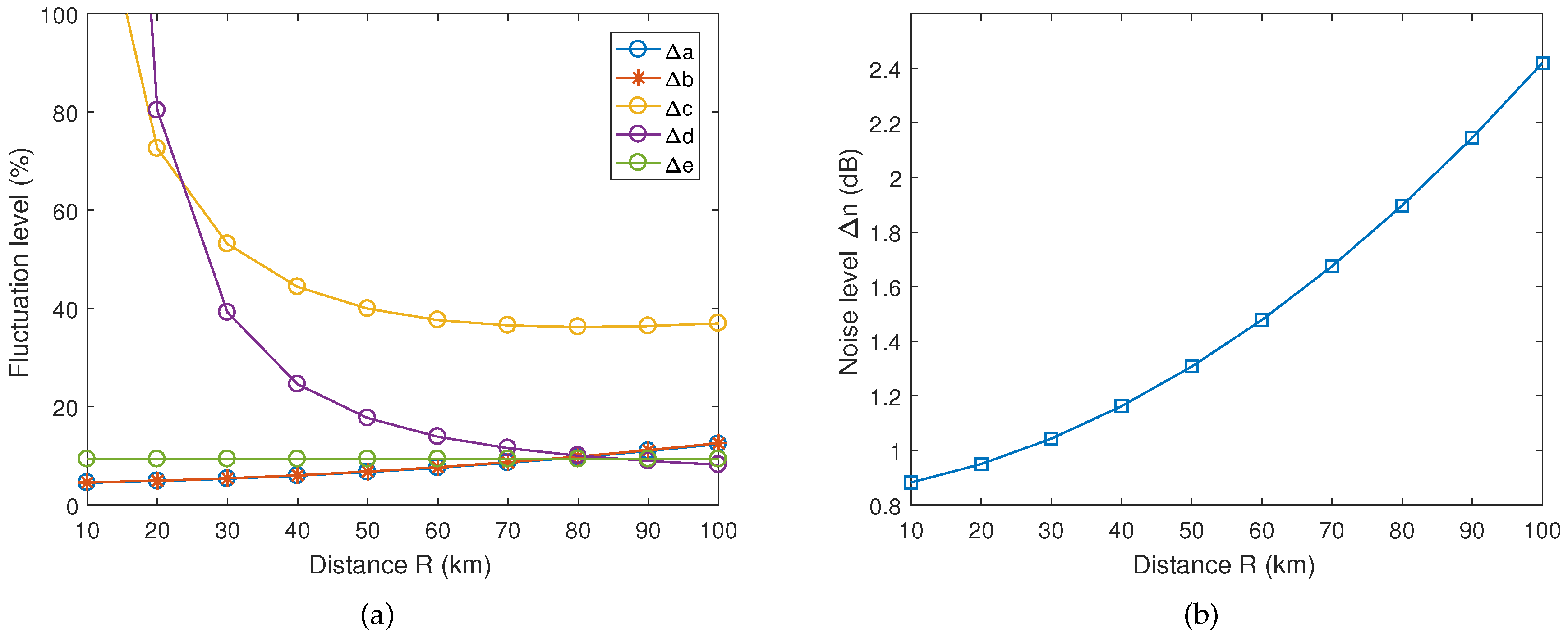
3. Numerical Analysis

A numerical analysis based on simulation is carried out to examine the robustness of the wave height estimation algorithm, by evaluating the relation of wave height estimation error with respect to the noise effect on the Bragg power ratio and the inaccuracy in the fitting coefficients, viz. a, b, c, d and e. The fitting coefficients depend on experiment parameters such as the radar system configuration and properties of the observed ocean area, e.g. seawater salinity. A set of empirical values, a = 22.12 , b = 13.76 , c = 0.047 , d = 0.0021 , e = 0.241 , determined from the field experiment data (see Section 4.2.2) are applied for simulation.
For a given wave height h s , a corresponding ratio η can be obtained from Equation (15). The noise is added by replacing 10   log 10 η with 10   log 10 η + Δ n · n ( t ) , t = 1 , 2 , , L , where n ( t ) U ( 1 , 1 ) is a uniformly distributed random variable with a value within 1 to + 1 . Δ n is the noise level in decibels, and the number of independent trials L is 300. The estimated wave height h s using Equation (16) deviates from the true value h s in presence of n ( t ) , and the error Δ h s = | h s h s | relies on the noise level Δ n . The possible uncertainties of coefficients generated in applying LMS fitting to the noise-contaminated data are represented by the additive fluctuation, taking coefficient a for example, a + a · Δ a · n ( t ) denotes the fluctuated form with Δ a being the fluctuation level in percentage. The dependence of wave height estimation error on noise and fluctuation of each coefficient are studied individually for different sea states, as shown in Figure 4 in which the distance R is set as 15 km. Here, the relative error (the ratio of absolute error | h s h s | to wave height h s ) is used, and the root mean square difference is calculated under each wave height condition in terms of L independent trials.
Figure 4(a–e) shows that the wave height estimation is much more sensitive to the fluctuation of coefficients a, b and e, but almost not influenced by c and d. The effect of noise is also remarkable that a change of Bragg power ratio within ± 5 dB can lead to a relative estimation error up to 60%. Moreover, an increasing relative error with a decrease in wave height is observed for the cases associated with coefficient a, e and noise, nevertheless, the corresponding absolute error is not too large. If the wave height estimation error is limited to h s · 10 % + 0.5 m , a moderate value decided according to the specifications of SeaSonde [25] for which the typical wave height accuracy is 7–15% (adding 0.5 m to deal with low sea state cases), the corresponding acceptable fluctuation levels for ratio η and coefficients a, b, e are Δ n < 1 dB, Δ a < 0.05 , Δ b < 0.05 and Δ e < 0.1 , respectively. Furthermore, the acceptable fluctuation levels change with distance (see Figure 5). An increased distance results in a much more relaxed limitations on noise level and fluctuation of coefficients a, b and e. However, this is not true for coefficients c and d since they are directly related to distance R according to Equation (16).

4. Experimental Results

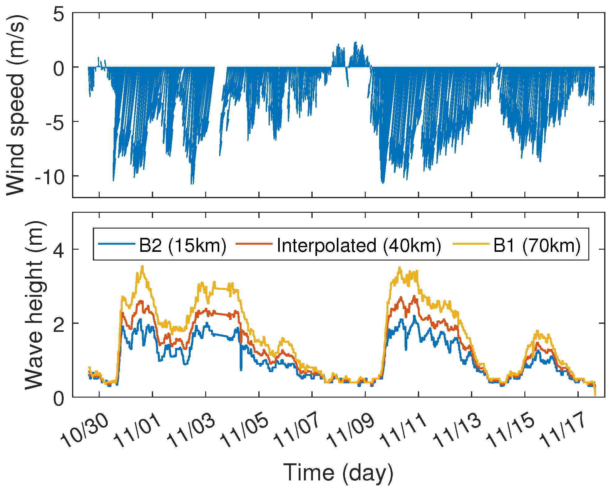
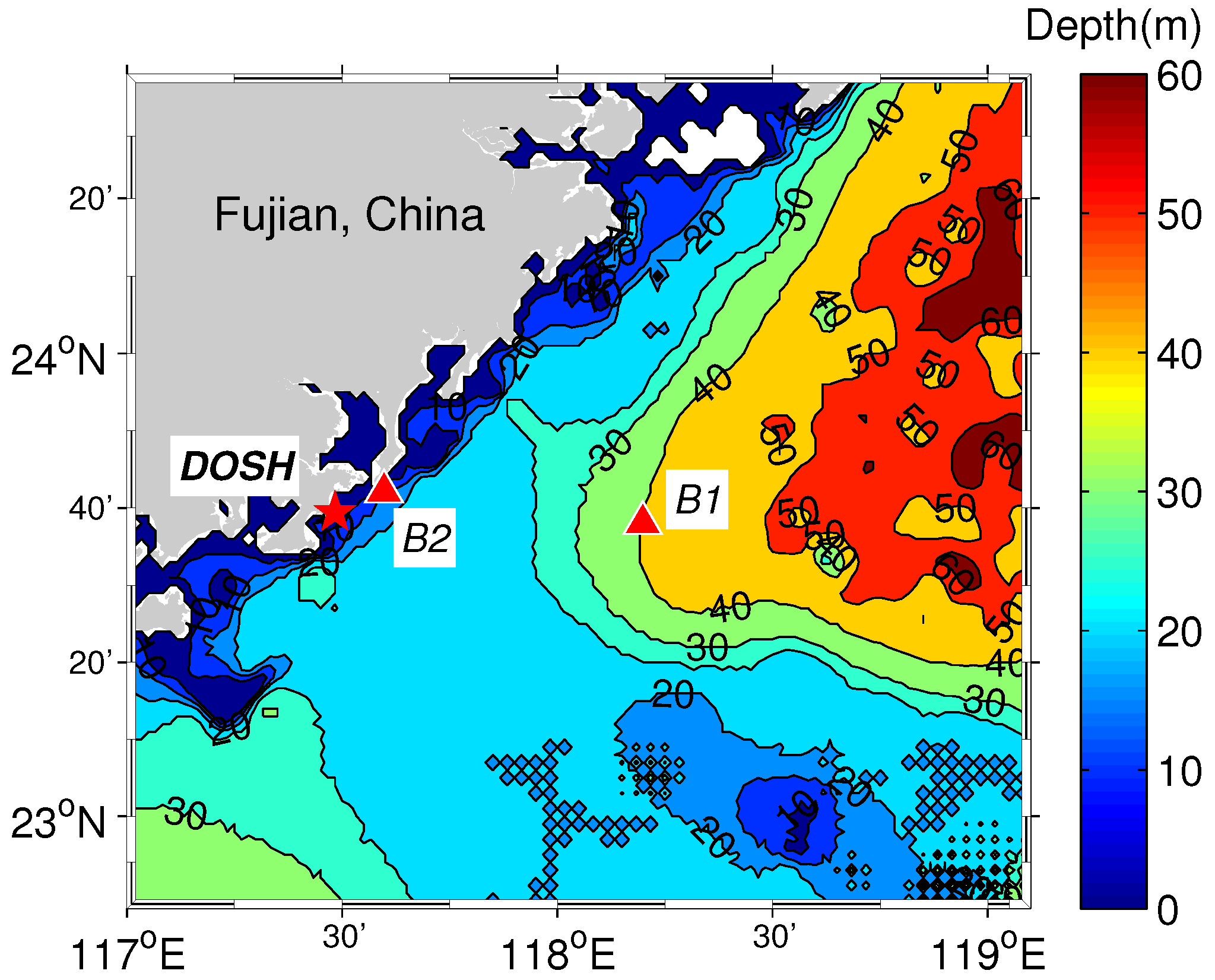
4.1. Experiment Data Description

To validate the proposed method, a 20-day experiment was conducted on the coast of Taiwan Strait from October to November in 2015 (see Figure 6). The radar was deployed at Dongshan (abbreviated as DOSH), a small village in Fujian province of China. Two in situ buoys were available for providing concurrent wave height data. The water depth distribution is also plotted.
The radar (OSMAR-SD) used here was developed by the Radar and Signal Processing Laboratory (RSPL) at Wuhan University and it consists of a dual-frequency, fully-digital transceiver and compact antennas [12,26]. The fully-digital structure can be flexibly configured to work at single- or dual-frequency. At the dual-frequency mode, the two frequencies are swept and de-chirped alternatively by sweep period to ensure the simultaneity. Like SeaSonde [27], monopole and crossed-loop antennas are, respectively, used for transmitting and receiving. However, both of the transmit and receive antenna have been redesigned to be able to work at dual-frequency at the meantime without changing their appearance. More details about the dual-frequency crossed-loop antenna can be found in [28]. The main system characteristics configured for this experiment are listed in Table 1. The coherent integration time (CIT) which is set as 553 s for both frequencies, is close to the time-resolution of the buoy data, 10 minutes.
The wind and wave height data collected from in situ buoys during the experiment period are depicted in Figure 7. Wind data from only one buoy is plotted due to the similarity of both. The wave height data of two buoys, B1 and B2, are strongly correlated. Note that at least three buoys located at different distances are required for the fitting of the model in Equation (15). By considering the scalable difference caused by the water depth, it is reasonable to obtain the wave height at the middle distance (i.e., 40 km) via interpolation. Another interesting phenomenon noticed from the wind data is that the wind always blows from northeast to southwest during the whole experiment period. This seasonal phenomenon is unique due to the special geographic feature of Taiwan Strait.

4.2. Results of Model Fitting and Wave Height Estimation

Two steps are involved in establishing the relationship between power ratio η and wave height h s . First, it is necessary to investigate whether the ratio of Bragg wave power varies with wave height according to a specific model. Second, the R and h s dependent term associated with additional propagation attenuation should be calibrated.

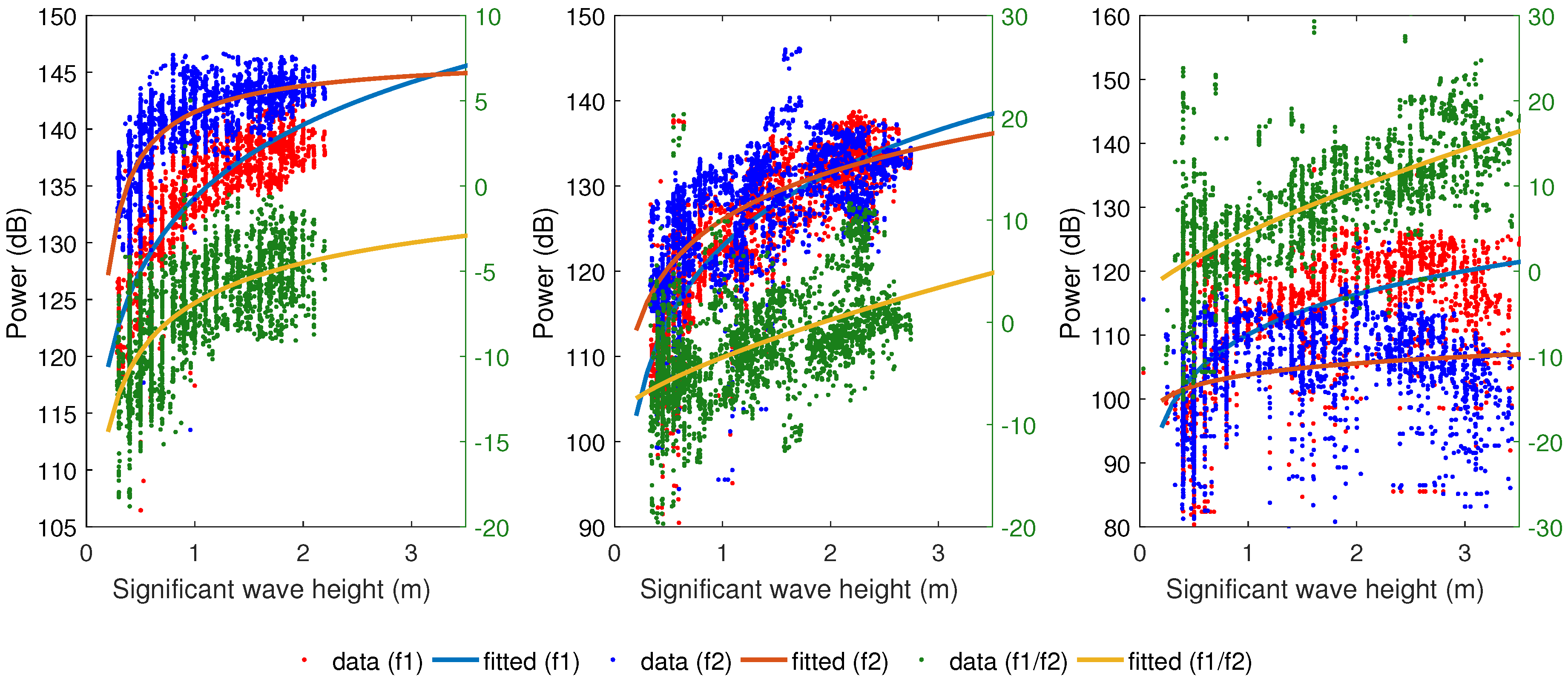
4.2.1. Two-dimensional fitting: Bragg power and h s

The overall variations of the Bragg echo level are examined with respect to wave height. Figure 8 illustrates this at three different distances. Both the results of single frequency (red dots: f 1 , blue dots: f 2 ) and ratio of dual-frequency (green dots) are plotted, and the solid lines represent the fitted curves. The model presented in Equation (12) is used for fitting in both single- and dual-frequency cases. When applied for single frequency fitting, the power ratio on the left side of Equation (12) is alternatively replaced by the first-order echo power of single frequency. The corresponding fitted coefficients and errors are listed in Table 2. It can be seen that the fitting results worsen with the distance, due to the decline of signal-to-noise ratio (SNR). Note that sea clutter is dominated by the Bragg wave power s ( ω B ) at a near range (e.g. 15 km) since additional propagation attenuation L a is negligible. It is found that the Bragg wave power ratio of dual-frequency does vary with h s , and the fitting correlation coefficient is 0.70.

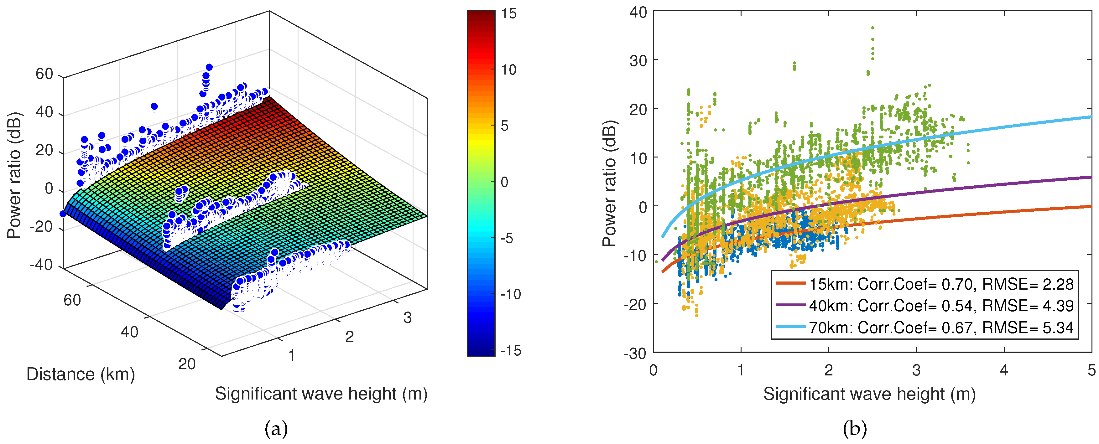
4.2.2. Three-dimensional fitting: Bragg power ratio and ( h s , R )

The second step is to conduct the three-dimensional fitting with respect to h s and R, using the model given in Equation (15). The fitting result is shown in Figure 9a, and the fitting coefficients as well as the confidence bound are listed in Table 3. The fitting coefficient values used for wave height estimation is determined by the mean value of the 95% confidence bound. The absolute uncertainty of the fitting coefficients is defined by the bias between the confidence bounds and the mean values, and the relative uncertainty is obtained by the ratio of absolute uncertainty to the mean value. A higher ratio implies a lower dependence of the fitting model upon the associated coefficient, and vice versa. The fitting errors in wave height estimation, noted in Figure 9b, are very close to that obtained using 2-dimensional fitting (see Table 2). This verifies the validity of the polynomial model.

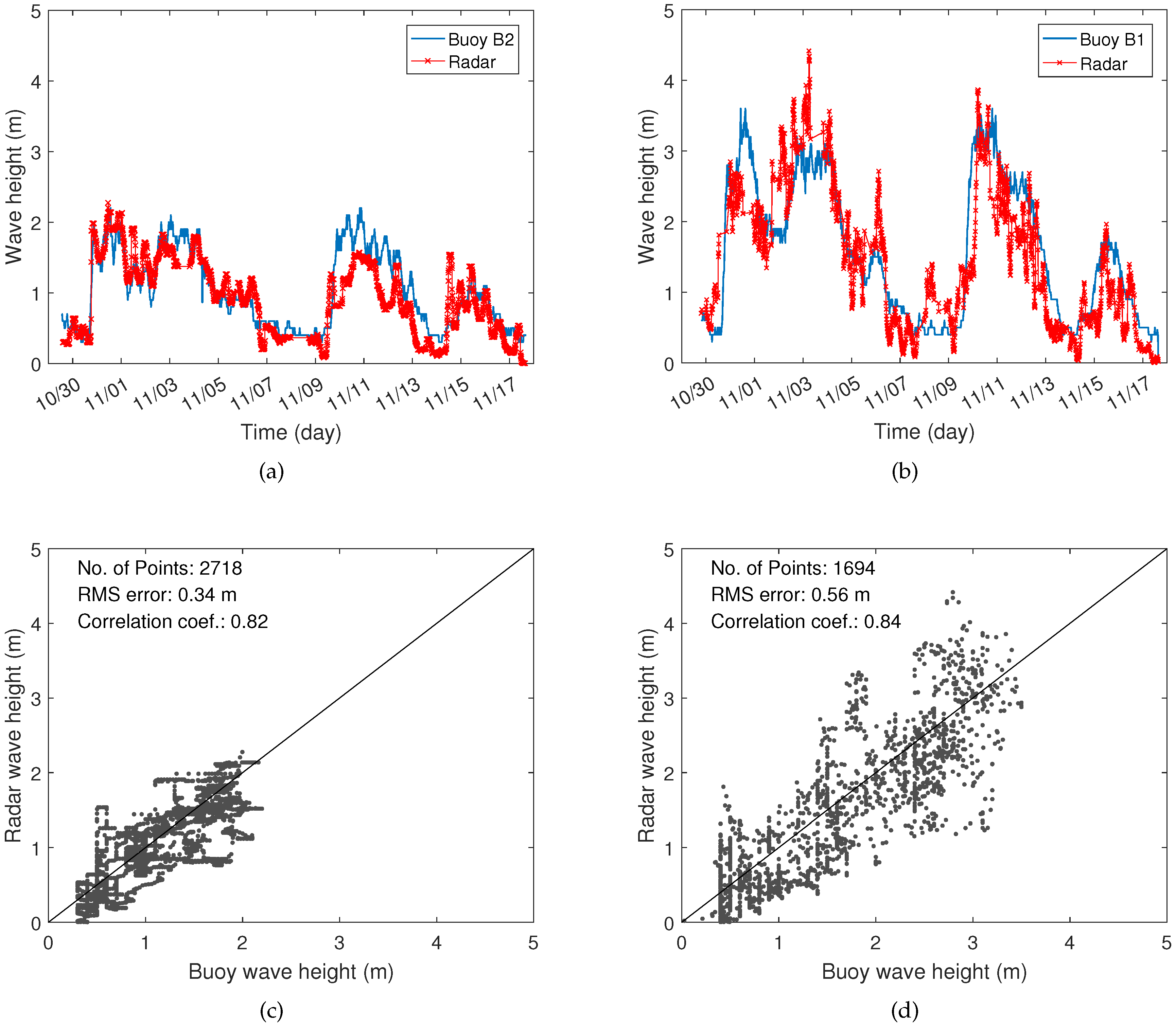
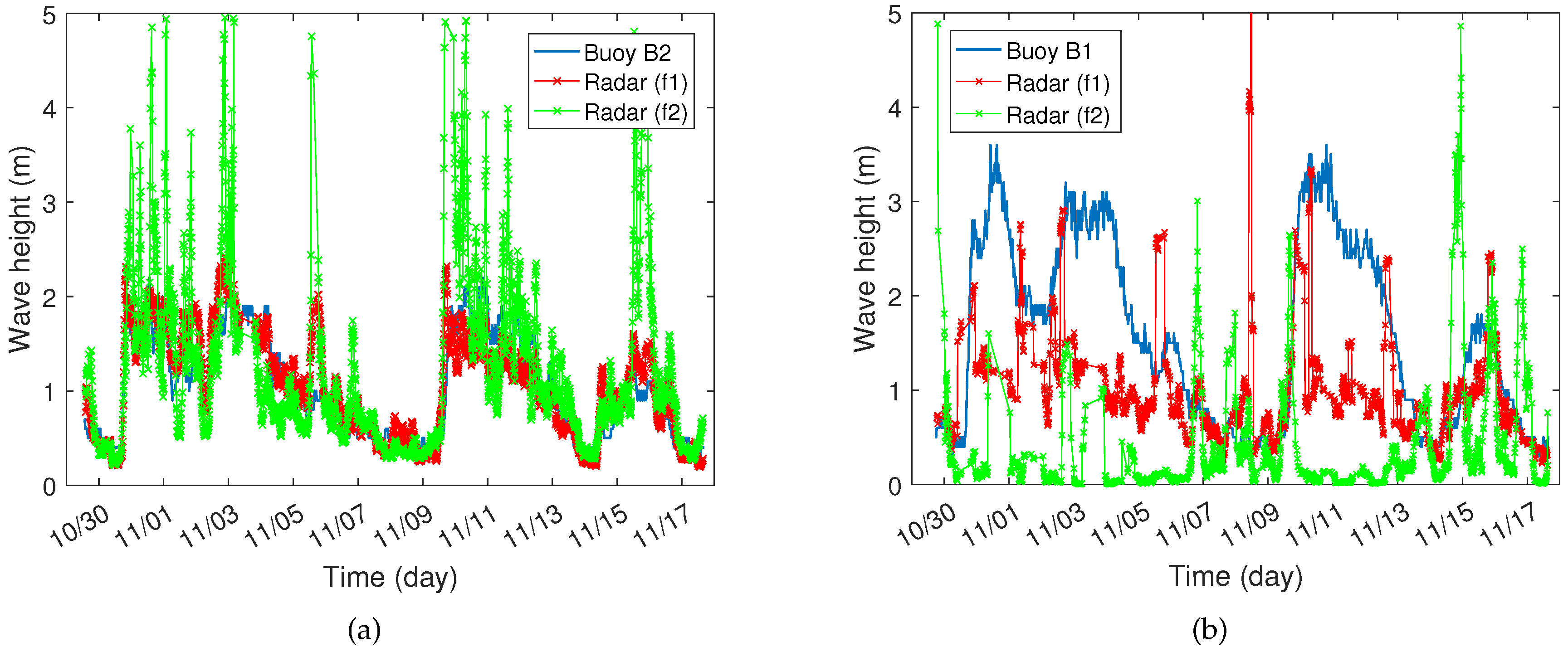
4.2.3. Wave Height Estimation Results

The wave height results for the whole dataset are obtained according to Equation (16) with the fitted coefficients, as depicted in Figure 10. The wave height measured by the radar (red dots) agrees well with the buoy data (blue lines) collected at 15 km and 70 km. The associated root mean square error (RMSE) are 0.34 m and 0.56 m with correlation coefficients of 0.82 and 0.84, respectively.
As a comparison, wave height results estimated from the first-order Bragg power of the two single frequencies independently by inverting Equation (12) and applying the fitting coefficients illustrated in Section 4.2.1, are also given in Figure 11. Table 4 lists the statistic results of both single-frequency and dual-frequency comparisons.

5. Discussion

From Figure 8 and Table 2, it is observed that the fitting results of single frequency f 1 and f 2 are better than that of dual-frequency at 15 km with higher correlation coefficients. The subsequent wave height estimation results, presented in Figure 10, Figure 11 and Table 4, also show that the single frequency based method, particularly using f 1 , seems to obtain a comparable result with that of the dual-frequency. Nevertheless, it is just a coincidence due to the stationary wind direction in this special area, and the effect of wind direction is negligible here. If the directional spreading calibration is required, dual-frequency deployment would be preferred. Moreover, single-frequency based method is limited to both the nearshore and low sea state conditions in order to mitigate effect of additional propagation attenuation. It can be seen from the results obtained at 70 km that, the wave height results estimated using two single frequencies independently are much worse than that with the dual frequency. Because the first-order spectral power for single frequency system is more susceptible to additional propagation attenuation with increased wave height and distance, but the Bragg peak power ratio of a dual-frequency radar is not significantly affected. Besides, an unexpected decline in the correlation of dual-frequency case at 40 km is found to be caused by target interference that appeared inside the Bragg region, while the interference locations are different between the two operating frequencies.
By observing Figure 10, it may be seen that several fast-changing periods occurring at 15 km, e.g. around October 31, are identified successfully. The overall estimation at 15 km is superior to that at 70 km due to a higher echo SNR, except for the underestimation of two segments around November 10 and 12. The reason for the underestimation is due to the significantly spread Doppler spectrum caused by a strong current velocity. In the coastal region, the water depth changes rapidly with azimuth even at a same distance from radar, and wave height also differs significantly. Hence, backscatter averaged over a broad azimuthal range will lead to a less precise estimation. However, it will be much better in a case of low current velocity when the strongest spectral points are mainly arisen from a narrower beamwidth. Furthermore, the setting of the SNR threshold in selecting the spectral points and other unwanted signals appearing in the Bragg clutter will also affect the estimation result.
The 3-dimensional fitting results presented in Figure 9 and Table 3 show that the proposed wave height model has different degree of dependence on different coefficients, e.g., coefficient c contributes the least influence, which has also been revealed in the numerical analysis in Section 3. According to the conclusion drawn by simulation, the acceptable error in fitting coefficients required to achieve desirable wave height estimation accuracy varies at different distances. It seems that the fitting confidence bounds do not satisfy the theoretical constraints over all of the radar coverage, i.e 10∼100 km. However, it is worth mentioning that the numerical analysis of the effects was conducted for each coefficient separately. While, for the field data , the uncertainties of all the coefficients are considered together. The overall influence of multi-coefficient fluctuations is extremely different from that of a single one because the effects caused by different parameters compensate, which is eventually equivalent to what results from noise on power ratio. It is seen from Figure 9b that the fitting RMSEs increase with distances, i.e. 2.28 dB at 15 km and 5.34 dB at 70 km, which are both larger than the values required by the simulation, i.e. 0.9 dB at 15 km and 1.7 dB at 70 km (see Figure 5b). The larger noise level at 70 km leads to worse wave height estimation. However, an acceptable wave height result is obtained at 15 km. This looks contradicting the simulation conclusion. The possible reason is that the data used for fitting accounts for all the spectral points in the identified Bragg region without spatial averaging and time averaging, as a consequence, the fluctuations are relatively large. However, in real wave height estimation, both spatial and time averaging are employed in advance so that the fluctuation of Bragg power ratio has been significantly reduced, therefore, desirable wave height results are obtained, implying that the algorithm is robust and applicable.
It also should be noted that, 1) the fitting model is proposed based on the JONSWAP spectrum, but the difference due to using different wave spectrum models is embedded in the power term in Equation (12). Hence, the final fitting and wave height estimation are not limited to the selected model. Besides, no false solution occurs in the fitting. 2) Although for fully-developed sea that wave height can be directly calculated from wind speed, the proposed method is based on the fitting between the Bragg power ratio and wave height, and it does not require any wind speed data. Hence, in the case of developing or swell-contaminated sea, wave height can also be estimated, but wind speed may not.

6. Conclusion

In this paper, an improved wave height estimation method using first-order Bragg backscatter of a dual-frequency radar is presented. A theoretical relationship between wave height and the ratio of first-order echo power associated with two frequencies is derived based on the radar equation and wave spectra model. This ratio actually reflects the different speed of Bragg wave growing with sea state for two frequencies. Compared with the measurement using single frequency radar, employing a dual-frequency radar has an advantage in calibrating the distance and direction dependent uncertainty within the radar equation so that wave height can be estimated at different distances, and potentially, over different directions. Preliminary investigation of the relationship among Bragg peak power ratio of a dual-frequency radar system and distance, wave height has been conducted based on a 20-day field data. Fitting the radar data to in situ buoy data over different distances shows that a polynomial model of degree 2 in distance and degree less than 1 in wave height works well. Subsequent comparison of wave height measured by radar and buoy at distances of 15 km and 70 km demonstrates the validity of this method. A RMSE of 0.34 m and 0.56 m and correlation coefficient of 0.82 and 0.84, respectively, are obtained.
However, spike-like fluctuations are still seen in wave height results even after performing both temporal and directional average and median smoothing. This is supposed to be the result of combining all Bragg spectral points selected together. Thus, a better scheme for selecting Bragg spectral points should be further investigated in the future. In addition, ongoing work also includes the comparison and validation of direction dependency calibration in case of varying wind direction by using single- and dual-frequency data, as well as the separation of wave height over different directions, i.e. obtaining the wave field. Besides, the experiment site selected in this paper is special for its local subtropical monsoon climate. The wind mainly blows along the strait, i.e. along the shore, which results in a wave spectrum corresponding to a large fetch. Hence, the sea under investigation can be treated as fully developed. Nevertheless, investigation of the performance of the proposed method over pure fetch-limited sea should be conducted for the case with an offshore wind blowing perpendicular to the shore in the future. Furthermore, the discussion in this paper only considers sea state generated by wind blowing from single direction with single speed. The case that sea state at one location generated by winds blowing from different directions with different speeds and fetch lengths should also be included. Moreover, it is worth validating the proposed method with local wave model results in the future.

Acknowledgments

This work was supported in part by the Ocean Public Welfare Scientific Research Project under grant 201205032-3, in part by the National Special Program for Key Scientific Instrument and Equipment Development of China under grant 2013YQ160793, and in part by the Fundamental Research Funds for the Central Universities under grant 2042016kf0019. The authors are also grateful to Fujian Marine Forecasts, China, for providing the buoy data.

Author Contributions

Y. T. as the main author proposed the method, designed and conducted the experiments, performed the data processing and analysis, and wrote the manuscript. B. W. supervised and advised the research work that led to this paper. H. Z., C. W. and J. Y. reviewed the manuscript and contributed to discussions. W. H. contributed to discussions and revision of the writing.

Conflicts of Interest

The authors declare no conflict of interest.

References

  1. Barrick, D.E. First-order theory and analysis of MF/HF/VHF scatter from the sea. IEEE Trans. Antennas Propag. 1972, AP-20, 2–10. [Google Scholar] [CrossRef]
  2. Barrick, D.E. The ocean waveheight nondirectional spectrum from inversion of the HF sea-echo Doppler spectrum. Remote Sens. Environ. 1977, 6, 201–227. [Google Scholar] [CrossRef]
  3. Lipa, B.J.; Nyden, B. Directional wave information from the SeaSonde. IEEE J. Ocean. Eng. 2005, 30, 221–231. [Google Scholar] [CrossRef]
  4. Gurgel, K.W.; Essen, H.H.; Schlick, T. An Empirical Method to Derive Ocean Waves From Second-Order Bragg Scattering: Prospects and Limitations. IEEE J. Ocean. Eng. 2006, 31, 804–811. [Google Scholar] [CrossRef]
  5. Wyatt, L.R. Limits to the inversion of HF radar backscatter for ocean wave measurement. J. Atmos. Ocean. Technol. 2000, 17, 1651–1666. [Google Scholar] [CrossRef]
  6. Wyatt, L.R. Wave measurements from the Australian Coastal Ocean Radar Network. In Proceedings of the OCEANS 2014—TAIPEI, Taipei, Taiwan, 7–10 April 2014; pp. 1–5. [Google Scholar]
  7. Hisaki, Y. Development of HF radar inversion algorithm for spectrum estimation (HIAS). J. Geophys. Res. Oceans 2015, 120, 1725–1740. [Google Scholar] [CrossRef]
  8. Wyatt, L.R.; Liakhovetski, G.; Graber, H.C.; Haus, B.K. Factors Affecting the Accuracy of SHOWEX HF Radar Wave Measurements. J. Atmos. Ocean. Technol. 2005, 22, 847–859. [Google Scholar] [CrossRef]
  9. Shen, W.; Gurgel, K.W.; Voulgaris, G.; Schlick, T.; Stammer, D. Wind-speed inversion from HF radar first-order backscatter signal. Ocean Dyn. 2012, 62, 105–121. [Google Scholar] [CrossRef]
  10. Kirincich, A. Remote Sensing of the Surface Wind Field over the Coastal Ocean via Direct Calibration of HF Radar Backscatter Power. J. Atmos. Ocean. Technol. 2016, 33, 1377–1392. [Google Scholar] [CrossRef]
  11. Zhou, H.; Wen, B. Wave Height Extraction From the First-Order Bragg Peaks in High-Frequency Radars. IEEE Geosci. Remote Sens. Lett. 2015, 12, 2296–2300. [Google Scholar] [CrossRef]
  12. Tian, Y.; Wen, B.; Zhou, H. Measurement of High and Low Waves Using Dual-Frequency Broad-Beam HF Radar. IEEE Geosci. Remote Sens. Lett. 2014, 11, 1599–1603. [Google Scholar] [CrossRef]
  13. Milsom, J.D. HF Groundwave Radar Equations. In Proceedings of the Seventh International Conference on (Conf. Publ. No. 441) HF Radio Systems and Techniques, Nottingham, UK, 7–10 July 1997; pp. 285–290. [Google Scholar]
  14. Grosdidier, S.; Baussard, A.; Khenchaf, A. HFSW Radar Model: Simulation and Measurement. IEEE Trans. Geosci. Remote Sens. 2010, 48, 3539–3549. [Google Scholar] [CrossRef]
  15. Shearman, E.D.R. Propagation and scattering in MF/HF groundwave radar. IEE Proc. F Commun. Radar Signal Process. 1983, 130, 579–590. [Google Scholar] [CrossRef]
  16. Leong, H. On the Feasibility of Using Measured Sea Clutter Continuum In HFSWR to Validate Modelled Ground-Wave Propagation Attenuation in Rough Sea; Defence R&D Canada: Ottawa, ON, Canada, 2012. [Google Scholar]
  17. Barrick, D.E. Theory of HF and VHF Propagation Across the Rough Sea, part I & II. Radio Sci. 1971, 6, 517–533. [Google Scholar]
  18. Hasselmann, K.; Barnett, T.; Bouws, E.; Carlson, H.; Cartwright, D.; Enke, K.; Ewing, J.; Gienapp, H.; Hasselmann, D.; Kruseman, P.; et al. Measurements of wind wave growth and swell decay during the Joint North Sea Wave Project (JONSWAP). Dtsch. Hydrogr. Z 1973, 12, 1–95. [Google Scholar]
  19. Pierson, W.; Moskowitz, L. A proposed spectral form for fully developed wind seas based upon the similarity theory of S.A. Kitaigorodskii. J. Geophys. Res. 1964, 69, 5181–5190. [Google Scholar] [CrossRef]
  20. Phillips, O.M. The Dynamics of the Upper Ocean; Cambridge University Press: Cambridge, UK, 1966. [Google Scholar]
  21. Long, A.; Trizna, D. Mapping of North Atlantic winds by HF radar sea backscatter interpretation. IEEE Trans. Antennas Propag. 1973, 21, 680–685. [Google Scholar] [CrossRef]
  22. Lipa, B.J.; Barrick, D.E. Methods for the extraction of long-period ocean wave parameters from narrow beam HF radar sea echo. Radio Sci. 1980, 15, 843–853. [Google Scholar] [CrossRef]
  23. Naderi, M.; Pätzold, M. Design and analysis of a one-dimensional sea surface simulator using the sum-of-sinusoids principle. In Proceedings of the OCEANS 2015—MTS/IEEE Washington, Washington, DC, USA, 19–22 October 2015; pp. 1–7. [Google Scholar]
  24. Tyler, G.L.; Teague, C.C.; Stewart, R.H.; Peterson, A.M.; Munk, W.H.; Joy, J.W. Wave directional spectra from synthetic aperture observations of radio scatter. Deep Sea Res. 1974, 21, 989–1016. [Google Scholar] [CrossRef]
  25. Codar. SesSonde general specifications. Available online: http://www.codar.com/images/products/SeaSonde/1A-SeaSonde_v2_20100331.pdf. (accessed on 27 September 2017).
  26. Tian, Y.; Wen, B.; Tan, J.; Li, K.; Yan, Z.; Jing, Y. A new fully-digital HF radar system for oceanographical remote sensing. IEICE Electron. Express 2013, 10, 1–6. [Google Scholar] [CrossRef]
  27. Liu, Y.; Weisberg, R.H.; Merz, C.R. Assessment of CODAR SeaSonde and WERA HF Radars in Mapping Surface Currents on the West Florida Shelf. J. Atmos. Ocean. Technol. 2014, 31, 1363–1382. [Google Scholar] [CrossRef]
  28. Li, Z.; Wen, B.; Tian, Y. Design and Implementation of a Dual-Frequency Compact Antenna System for HF Radar. IEEE Antennas Wirel. Propag. Lett. 2017, 16, 1887–1890. [Google Scholar] [CrossRef]
Figure 1. Ocean wave non-directional spectra under different wind speeds (JONSWAP spectrum [18] is selected for example). The wave frequencies resonant to two radar frequencies (7.5 MHz and 13.5 MHz) are indicated by the location of the vertical dashed lines.
Remotesensing 09 01186 g001
Figure 2. Normalized Bragg wave power at different wave height. The horizontal dashed line represents the threshold value of 95% of maxima. The corresponding wave height boundaries are drawn by the vertical dashed lines.
Remotesensing 09 01186 g002
Figure 3. Block diagram of the wave height estimation algorithm.
Remotesensing 09 01186 g003
Figure 4. Effects of fluctuations of different fitting coefficients such as (a) a, (b) b, (c) c, (d) d and (e) e, and (f) noise added to the Bragg power ratio on the estimation of wave height.
Remotesensing 09 01186 g004
Figure 5. The limitations on (a) the error of the fitting coefficients and (b) the noise level on the power ratio, subject to the root mean square error of estimated wave height being within h s · 10 % + 0.5 m.
Remotesensing 09 01186 g005
Figure 6. Map of the experiment site over the Taiwan strait. The water depth is depicted in the form of filled bathymetric contour. The HF radar was deployed at the site of DOSH marked by red pentagram. There were two buoys marked as B1 and B2 with red triangles, which are, respectively, 73 km and 12.7 km away from the radar in the direction of 91.8° and 66.6° with respect to the north.
Remotesensing 09 01186 g006
Figure 7. Wind (top) and wave height (bottom) data of buoys. The wind data is collected by buoy B2, and the wave height at the distance of 40 km is obtained by interpolating the data from B1 and B2.
Remotesensing 09 01186 g007
Figure 8. Statistic relationship between wave height and Bragg echo power of single frequency and dual-frequency radar data at different distances: 15 km (left), 40 km (middle) and 70 km (right).
Remotesensing 09 01186 g008
Figure 9. Fitting results of Bragg power ratio with respect to wave height h s and distance R. (a) Surface view along h s and R. (b) Curve view along h s .
Remotesensing 09 01186 g009
Figure 10. Wave height comparison between dual-frequency radar (red dots) and buoys (blue lines): temporal sequence at (a) 15 km and (b) 70 km, and scatter plot at (c) 15 km and (d) 70 km.
Remotesensing 09 01186 g010
Figure 11. Wave height comparison between single-frequency radar (red dots- f 1 and green dots- f 2 ) and buoys (blue lines): temporal sequence at distance of (a) 15 km and (b) 70 km.
Remotesensing 09 01186 g011
Table 1. OSMAR-SD radar system configuration.
Frequency (MHz)Transmit AntennaTransmit Power (W)Receive AntennaRange Resolution (km)CIT (s)
f 1 7.5Monopole100Crossed-Loop5553
f 2 13.52.5553
Table 2. Statistics of fitting Bragg power to wave height at different distances.
Distance (R)FrequencyabcRMSE (dB)Corr. Coef.
15(km) f 1 −866287960.0010522.940.87
f 2 146.9−5.396−0.8062.620.76
f 1 / f 2 6.629−13.50−0.27592.250.70
40(km) f 1 −314132640.0037954.650.86
f 2 −636864940.0012435.280.70
f 1 / f 2 −9.3735.930.69654.380.54
70(km) f 1 −922493340.00098028.020.65
f 2 −339034950.0006677.640.25
f 1 / f 2 −3.4348.0170.72325.300.68
Table 3. Results of fitting coefficients.
ItemFitting coefficients in Equation (15)
abcde
95% confidence bound−24.31 ∼ −19.9311.48 ∼ 16.040.025 ∼ 0.0690.0019 ∼ 0.00240.217 ∼ 0.265
Mean value−22.1213.760.0470.00210.241
Absolute uncertainty ± 2.19 ± 2 . 28 ± 0.022 ± 0.0003 ± 0.024
Relative uncertainty9.9%16.6%46.4%11.8%9.9%
Table 4. Statistics of wave height estimation between radar and buoys.
Distance (R)FrequencyNo. of pointsRMSE (dB)Corr. Coef.
15(km) f 1 28290.280.86
f 2 27340.680.66
f 1 / f 2 27180.340.82
70(km) f 1 16771.010.40
f 2 16481.65−0.26
f 1 / f 2 16940.560.84

