Generation of Radiometric, Phenological Normalized Image Based on Random Forest Regression for Change Detection

Abstract

Efforts have been made to detect both naturally occurring and anthropogenic changes to the Earth’s surface by using satellite remote sensing imagery. There is a need to maintain the homogeneity of radiometric and phenological conditions to ensure accuracy in change detection, but images to assess long-term changes in time-series data that satisfy such conditions are difficult to obtain. For this reason, image normalization is essential. In particular, the normalizing compositive conditions require nonlinear modeling, and random forest (RF) techniques can be utilized for this normalization. This study employed Landsat-5 Thematic Mapper satellite images with temporal, radiometric and phenological differences, and obtained Radiometric Control Set Samples by selecting no-change pixels between the subject image and reference image using scattergrams. In the obtained no-change regions, RF regression was modeled, and normalized images were obtained. Next, normalization performance was evaluated by comparing the results against the following conventional linear regression methods: mean-standard deviation regression, simple regression, and no-change regression. The normalization performance of RF regression was much higher. In addition, for an additional usefulness evaluation in normalization, the normalization performance was compared with other nonlinear ensemble regressions, i.e. Adaptive Boosting regression and Stochastic Gradient Boosting regression, which confirmed that the normalization performance of RF regression was significantly higher. In other words, it was found to be highly useful for normalization when compared to other nonlinear ensemble regressions. Finally, as a result of performing change detection, normalized subject images generated by RF regression showed the highest accuracy, which indicated that the proposed method (where the image was normalized using RF regression) may be useful in change detection between multi-temporal image datasets.

1. Introduction

Change detection techniques using satellite remote sensing images are methods to quantitatively analyze changes occurring to a targeted area based on data obtained for two different points in time [1,2,3,4]. As multi-temporal images are often captured by different sensors under variable atmospheric conditions, degrees of solar illumination, and viewing angles, radiometric normalization is required to remove radiometric differences and make the images comparable [5,6,7]. There are two methods for radiometric normalizations: the absolute method and the relative method [8]. The absolute method aims to convert the digital numbers recorded by satellite sensors to the true surface reflectance and correct for factors such as changes in the satellite sensor, solar angle, and atmospheric influence [9,10,11]. However, absolute radiometric normalization often presents difficulties with atmospheric data collection in terms of cost and accessibility, and cannot be implemented when there are no ground-measured values to obtain the detection data; therefore, in most cases, relative radiometric normalization is utilized [10,12].

Relative radiometric normalization does not require complex atmospheric transfer parameterization processes and can yield information on the relative changes contained in multi-temporal image data that are tracked and corrected so that areas with changes can be identified easily and quickly [12]. One commonly used method is a mathematical model wherein data are corrected through regression equations, assuming a linear relationship between bands in multi-temporal image data, provided that the area is the same [13,14]. However, in reality, the Earth’s surface presents a complex mix of natural and man-made features that exhibit very different, and often nonlinear thermal properties [15]. In addition, as optical images, which are the main source of remote sensing data for change detection, depend on the reflectance of targets illuminated by sunlight, optical data are constrained by the limitations of data acquisition such as the impact of clouds, fog, or smoke. It can be difficult to obtain optical images that meet the temporal requirements [16]. In this case, temporal images with inevitably different phenological conditions should be utilized.

The nonlinear features of Earth’s surface including radiometric, and phenological features should be normalized. One way to overcome such challenges is to apply a random forest (RF) regression algorithm, where the RF regression can model linear and nonlinear relationships [17]. In particular, more complex feature space or nonlinear relationships between data of two images are identified more accurately and predictably relative to other statistical techniques [18,19]. Furthermore, as the RF algorithm allows the formation of multiple decision trees for learning and combines these in the prediction, it is possible to reduce overfitting errors with a high stability and negligible noise in the data [17]. Therefore, the possibility of applying RF in the field of remote sensing has been proposed [20,21,22]. In general, remote sensing employs RF to classify land-cover, or to define the status of forest habitats, biomass and trees; a few studies have also used RF regression to predict land-cover, trees, and tree species [19,23,24]. The use of a regression was relatively small compared to the classification [19], and there was no case to normalize the two images by using the RF regression to change detection.

In this study, a method was proposed to normalize radiometric and phenological conditions using RF regression. This normalization method was based on modeling using invariant pixels known as radiometric control set samples (RCSS) from the subject image and the reference image, which is a better approach than using global image statistics [25,26,27]. To select the RCSS, no-change pixels were selected through scattergrams used in no-change (NC) regression, which is the conventional linear regression method [28]. Variables were acquired for the selected no-change region and modeled using RF regression, and a normalized subject image was obtained. To evaluate the performance of normalized subject images generated by RF regression, statistical values were compared with those from the conventional linear regression method. In addition, normalized subject image generated by RF regression was further evaluated with a comparison to other nonlinear ensemble regression techniques. Finally, the change detection results were compared to determine the applicability of this method in change detection.

The composition of this paper is as follows. Section 2 describes the background of linear radiometric normalization, RF regression and other nonlinear ensemble regressions. Section 3 describes the information of the image used in this study, and the methodology used. Section 4 and Section 5 present the results and discussions of the RF regression normalization and change detection, and our conclusions are presented in Section 6.

2. Background

2.1. Linear Radiometric Normalization

Conventional relative radiometric normalization methods assume that radiometric relationships between the subject image and reference image are linear. The objective of these methods is to rectify the subject image to a reference image through a linear transform [8]. The common form for linear radiometric normalization is given by Equation (1),

$$y^N{}_i=a_i{x}_i+b_i$$

(1)

where x_i is the digital number of band i in subject image; $y^N{}_i$ is the digital number of band i in the normalized subject image; and $a_i,b_i$ are normalization constants for band i. The relative radiometric normalization process can be divided into two steps: first, selecting the normalization targets; and, second, determining the normalization coefficients [8].

2.1.1. Mean-Standard Deviation (MS) Regression

This method normalizes image so that the subject image X and reference image Y have the same mean and standard deviation in all bands. The mean–standard deviation (MS) normalization coefficients are derived using Equation (2) [25],

$$a_i=\frac{S_{y_i}}{S_{x_i}}, b_i=\overline{y_i}-a_i\overline{x_i},$$

(2)

where $\overline{x_i}$ and $\overline{y_i}$ are the means of band i; and $S_{x_i}$ and $S_{y_i}$ are the standard deviation of band i in the subject image and the reference image, respectively.

2.1.2. Simple Regression (SR)

In this method, the subject image X is regressed against the reference image Y in each band. Simple regression (SR) normalization uses least-squares to derive the normalization coefficients. The SR normalization coefficients are solved from Equation (3) [12,25]. Thus,

$$\mathrm{Q}={\displaystyle \sum }{(y_i-a_i{x}_i-b_i)}^2=min,$$

(3)

where $y_i$ is the digital number of band i in the reference image and the summation runs the whole scene. To solve this equation, normalization coefficients are obtained as expressed in Equation (4),

$$a_k=\frac{S_{x_i{y}_i}}{S_{x_i{x}_i}},b_k=\overline{y_i}-a_i\overline{x_i},$$

(4)

where $S_{x_i{x}_i}$ is the variance of band i in the subject image and $S_{x_i{y}_i}$ is the covariance of band i in the subject and reference images.

2.1.3. No-Change (NC) Regression

This method is based on linear regression line and utilizes only no-change pixels in the subject and reference images for calculation of normalization coefficients [28,29]. The no-change pixels are determined based on the scattergram between the near-infrared bands of the subject image and the reference image [28]. Thus, if the no-change set is identified, the least-squares equation can be solved to obtain normalization coefficients. The equation for solving the normalization coefficient is given as Equation (5),

$$a_i=\frac{S^{NC}{}_{x_i{y}_i}}{S^{NC}{}_{x_i{x}_i}}, b_i=\overline{y^{NC}{}_i}-a_i\overline{x^{NC}{}_i}$$

(5)

where $\overline{x^{NC}{}_i}$ and $\overline{y^{NC}{}_i}$ are the means of NC sets in band i of the subject image and reference image, respectively; $S^{NC}{}_{x_i{x}_i}$ is the variance of NC sets in band i of the subject image; and $S^{NC}{}_{x_i{y}_i}$ is the covariance of NC sets in band i of the subject and reference images.

2.2. Random Forest Regression

RF regression consists of a non-parametric, ensemble approach that depends on classification and regression tree (CART) models [17]. In regression problems, RF is an arbitrary number of simple trees, which combine their responses to obtain an estimate of the dependent variable. When receiving input vector x, the technique independently creates K regression trees h_k(x), (k = 1, …, K), and the model prediction is obtained as the mean of the prediction from each individual tree in the forest [17,24,30]. Equation of RF regression is Equation (6).

$$\mathrm{Random} \mathrm{forest} \mathrm{predictions} = \frac{1}{K}{{\displaystyle \sum }}_{k=1}^K h_k(x)$$

(6)

As the results of the trees are computed into the mean value, the sample variance can be reduced [18,30]. At this time, to avoid correlation with other trees, the diversity of the trees is increased by making them grow from different training data subsets created through a procedure called bootstrap aggregating, or bagging [30,31]. Bagging refers to a technique to create training data through random resampling as training data is generated. In other words, when creating the next subset of data, training data are created instead of removing data selected from input samples [17,32]. These characteristics render the prediction of each tree independent and, through this, the RF regression is less sensitive than other streamline machine learning regressions to the quality of the training samples and to overfitting. As a result, strength is ensured against data that include noise [33]. Furthermore, samples that are not selected for training the kth tree in the bagging process are included as part of another subset called the out-of-bag (OOB) data [34]. OOB data are used to evaluate the performance of an RF regression, with about one-third of the data selected. OOB refers to squared error (MSE) obtained through OOB prediction and is represented by Equation (7) [35],

$$\mathrm{OOB}-\mathrm{MSE} = \frac{1}{n}{{\displaystyle \sum }}_{i=i}^n {(y_i-\overline{y}i\mathrm{OOB})}^2$$

(7)

where y_i denotes the prediction for the ith observation and $\overline{y}$iOOB denotes the average prediction for the ith observation from all trees. However, as the OOB-MSE depends on the measurement of the scale, OOB-R² was calculated using Equation (8).

OOB-R² = 1 − (OOB-MSE/Var_y)

(8)

where Var_y is the total variance of the response variable. RF regression also produces a measure that ranks variables according to their importance [34,35]. In turn, each variable is permuted, and regression trees are grown on the modified dataset. The importance measure of each variable is then calculated as the difference in the MSE between the original OOB dataset and the modified dataset. In particular, this aspect is useful for multi-source studies where data dimensionality is very high [34,36], and it is important to know how each variable influences the prediction model to select the most suitable variables [37,38].

2.3. Other Nonlinear Regression

2.3.1. Adaptive Boosting Regression

Adaptive Boosting (AdaBoost) is a sequential ensemble method that was originally developed to enhance classification and regression trees [39]. The main idea of AdaBoost is to construct a succession of weak learners by using different training sets derived from resampling the original data. The algorithms learn a set of classifiers by using a weak-learner to produce the final classifier. In AdaBoost, each training instance receives a weight that is used when learning each hypothesis; this weight indicates the relative importance of each instance and is used in computing the error of a hypothesis on the dataset. After each iteration, instances are reweighted, with those instances not correctly classified by the last hypothesis receiving larger weights. Thus, as the process continues, learning focuses on those instances that are most difficult to classify. The key to AdaBoost is in the reweighting of those instances that are misclassified at each iteration. In regression problems, the output for an instance is not correct or incorrect, but has a real-valued error that may be arbitrary constant [40]. The prediction error is compared against a threshold to mark it as an error (or not) and the AdaBoost version for classification is used [41]. The probabilities kept by the algorithm are modified based on the magnitude of the error; instances with a large error on the previous learners have a higher probability of being chosen to train the following base learner: The median or weighted average is then applied to combine the predictions of the different base learners [42].

2.3.2. Stochastic Gradient Boosting Regression

Stochastic gradient boosting (SGB) is an ensemble approach related to both boosting and bagging [43,44]. Many small classification or regression trees are built sequentially from pseudo-residuals (the gradient of the loss function of the previous tree) [45]. At each iteration, a tree is built from a random-sub-sample of the dataset (selected without replacement) producing an incremental improvement in the model. Using only a fraction of the training data increases both the computation speed and the prediction accuracy, while also helping to avoid over-fitting the data. An advantage of SGB is that it is not necessary to pre-select or transform predictor variables. Furthermore, it is also resistant to outliers as the steepest gradient algorithm emphasizes points close to their correct classification [46]. It should be noted that gradient boosting is functionally similar to RF since it creates a tree ensemble, and also uses randomization during the creation of the trees. However, where an RF builds trees in parallel which can “vote” on the prediction, gradient boosting creates a series of trees where the prediction receives incremental improvement by each tree in the series.

3. Materials and Methods

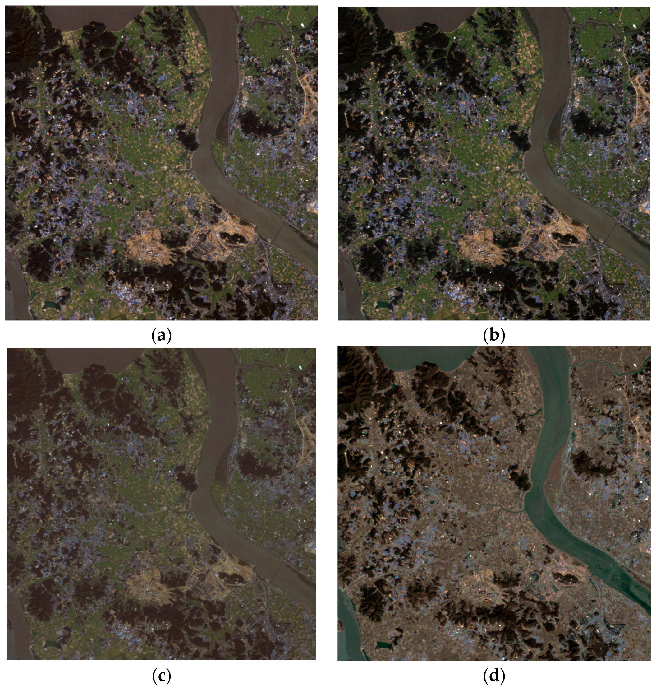
3.1. Study Sites and Data

The study sites were located in Gimpo (126.37°E, 37.29°N), which is located in the central-western part of South Korea. Gimpo has been a site of development since 2006. Therefore, for the intended detection of change before and after, two time-points were selected: 18 March 2005 for the reference image; and 27 September 2011 for the subject image. Figure 1a,b illustrates the RGB image of both the subject image and reference image. Moreover, the Korean Peninsula undergoes an increasing Leaf Area Index (LAI) trend beginning in March, and shows elevated LAI values in September. Thus, there are phenological variations between the two-time images [47]. The present research data are based on an image obtained from a Landsat-5 satellite Thematic Mapper (TM) sensor and the Global Digital Elevation Model (GDEM) V2 was obtained from the Advanced Spaceborne Thermal Emission and Reflection Radiometer (ASTER) sensor. In the case of the GDEM, the image obtained on 17 October 2011—which is temporally similar to the subject image—were utilized. At this time, one of the most important preprocessing steps for accurate normalization and change detection results is image registration [48], which matches the geometric location information of two images. The Landsat-5 TM images used in this study were the Level-1 precision and terrain corrected product (L1TP) that was corrected geometrically and topographically through co-registration [49]. Moreover, only areas without cloud or fog were extracted to avoid the influence of such weather conditions in the Landsat-5 TM image. Thus, from each image set, 600 × 600 pixels of the same location without cloud or fog were extracted to implement the experiment.

3.2. Methods

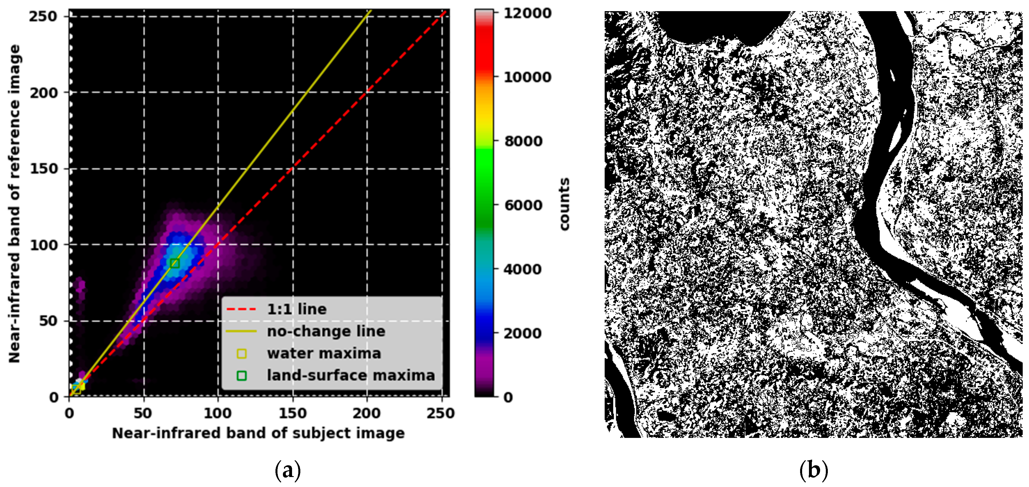
3.2.1. Automatic Detection of No-Change Pixel

To ensure that the no-change pixel selection process was independent from operator performance effects, this selection was carried out through an automatic process. In this study, we extracted the no-change set based on the scattergram used in NC regression. As mentioned above, the no-change pixels were identified in the scattergram between near-infrared bands for the subject and reference images. This method locates the statistical centers of water and land-surface clusters based on local maxima for the near-infrared bands in the scattergram [28]. The no-change set is defined as indicated in Equation (9) [50],

$$N{C}_{\mathrm{set}}=\left\{\left|{\mathit{y}}_{\mathbf{4}}-{\mathit{a}}_{{\mathbf{4}}_{\mathbf{0}}}{\mathit{x}}_{\mathbf{4}}-{\mathit{b}}_{{\mathbf{4}}_{\mathbf{0}}}\right|\le \mathrm{HVW}\right\},$$

(9)

where ${\mathit{a}}_{{\mathbf{4}}_{\mathbf{0}}}$ and ${\mathit{b}}_{{\mathbf{4}}_{\mathbf{0}}}$ are the initial normalization coefficients for the near-infrared band, obtained from the centers of the water and land-surface clusters; HVW is the corresponding half vertical width of the no-change regions in the scattergram, given the half perpendicular width (HPW) of the no-change region. The relationship between HVW and HPW is expressed by Equation (10) [25,28]:

$$\mathrm{HVW}=\mathrm{HPW}\sqrt{\mathbf{1}+{\mathit{a}}^{\mathbf{2}}{}_{{\mathbf{4}}_{\mathbf{0}}}}.$$

(10)

Next, it was assumed that the majority (>50%) of pixels in the images did not experience significant land-cover change between the two dates represented by the reference and subject images [25]. In addition, the obtained no-change set should have a correlation coefficient greater than 0.9 [12,13]. In this study, the center coordinate of the water cluster in the scattergram was (5, 5), and the center coordinate of the land surface in the scattergram was (71, 88). From these two coordinates, the initial normalization coefficients were acquired: ${\mathit{a}}_{{\mathbf{4}}_{\mathbf{0}}}=\mathbf{1.2575}$; and ${\mathit{b}}_{{\mathbf{4}}_{\mathbf{0}}}=-\mathbf{1.2878}$. The HPW value was selected as 11 to include 52.56% no-change regions (189,221 out of 360,000); the value of HVW was 17.6737, which was obtained with the ${\mathit{a}}_{{\mathbf{4}}_{\mathbf{0}}}$ value determined using Equation (10), and the correlation coefficient in the no-change set was 0.9740, which was greater than 0.9. Figure 2a shows the scattergram and no-change lines of the subject and reference images for the near-infrared bands. Each color in the scattergram indicates point density, with the corresponding colors representing numbers indicated in the legend. Thus, the areas that appear red have a higher point density than the areas that appear black. Figure 2b shows the no-change pixels selected based on the scattergram; the black area indicates non-change, and the white area represents change.

3.2.2. Radiometric Normalization Using Random Forest Regression

Many methods have been developed for relative radiometric normalization based on linear assumptions. However, as mentioned above, in cases where there are compositive differences in radiometric and phenological conditions, all of the corrections should be merged, and nonlinear transfer is necessary. For this reason, RF regression is used for nonlinear adjustment and radiometric correction using the no-change region. In this study, there were two main phases: training and prediction. The training stage refers to the process of constructing RF regression. For high-quality RF regression performance, the number of variables to be selected and tested for the best split when growing the trees (mtry) and the number of decision trees to be generated (ntree) should be optimized [22,23]. In this study, the mtry was set to the square root of the number of the input variable, as is commonly done [36].

Table 1. Description of the utilized explanatory variables.

Variable	Derived from
Band 1	Landsat 5 TM Band 1 pixel value
Band 2	Landsat 5 TM Band 2 pixel value
Band 3	Landsat 5 TM Band 3 pixel value
Band 4	Landsat 5 TM Band 4 pixel value
Band 5	Landsat 5 TM Band 5 pixel value
Band 7	Landsat 5 TM Band 7 pixel value
GLCM(Texture) of Bands 1–3	ASM, contrast, correlation, and entropy of 5 × 5 pixel neighborhood
Mean of Bands 1–3	Mean of 5 × 5 pixel neighborhood
Variance of Bands 1–3	Variance of 5 × 5 pixel neighborhood
Elevation	Derived from ASTER GDEM
Slope	Derived from ASTER GDEM using terrain function
Aspect	Derived from ASTER GDEM using terrain function

shows the selected explanatory variables. The total number of variables in this study was 27, and these variables were divided into two categories: variables extracted from the subject image; and variables extracted from the ASTER GDEM, which is temporally similar to the subject image. The variables selected for the former were Bands 1–5 and Band 7, which contained the spectral characteristics of the subject image. The gray-level co-occurrence matrix (GLCM) data were obtained using statistical values between a given pixel and the neighboring pixels, which showed the spatial characteristics of the pixels as a texture feature [51]. The statistical parameters applied in this study were angular second moment (ASM), contrast, correlation, and entropy, with better texture feature extraction in remote sensing [52]. ASM reflects the regularity and uniformity of image distribution; contrast reflects the depth and smoothness of the image texture structure; correlation reflects the similarity of the image texture in the horizontal or vertical direction, and entropy is a measure of image information that reflects the complexity of the texture distribution [52]; the mean pixel values, and the variance values, which are the main statistical values. Next, the GLCM, mean, and variance were obtained only for the R (Band 3), G (Band 2), and B (Band 1) values to be modeled for visual interpretation. For the latter group, elevation, slope, and aspect were selected. Digital elevation models (DEMs) are increasingly being used for visual and mathematical analysis of topography, landscape and landforms, as well as for modeling surface processes [53]. For these reasons, DEMs have become a core source of data for modeling in remote sensing, which provide information about the Earth’s surface and spatial distribution that cannot be obtained from images alone [54,55]. In particular, elevation, slope and aspect are the three primary topographic variables [56]. Slope and aspect data derived from DEMs are important variables used regularly in geographical information system for modeling purposes [54].

In the case of the ntree, a majority of studies have set the ntree value as 500 as the errors stabilize before this number of regression tree is achieved [23]. However, as investigated by Reference [57] the sensitivity of the number of trees showed that this parameter had no influence on the results. For this reason, 32, 64, 128, 256, 512, and 1024 were selected as the number of trees, and the optimal ntree value was derived by considering the performance of the RF regression calculated using Equation (8), as well as training time.

The prediction stage refers to the process of modeling radiometric and phenological normalized images. Modeling was performed using the RF regression obtained based on no-change region in the training stage. First, explanatory variables corresponding to each pixel position were acquired for all pixels of the subject image. Then, the obtained explanatory variable were used as the input values of the previously obtained RF regression. Finally, the normalized subject image was obtained through the obtained prediction values. At this time, only the R, G, and B bands were modeled for visual interpretation.

3.2.3. Accuracy Assessment of Radiometric Normalization

The quality of radiometric normalization can be statistically assessed based on the root mean squared error (RMSE) and R² value between pairs of corresponding bands. The RMSE is defined as shown in Equation (11),

$$\mathrm{RMSE}=\sqrt{\frac{{\displaystyle \sum }{({\mathit{y}}^{\mathit{N}}{}_{\mathit{i}}-{\mathit{y}}_{\mathit{i}})}^{\mathbf{2}}}{\mathit{n}}},$$

(11)

and the R² value is defined as in Equation (12),

$${\mathit{R}}^{\mathbf{2}}=\frac{{\displaystyle \sum }{({\mathit{y}}^{\mathit{N}}{}_{\mathit{i}}-\overline{{\mathit{y}}_{\mathit{i}}})}^{\mathbf{2}}}{{\displaystyle \sum }{({\mathit{y}}_{\mathit{i}}-\overline{{\mathit{y}}_{\mathit{i}}})}^{\mathbf{2}}},$$

(12)

where N is the total number of pixels in the scene. A lower RMSE value indicates a better fit and therefore better normalization results. The closer the R² value is to 1, the better the radiometric normalization process.

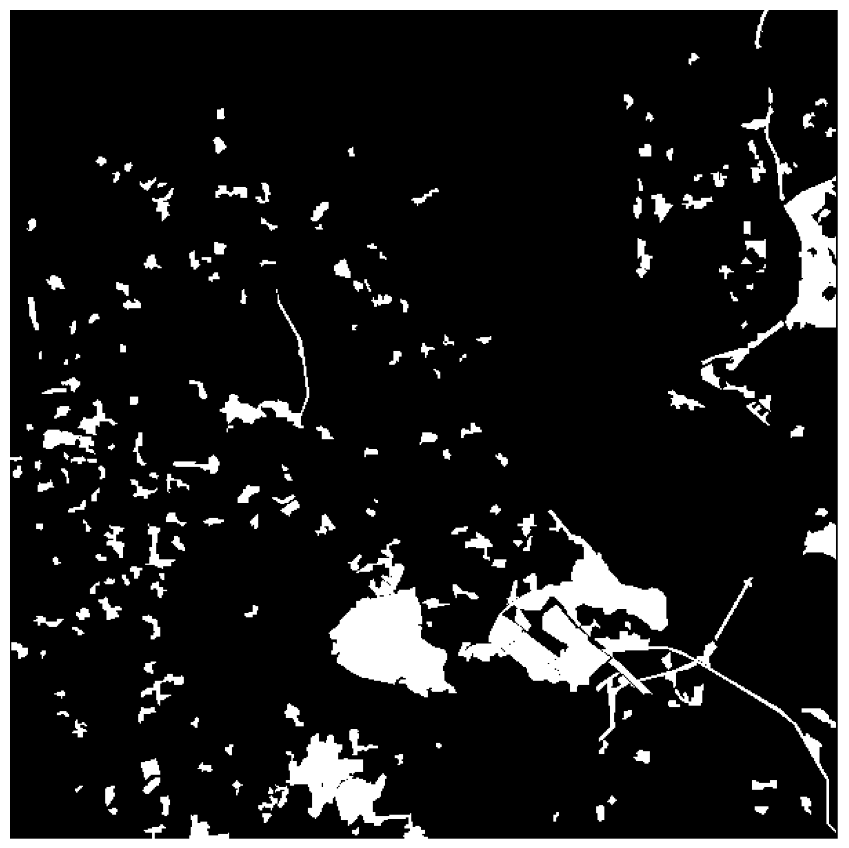
3.2.4. Change Detection

In this study, to investigate the use of the normalized subject images generated by RF regression in change detection, image differencing was performed with the reference images and compared with the change detection results of normalized subject images generated by linear regression. Image differencing is a method of subtracting pixel values from two images with a common coordinate system to observe changes between two different points in time. If the result of the operation has a positive or a negative value, change has occurred. If the value is close to 0, there has been no change. Then, the result of the operation is converted into a positive value by adding an arbitrary constant (offset value). The process of the image differencing is expressed as Equation (13) [3].

△x_d(i, j, k) = I₁(i, j, k) − I₂(i, j, k) + C

(13)

where I₁ is the pixel value at time 1; I₂ is the pixel value at time 2; C is the arbitrary constant; and i, j, and k are the row, column, and band, respectively. After the execution of image differencing, a threshold should be applied to distinguish between change and no change. In this study, Otsu’s method was used as it is the most practical method to determine the threshold value based on the brightness distribution of the input image [58]. At this time, given the characteristics of pixel-based change detection, there is a case of “salt-and-pepper”-type noise [59], which leads to the false detection of unchanged areas as change areas. To address this problem, segmentation was performed to determine the minimum object size, and noise was identified if the minimum object size was not satisfied in the change or no-change areas. For segmentation, a simple linear iterative clustering (SLIC) technique was used due to its relative simplicity and rapid computing speed [60]. SLIC is a segmentation method that entails the establishment of cluster space size, the creation of k cluster centers, measuring color and spatial distance, and designating the cluster center closest to each pixel [60,61]. Experiments were performed by setting the cluster space size to 5 × 5, 7 × 7, and 9 × 9 pixels.

To evaluate change detection accuracy, ground-truth data for the areas with actual change were distinguished from those with no change by carrying out manual digitizing. Manual digitizing generates ground-truth data by directly interpreting two date images through a combination of spatial properties (size, shape, texture, and pattern) and spectral properties (tone and color) [62]. The ground-truth data for this study are shown in Figure 3. Based on these ground-truth data, the user’s accuracy, producer’s accuracy, and overall accuracy were obtained. Overall accuracy is the percentage of samples correctly classified out of the entire sample. The user’s accuracy corresponds to the error of commission, whereas the producer’s accuracy corresponds to the error of omission. In other words, the user’s accuracy represents the proportion of correctly classified samples among the classified samples of the acquired map, and the producer’s accuracy represents the proportion of correctly classified samples among the ground-truth class samples [63].

4. Results

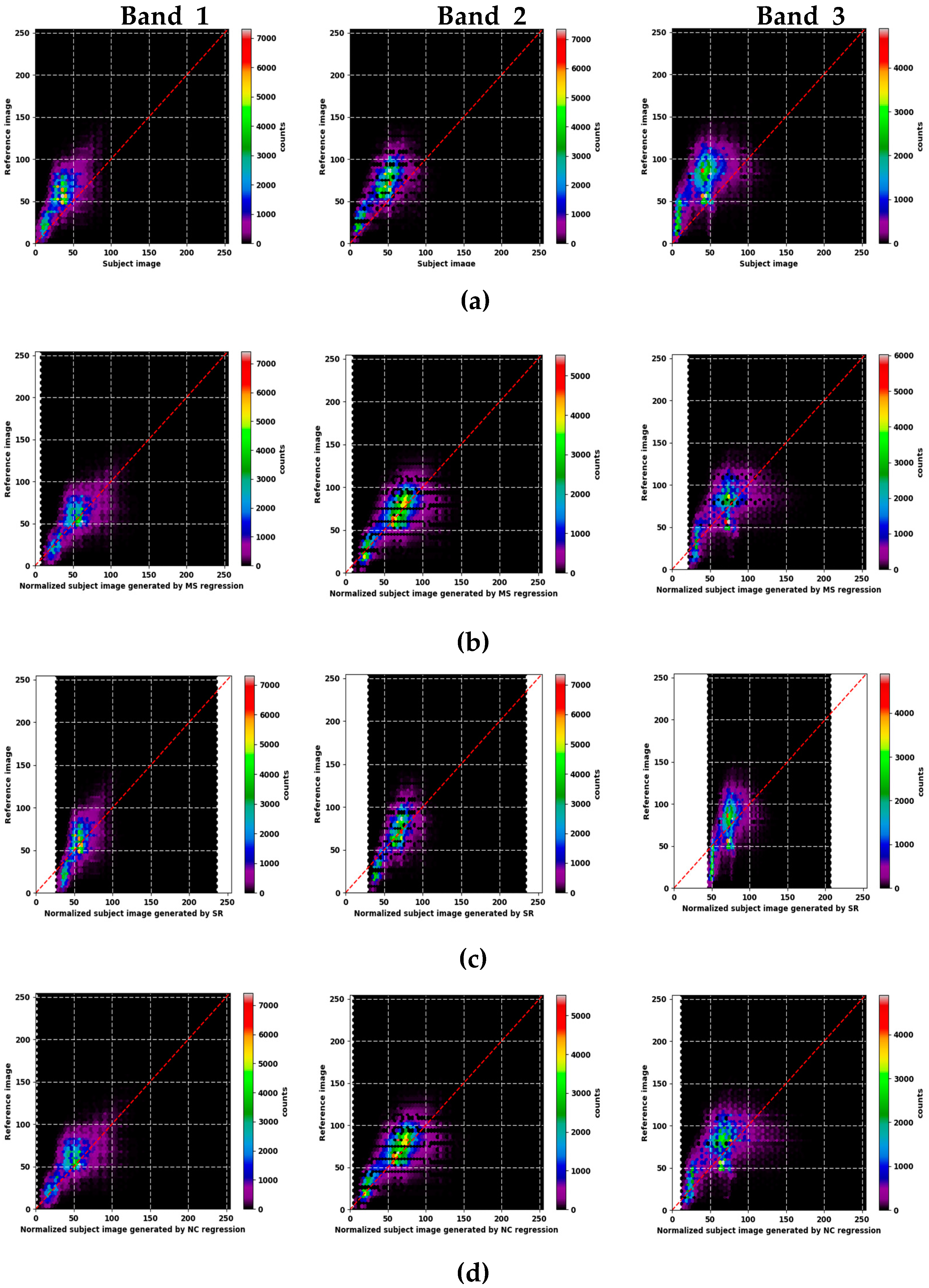
4.1. Assessment of Accuracy of the Linear Regression Method

For a comparison of the proposed method, R² and RMSE values were computed between normalized subject images generated by linear regression and reference images. The obtained R² and RMSE values are shown in

Table 2. Statistical results (R² and RMSE) of linear regression normalization.

Method	Band	R²	RMSE
Raw	Band 1	0.2994	29.2566
	Band 2	0.4219	29.5337
	Band 3	0.3894	39.2366
MS regression	Band 1	0.2998	22.9201
	Band 2	0.4231	22.3732
	Band 3	0.3915	27.6336
SR	Band 1	0.2994	20.7462
	Band 2	0.4219	20.3767
	Band 3	0.3895	24.3443
NC regression	Band 1	0.2998	23.0747
	Band 2	0.4232	22.4726
	Band 3	0.3915	28.0409

. The mean R² values of MS regression, SR, and NC regression were improved by 0.12%, 0.01%, and 0.13%, respectively, and the mean RMSE values were improved by 25.61%, 33.22%, and 24.93%, respectively, relative to the raw subject images. RMSE values were thus slightly improved, but R² values improved very little. The scattergrams of Band 1, Band 2 and Band 3 with the reference images were obtained to confirm the bias, as shown in Figure 4. Compared with the scattergram of the raw subject images, the bias was slightly reduced in the case of MS and NC regression, but bias was still present; almost no bias was removed in the case of SR.

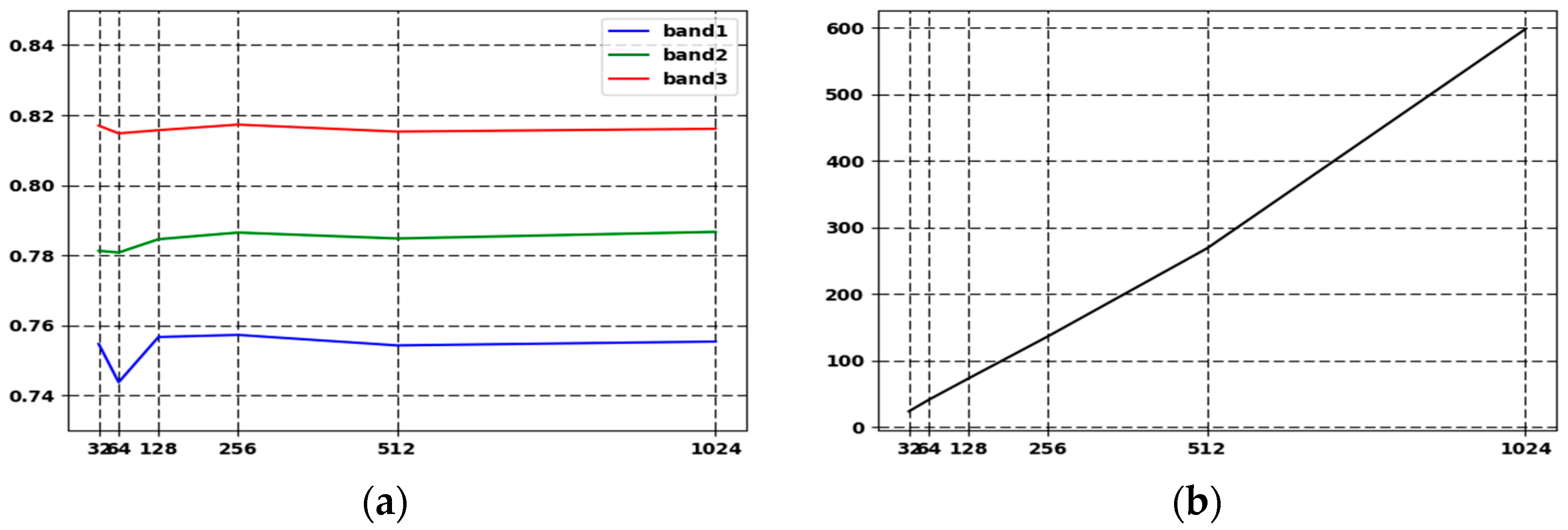
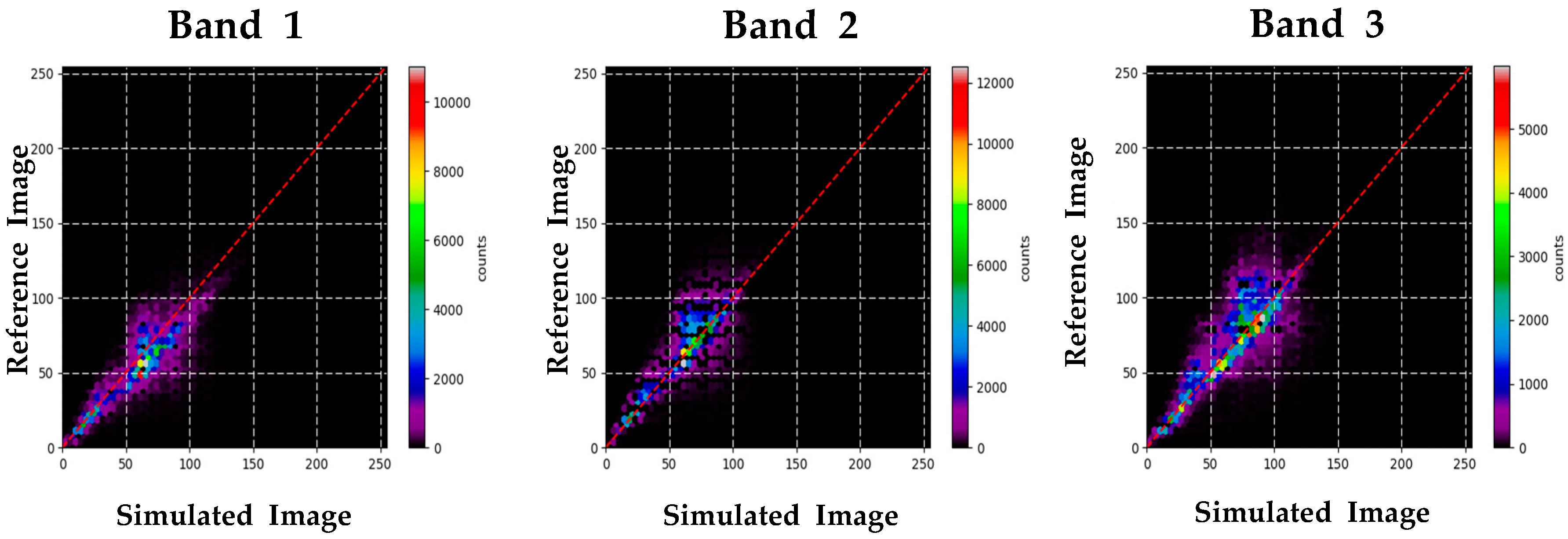
4.2. Assessment of Accuracy of Random Forest Regression

As mentioned in Section 3.2.2, to select the optimal ntree, six experiments were performed using 32, 64, 128, 256, 512, and 1024 trees. As shown in

Table 3. OOB-R² and training time of RF regression.

Tree Numbers	Band	OOB-R²	Training Time
32	Band 1	0.7547	23.6119 s
	Band 2	0.7813
	Band 3	0.8170
64	Band 1	0.7438	41.0407 s
	Band 2	0.7808
	Band 3	0.8148
128	Band 1	0.7567	73.1419 s
	Band 2	0.7846
	Band 3	0.8157
256	Band 1	0.7573	136.5000 s
	Band 2	0.7865
	Band 3	0.8173
512	Band 1	0.7543	268.7962 s
	Band 2	0.7848
	Band 3	0.8153
1024	Band 1	0.7554	598.1220 s
	Band 2	0.7867
	Band 3	0.8161

and Figure 5, the results indicate that the values of R² obtained through OOBs in Bands 1–3 were similar regardless of the number of trees. However, the training times increased in proportion to the number of trees. Based on the training time as well as the performance in terms of R², using 32 trees was verified to be most efficient; therefore, 32 was selected as the ntree. In addition, the variable importance was obtained for each band, and only the top five variables among the 27 included were extracted. For Band 1, the top five variables were Band 1, Band 2, Mean of Band 1, Band 3, and Mean Band 2, which corresponded to scores of 0.2023, 0.1440, 0.0825, 0.0797, and 0.0666, respectively. For Band 2, the top five variables were Mean of Band 2, Band 2, Band 1, Band 3, and Mean of Band 3, with corresponding scores being 0.1606, 0.1192, 0.1085, 0.1054, and 0.0836, respectively. In the case of Band 3, the top five variables were Band 5, Band 3, Band 1, Mean of Band 1, and Band 2, and the respective scores were 0.2131, 0.1376, 0.0999, 0.0736, and 0.0707. With the exception of Band 5 in Band 3, it was confirmed that the importance of Band 1, Band 2, Band 3, and Mean of Band variable was high. It should be noted, however, that the variable importance scores depend on the number of included variables. Removing or replacing predictors, for example, may change the importance scores as different inter-correlated variables could act as surrogates.

The scattergrams of Band 1, Band 2 and Band 3 between the normalized subject images generated by RF regression and the reference images are illustrated in Figure 6. The bias between these data was substantially reduced when compared to the scattergrams of normalized subject images generated by linear regression. In addition, to evaluate the performance of radiometric normalization, R² and RMSE values were computed between the normalized subject images generated by RF regression and the reference images. The obtained R² and RMSE values are shown in

Table 4. Statistical results (R² and RMSE) of RF regression normalization.

Method	Band	R²	RMSE
RF regression	Band 1	0.9040	8.2260
	Band 2	0.8982	8.5494
	Band 3	0.9249	7.9662

.

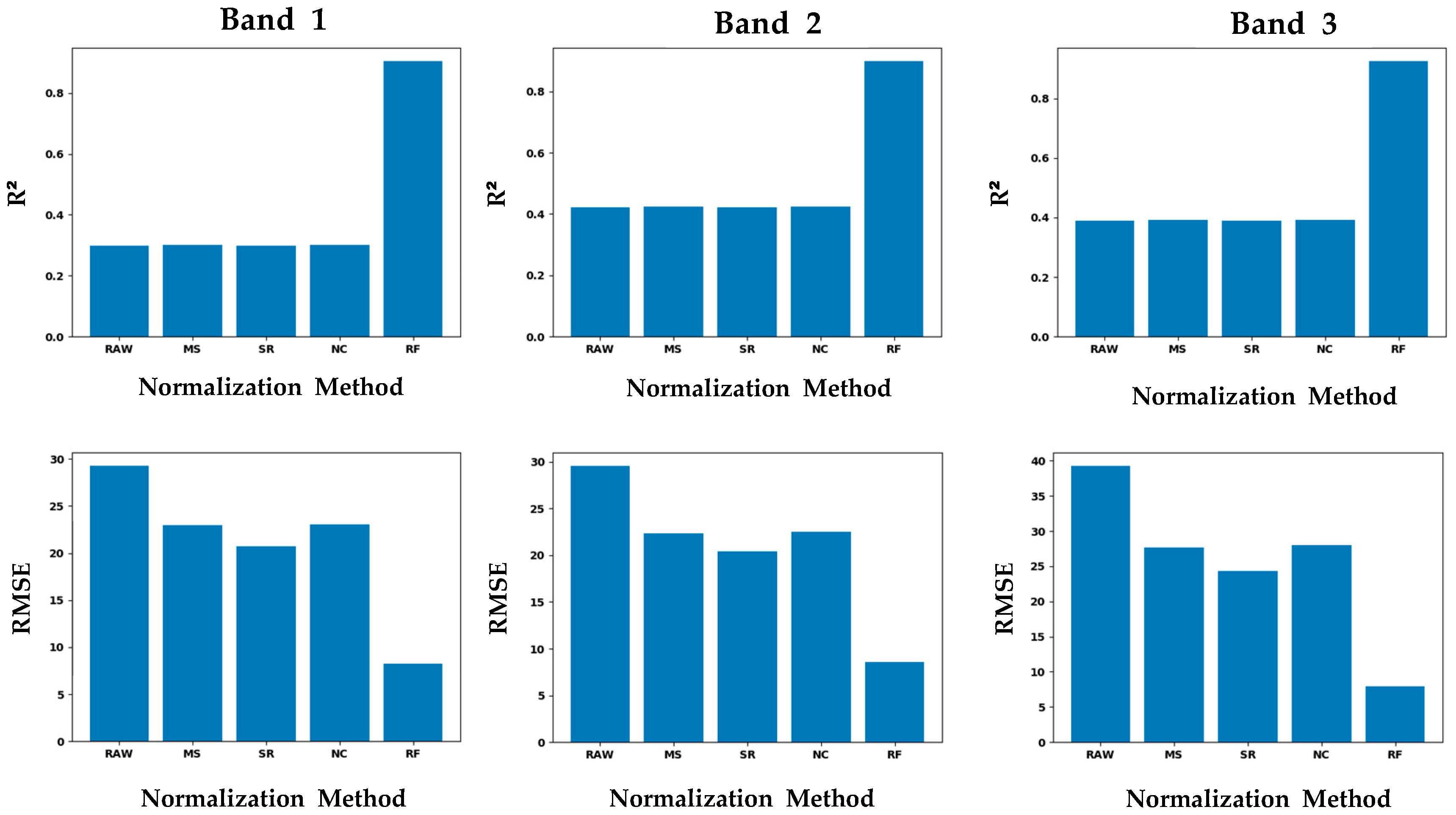
4.3. Comparison of Accuracy between Random Forest Regression and Linear Regression

To visually compare the results, normalized subject images were acquired, as illustrated in Figure 7. In the case of normalized subject images generated by linear regression, phenological normalization was not performed, whereas the normalized subject image generated by RF regression showed similar spectral characteristics to those of the reference image while retaining the spatial characteristics of the subject image. To compare the quantitative values, each R² and RMSE value was plotted as shown in Figure 8. The results showed that the performance of normalized subject images generated by RF regression was much better than that of the raw subject images and normalized subject images generated by linear regression. Applying RF regression improved the mean R² values in the raw, MS regression, SR, and NC regression by 53.88%, 53.75%, 53.87%, and 53.75%, respectively. In addition, the mean RMSE values were improved by 74.76%, 66.07%, 54.69%, and 66.37%, respectively.

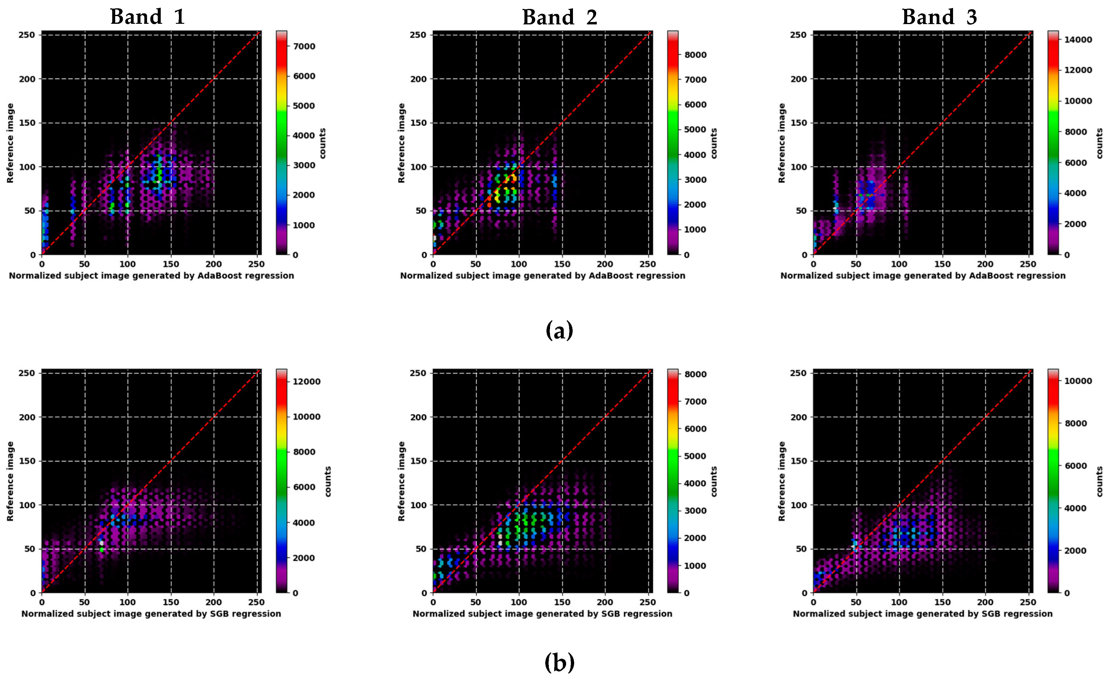
4.4. Assessment of Accuracy of Other Nonlinear Regression Method and Comparison of Accuracy with Random Forest Regression

As previously mentioned, two other nonlinear ensemble regression methods, AdaBoost regression and SGB regression, were compared for further evaluation of normalization using RF regression. For comparison under the same conditions, the same explanatory variables were used in RF regression, and the number of weak learner of AdaBoost regression and the number of trees of SGB regression were selected as 32, also used in the RF regression. The scattergram of the normalized image and reference image obtained through each regression are shown in Figure 9. It can be confirmed that the bias was still present and that the performances were significantly lower when compared with the scattergram of the normalized subject image generated by RF regression. The normalized subject image obtained by each regression is also shown in Figure 10. In the case of the normalized subject image generated by AdaBoost regression, it was confirmed that it did not contain any spectral characteristics of the reference image. In the case of the normalized subject image generated by SGB regression, it was similar to the spectral characteristics of the reference image, rather than the normalized subject image generated by AdaBoost regression, but the visual performance was significantly lower when compared with the normalized subject image generated by RF regression.

For the quantitative comparison, the normalization performance of the two images was obtained, as shown in

Table 5. Statistical results (R² and RMSE) of AdaBoost and SGB regression normalization.

Method	Band	R²	RMSE
AdaBoost regression	Band 1	0.3902	10.1300
	Band 2	0.4679	9.8297
	Band 3	0.3906	10.1142
SGB regression	Band 1	0.4657	9.8904
	Band 2	0.4705	10.5055
	Band 3	0.3856	10.0355

. The mean R² and RMSE of the normalized subject image generated by AdaBoost regression were 0.4162 and 10.0246, respectively. The mean R² and RMSE of the normalized subject image generated by SGB regression were 0.4406 and 10.1438, respectively. In comparison with the normalization performance of the RF regression, the normalization performance of AdaBoost regression was lower by 49.28% for R² and 18.06% for RMSE, and the normalization performance of SGB regression was lower by 46.84% for R² and 19.02% for RMSE. In other words, when compared with other nonlinear ensemble regressions, it confirmed that RF regression was stable and good normalization performance, and the additional usefulness of radiometric and phenological normalization using RF regression was judged.

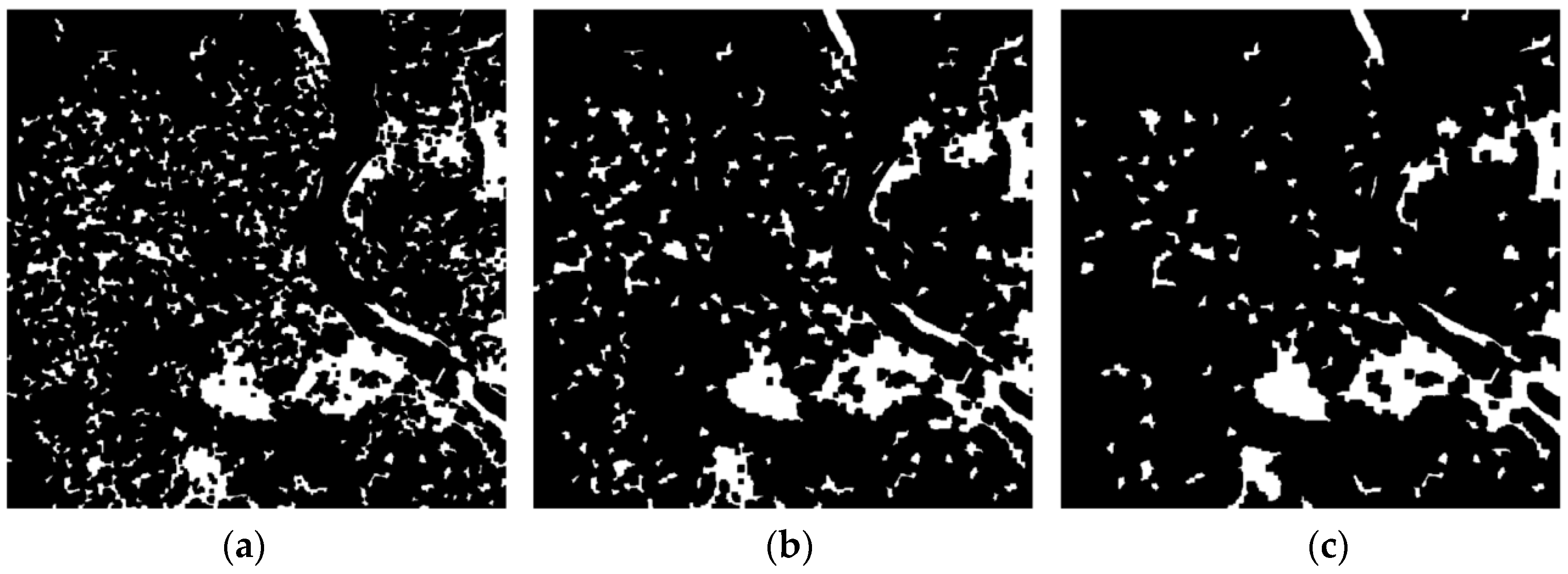
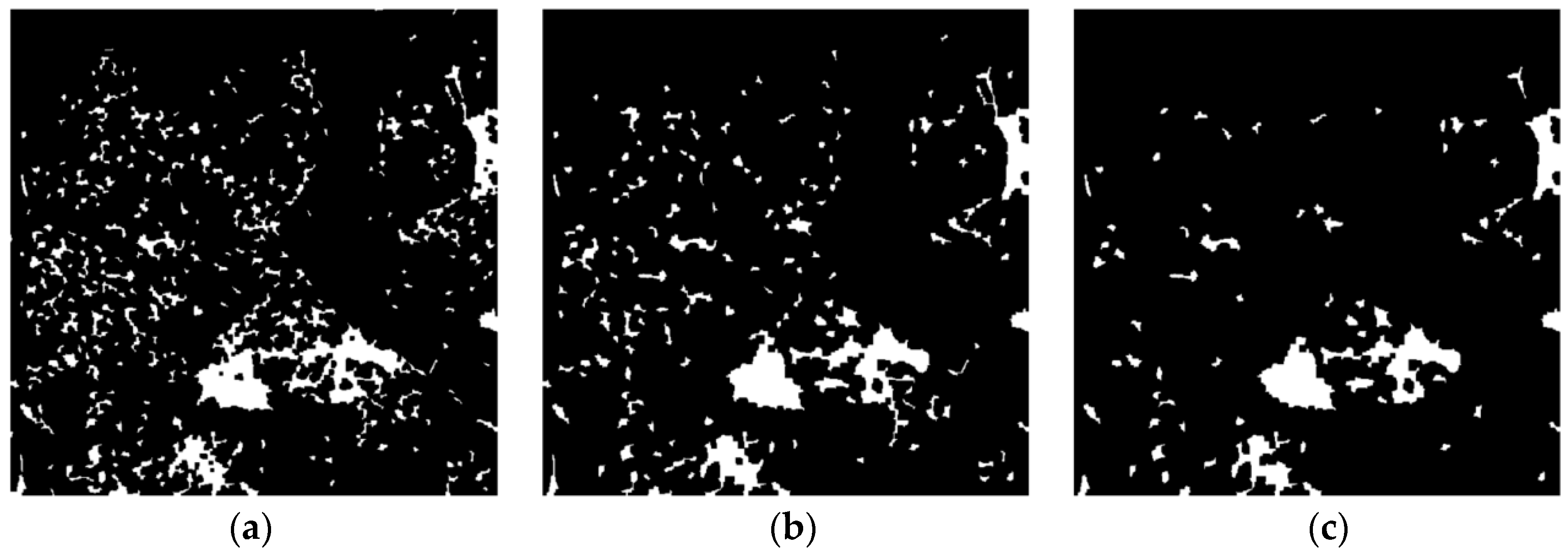
4.5. Analysis of Change Detection

To evaluate the effectiveness of the proposed method in change detection, image differencing was performed for each normalized subject image and reference image. Then, as mentioned above, SLIC was performed by setting cluster space sizes of 5 × 5, 7 × 7, and 9 × 9, and the noise of the change detection results were removed using the obtained minimum object sizes. The results are illustrated in Figure 11, Figure 12, Figure 13 and Figure 14. When interpreted visually with ground-truth data, the change detection results of the normalized subject images generated by linear regression are shown to be overestimated when compared with the change detection results of the normalized subject image generated by RF regression.

Quantitative comparisons of each change detection result are shown in

Table 6. Quantitative change detection result based on user’s accuracy, producer’s accuracy and overall accuracy.

Method		Overall Accuracy (%)	User’s Accuracy (%)		Producer’s Accuracy (%)
			Change	No-Change	Change	No-Change
MS	5 × 5	89.49	43.30	97.23	72.33	91.11
	7 × 7	90.99	48.23	96.81	67.34	93.21
	9 × 9	91.97	52.79	96.33	61.56	94.83
SR regression	5 × 5	70.33	19.19	96.93	76.48	69.75
	7 × 7	71.33	19.42	96.72	74.30	71.05
	9 × 9	73.86	20.36	96.37	70.19	74.21
NC regression	5 × 5	82.65	29.59	97.16	73.97	83.47
	7 × 7	84.63	31.74	96.70	68.66	86.13
	9 × 9	87.04	35.68	96.30	63.51	89.25
RF	5 × 5	94.00	63.59	97.20	70.44	96.21
	7 × 7	95.30	74.81	97.05	74.81	97.84
	9 × 9	95.07	81.22	95.94	55.45	98.80

. In the case of mean overall accuracy, the performance of change detection using normalized subject images generated by RF regression was 2.98%, 22.95%, and 10.02% higher than the change detection results obtained through MS regression, SR, and NC regression, respectively. In addition, the user’s accuracy was improved by 12.53%, 26.81%, and 20.45%, and the producer’s accuracy by 2.16%, 9.61%, and 4.78%, respectively. Thus, performance was significantly improved using the normalized subject images generated by RF regression for change detection.

5. Discussion

The objective of this paper was to evaluate the applicability of compositive normalization including radiometric and phenological using RF regression, which requires nonlinear modeling. This paper assessed the performance of RF regression based on statistical values and training time according to the number of trees. The number of trees used in experiments were 32, 64, 128, 256, 512, and 1024, and a total of six experiments were performed. The training time increased proportionally to the number of trees, whereas statistical value was not significantly affected by the number of trees. For this reason, when normalization using RF regression was performed, it was judged that the number of trees was not greatly influenced by the number of trees. Furthermore, in the case of variable importance, it was confirmed that the importance of GLCM, variance, and DEM-related variables were considerably small, and that the importance of Bands 1–3, and mean variables were generally large. In other words, the variables that had the greatest influence on the normalization were the pixels of the RGB bands, rather than data such as texture or topography. Next, normalization performance was assessed with a comparison to the R² and RMSE of conventional linear regression, MS regression, SR, NC regression, and compared with other nonlinear ensemble regressions (AdaBoost regression and SGB regression) for additional usefulness. Finally, the effectiveness of normalization using RF regression in change detection was confirmed by performing change detection.

The RF regression algorithms were credited for its nonlinear expression, stability, and satisfactory accuracy. First, the RF regression (which is characterized by nonlinear regression) provided accurate radiometric and phenological normalization. The visual analysis of the normalized subject images generated by conventional linear regression revealed that phenological normalization was not performed and the statistical values were also unsatisfactory. Unlike conventional linear regression approaches for normalization, the normalized subject image generated by the proposed method contained the spatial characteristics of the subject image and spectral characteristics of the reference image. Furthermore, it confirmed that the R² and RMSE values were significantly improved. Second, when compared with other nonlinear ensemble regression, RF regression was able to minimize overfitting and handle high dimensional data. Both the AdaBoost and SGB regressions were significantly lower than those of RF regression when compared on visual and statistical values. That is, when compared with other ensemble regressions, it was confirmed that normalization through RF regression was stable. Third, the normalized subject image generated by RF regression in change detection provided satisfactory accuracy. When the change detection was performed on each normalized subject image, the overall accuracy and user accuracy were significantly improved and the producer accuracy was slightly improved by using the normalized subject image generated by RF regression when compared with the normalized subject image generated by conventional linear regression. At this time, the producer’s accuracy was slightly improved when compared with the overall accuracy and user accuracy, which was due to the overestimation of change regions in the normalization image of the linear regression approaches. In other words, if phenological normalization was not performed properly, there was a potential risk of producing meaningless information in change detection. Therefore, the proposed method performed the normalization of nonlinear relations properly, especially when compared to nonlinear ensemble regression as well as conventional linear regression, and was also useful for change detection.

6. Conclusions

In this paper, we have addressed the issue of normalizing radiometric and phenological conditions. To achieve this goal, RF regression was selected from among the many potential techniques that can model nonlinear relationships. The comparison results based on visual and statistical values showed that normalization through RF regression produced a significantly satisfactory performance. Compared with the normalization performance of conventional linear regression, R² and RMSE were improved on average by 53.81% and 65.47%, respectively. In comparison to the normalization performance of the other nonlinear ensemble regressions, R² and RMSE on average were higher by 48.01% and 18.54%, respectively. In addition, when compared with the change detection results of a normalized subject image generated by conventional linear regression, 11.98% of the overall accuracy, 19.93% of the user’s accuracy, and 5.52% of the producer’s accuracy were improved on average. Based on the findings of this study, we concluded that normalization through RF regression had been performed appropriately.

In future studies, efforts should be made to ensure the development of technology to improve the RF regression performance. In particular, the effects of the variable importance and combinations of explanatory variables used for RF regression should be further analyzed. Moreover, the usefulness of the proposed approach should be validated by obtaining sufficient reference images for each season and time period, and by utilizing images acquired by other satellites and sensors. In addition, it is necessary to verify the applicability of this method with complex structures by applying RF regression to high-resolution images.

References

1. Alberga, V. Similarity Measures of Remotely Sensed Multi-Sensor Images for Change Detection Applications. Remote Sens. 2009, 1, 122–143. [Google Scholar] [CrossRef]
2. Almutairi, A.; Warner, T.A. Change Detection Accuracy and Image Properties: A Study Using Simulated Data. Remote Sens. 2010, 2, 1508–1529. [Google Scholar] [CrossRef]
3. Singh, A. Digital Change Detection Technique Using Remotely-Sensed Data. Int. J. Remote Sens. 1989, 10, 989–1003. [Google Scholar] [CrossRef]
4. Zhou, L.; Cao, G.; Li, Y.; Shang, Y. Change Detection Based on Conditional Random Field with Region Connection Constraints in High-Resolution Remote Sensing Images. IEEE J. Sel. Top. Appl. Earth Obs. Remote Sens. 2016, 9, 3478–3488. [Google Scholar] [CrossRef]
5. Ajadi, O.A.; Meyer, F.J.; Webley, P.W. Change Detection in Synthetic Aperture Radar Images Using a Multiscale-Driven Approach. Remote Sens. 2016, 8, 482. [Google Scholar] [CrossRef]
6. Rokni, K.; Ahmad, A.; Solaimani, K.; Hazini, S. A New Approach for Surface Water Change Detection: Integration of Pixel Level Image Fusion and Image Classification Techniques. Int. J. Appl. Earth Obs. Geoinf. 2014, 34, 226–234. [Google Scholar] [CrossRef]
7. Song, C.; Woodcock, C.E.; Seto, K.C.; Lenney, M.P.; Macomber, S.A. Classification and Change Detection Using Landsat TM Data: When and How to Correct Atmospheric Effects? Remote Sens. Environ. 2001, 75, 230–244. [Google Scholar] [CrossRef]
8. Pudale, S.R.; Bhole, U.V. Comparative Study of Relative Normalization Technique for Resourcesat1 LISS III Sensor Images. In Proceedings of the International Conference on Computational Intelligence and Multimedia Applications 2007, Sivakasi, India, 13–15 December 2007; pp. 233–239. [Google Scholar]
9. Bao, N.; Lechner, A.M.; Fletcher, A.; Mellor, A.; Mulligan, D.; Bai, Z. Comparison of Relative Radiometric Normalization Methods Using Pseudo-Invariant Features for Change Detection Studies in Rural and Urban Landscapes. J. Appl. Remote Sens. 2012, 6, 063578. [Google Scholar] [CrossRef]
10. Carvalho, O.A.; Guimaraes, R.F.; Silva, N.C.; Gillespie, A.R.; Gomes, A.T.; Silva, C.R.; Carvalho, P.F. Radiometric Normalization of Temporal Images Combining Automatic Detection of Pseudo-Invariant Features from the Distance and Similarity Spectral Measures, Density Scatterplot Analysis, and Robust Regression. Remote Sens. 2013, 5, 2763–2794. [Google Scholar] [CrossRef]
11. Liu, Y.; Yano, T.; Nishiyama, S.; Kimura, R. Radiometric Correction for Linear Change-Detection Technique: Analysis in Bi-temporal Space. Int. J. Remote Sens. 2007, 28, 5143–5157. [Google Scholar] [CrossRef]
12. Biday, S.G.; Bhosle, U. Radiometric Correction of Multitemporal Satellite Imagery. J. Comput. Sci. 2010, 6, 201–213. [Google Scholar] [CrossRef]
13. Du, Y.; Teillet, P.M.; Cihlar, J. Radiometric Normalization of Multitemporal High-Resolution Satellite Image with Quality Control for Land Cover Change Detection. Remote Sens. Environ. 2002, 82, 123–134. [Google Scholar] [CrossRef]
14. Schott, J.R.; Salvaggion, C.; Volchok, W.J. Radiometric Scene Normalization Using Pseudo Invariant Features. Remote Sens. Environ. 1988, 26, 1–14. [Google Scholar] [CrossRef]
15. Rahman, M.M.; Hay, G.J.; Couloginer, I.; Hemachandran, B.; Bailin, J. An Assessment of Polynomial Regression Techniques for the Relative Radiometric Normalization (RRN) of High-Resolution Multi-Temporal Airborne Thermal Infrared (TIR) Imagery. Remote Sens. 2014, 6, 11810–11828. [Google Scholar] [CrossRef]
16. Zheng, Y.; Zhang, J.; VanGenderen, K.L. Change Detection Approach to SAR and Optical Image Integration. Int. Arch. Photogramm. Remote Sens. 2008, XXXVII Pt B7, 1077–1084. [Google Scholar]
17. Brieman, L. Random Forests. Mach. Learn. 2001, 45, 5–32. [Google Scholar] [CrossRef]
18. Rodriguez-Galiano, V.F.; Chica-Rivas, M. Evaluation of Different Machine Learning Methods for Land Cover Mapping of a Mediterranean Area Using Multi-Seasonal Landsat Images and Digital Terrain Models. Int. J. Digit. Earth 2014, 7, 492–509. [Google Scholar] [CrossRef]
19. Wang, L.; Zhou, X.; Zhu, X.; Dong, Z.; Guo, W. Estimation of Biomass in Wheat Using Random Forest Regression Algorithm and Remote Sensing Data. Crop J. 2016, 4, 212–219. [Google Scholar] [CrossRef]
20. Ahmadlou, M.; Delavar, M.R.; Shafizadeh-Moghadam, H.; Tayyebi, A. Modeling Urban Dynamics Using Random Forest: Implementing Roc and Toc for Model Evaluation. Int. Arch. Photogramm. Remote Sens. Spat. Inf. Sci. 2016, XLI-B2, 285–290. [Google Scholar] [CrossRef]
21. Guan, H.; Yu, J.; Li, J.; Luo, L. Random Forest-Based Feature Selection for Land-Use Classification Using Lidar Data and Orthoimagery. Int. Arch. Photogramm. Remote Sens. Spat. Inf. Sci. 2012, XXXIX-B7, 203–208. [Google Scholar] [CrossRef]
22. Hultquist, C.; Chen, G.; Zhao, K. A Comparison of Gaussian Process Regression, Random Forests and Support Vector Regression for Burn Severity Assessment in Diseased Forests. Remote Sens. Lett. 2014, 5, 723–732. [Google Scholar] [CrossRef]
23. Belgiu, M.; Dragut, L. Random Forest in Remote Sensing: A Review of Applications and Future Directions. ISPRS J. Photogramm Remote Sens. 2015, 114, 24–31. [Google Scholar] [CrossRef]
24. Culter, D.R.; Edwards, T.C.; Beard, K.H.; Culter, A.; Hess, K.T.; Gibson, J.C. Random Forests for Classification in Ecological Society of America. Ecology 2007, 88, 2783–2792. [Google Scholar] [CrossRef]
25. Yuan, D.; Elvidge, C.D. Comparison of Relative Radiometric Normalization Techniques. ISPRS. J. Photogramm. Remote Sens. 1996, 51, 117–126. [Google Scholar] [CrossRef]
26. Olthof, I.; Pouliot, D.; Fernandes, R.; Latifovic, R. Landsat-7 ETM+ Radiometric Normalization Comparison for Northern Mapping Applications. Remote Sens. Environ. 2005, 95, 388–398. [Google Scholar] [CrossRef]
27. Sadeghi, V.; Ebadi, H.; Farshid, F.A. A New Model for Automatic Normalization of Multi-temporal Satellite Images Using Artificial Neural Network and Mathematical Methods. Appl. Math. Model. 2013, 37, 6437–6445. [Google Scholar] [CrossRef]
28. Elvidge, C.D.; Yuan, D.; Weerackoon, R.D.; Lunetta, R.S. Relative Radiometric Normalization of Landsat Multispectral Scanner(MSS) Data Using an Automatic Scattergram Controlled Regression. Photogramm. Eng. Remote Sens. 1995, 61, 1255–1260. [Google Scholar]
29. Ya’allah, S.M.; Saradjian, M.R. Automatic Normalization of Satellite Images Using Unchanged Pixels within Urban Areas. Inf. Fusion. 2005, 6, 235–241. [Google Scholar] [CrossRef]
30. Prasad, A.M.; Iverson, L.R.; Liaw, A. Newer Classification and Regression Tree Techniques: Bagging and Random Forests for Ecological Prediction. Ecosystems 2006, 9, 181–199. [Google Scholar] [CrossRef]
31. Shataee, S.; Kalbi, S.; Fallah, A.; Pelz, D. Forest Attribute Imputation Using Machine Learning Methods and ASTER Data: Comparison of K-NN, SVR, Random Forest Regression Algorithms. Int. J. Remote Sens. 2012, 33, 6254–6280. [Google Scholar] [CrossRef]
32. Peters, J.; Baets, B.D.; Verhoest, N.E.C.; Samson, R.; Degroeve, S.; Becker, P.D.; Huybrechts, W. Random Forests as a Tool for Ecohydrological Distribution Modeling. Ecol. Model. 2007, 207, 304–318. [Google Scholar] [CrossRef]
33. Abdel-Rahman, E.M.; Ahmed, F.B.; Ismail, R. Random Forest Regression and Spectral Band Selection for Estimating Surgarcane Leaf Nitrogen Concentration using EO-1 Hyperion Hyperspectral Data. Int. J. Remote Sens. 2013, 34, 712–728. [Google Scholar] [CrossRef]
34. Hutengs, C.; Vohland, M. Downscaling Land Surface Temperatures at Regional Scales with Random Forest Regression. Remote Sens. Environ. 2016, 178, 127–141. [Google Scholar] [CrossRef]
35. Gromping, U. Variable Importance Assessment in Regression: Linear Regression versus Random Forest. Am. Stat. 2009, 63, 308–319. [Google Scholar] [CrossRef]
36. Rodriguez-Galiano, V.; Sanchez-Castillo, M.; Chica-olmo, M.; Chica-Rivas, M. Machine Learning Predictive Models for Mineral Prospectivity: An Evaluation of Neural Networks, Random Forest, Regression Trees and Support Vector Machine. Ore Geol. Rev. 2015, 71, 804–818. [Google Scholar] [CrossRef]
37. Gislason, P.O.; Benediktsson, J.A.; Sveinsson, J.R. Random Forests for Land Cover Classification. Pattern Recogn. Lett. 2006, 27, 294–300. [Google Scholar] [CrossRef]
38. Pal, M. Random Forest Classifier for Remote Sensing Classification. Int. J. Remote Sens. 2005, 26, 217–222. [Google Scholar] [CrossRef]
39. Freund, Y.; Schapire, R.E. Experiments with a New Boosting Algorithm. In Proceedings of the Thirteenth International Conference on International Conference on Machine Learning, Bari, Italy, 3–6 July 1996; pp. 148–156. [Google Scholar]
40. Pardoe, D.; Stone, P. Boosting for Regression Transfer. In Proceedings of the 27th International Conference on Machine Learning, Haifa, Israel, 21–25 June 2010; pp. 863–870. [Google Scholar]
41. Avnimelech, R.; Intrator, N. Boosting Regression Estimators. Neural Comput. 1999, 11, 499–520. [Google Scholar] [CrossRef] [PubMed]
42. Drucker, H. Improving Regressors Using Boosting Techniques. In Proceedings of the Fourteenth International Conference on Machine Learning, San Francisco, CA, USA, 8–12 July 1997; pp. 107–115. [Google Scholar]
43. Friedman, J.H. Greedy Function Approximation: A Gradient Boosting Machine. Ann. Stat. 2001, 29, 1189–1232. [Google Scholar] [CrossRef]
44. Friedman, J.H. Stochastic Gradient Boosting. Comput. Stat. Data Anal. 2002, 38, 367–378. [Google Scholar] [CrossRef]
45. Moisen, G.; Freeman, E.A.; Blackard, J.A.; Frescino, T.S.; Zimmermann, N.E.; Edwords, T.C., Jr. Prediction Tree Species Presence and Basal Area in Utah: A Comparison of Stochastic Gradient Boosting, Generalized Addictive Models, and Tree-Based Method. Ecol. Model. 2006, 199, 176–187. [Google Scholar] [CrossRef]
46. Lawrence, R.; Bunn, A.; Powell, S.; Zambon, M. Classification of Remotely Sensed Imagery Using Stochastic Gradient Boosting as a Refinement of Classification Tree Analysis. Remote Sens. Environ. 2004, 90, 331–336. [Google Scholar] [CrossRef]
47. Kim, S.H.; Park, J.H.; Woo, C.S.; Lee, K.S. Analysis of Temporal Variability of MODIS Leaf Area Index (LAI) Product over Temperate Forest in Korea. In Proceedings of the IEEE International Geoscience and Remote Sensing Symposium, Seoul, Korea, 29 July 2005; pp. 4343–4346. [Google Scholar]
48. Wang, Q.; Zou, C.; Yuan, Y.; Lu, H.; Yan, P. Image Registration by Normalized Mapping. Neurocomputing 2013, 101, 181–189. [Google Scholar] [CrossRef]
49. Chen, G.; He, Y.; Santis, A.D.; Li, G.; Cobb, R.; Meentemeyer, R.K. Assessing the Impact of Emerging Forest Disease on Wildfire Using Landsat and KOMPSAT-2 Data. Remote Sens. Environ. 2017, 195, 218–229. [Google Scholar] [CrossRef]
50. Hong, G.; Zhang, Y. A Comparative Study on Radiometric Normalization Using High Resolution Satallite Images. Int. J. Remote Sens. 2008, 29, 425–438. [Google Scholar] [CrossRef]
51. Mohanaiah, P.; Sathyanarayana, P.; GuruKumar, L. Image Texture Feature Extraction Using GLCM Approach. Int. J. Sci. Res. 2013, 3, 1–5. [Google Scholar]
52. Zhang, X.; Cui, J.; Wang, W.; Lin, C. A Study for Texture Feature Extraction of High-Resolution Satellite Images Based on a Direction Measure and Gray Level Co-Occurrence Matrix Fusion Algorithm. Sensors 2017, 17, 1474. [Google Scholar] [CrossRef] [PubMed]
53. Kamp, U.; Bolch, T.; Olsenholler, J. Geomorphometry of Cerro Sillajhuay (Andes, Chile/Bolivia): Comparison of Digital Elevation Models (DEMs) from ASTER Remote Sensing Data and Contour Maps. Geocarto Int. 2005, 20, 23–33. [Google Scholar] [CrossRef]
54. Kumar, L. Effect of Rounding off Elevation Values on the Calculation of Aspect and Slope from Gridded Digital Elevation Model. J. Spat. Sci. 2013, 58, 91–100. [Google Scholar] [CrossRef]
55. Zhang, Z.; Collie, F.C.; Ou, X.; Wulf, R.D. Integration of Satellite Imagery, Topography and Human Disturbance Factors Based on Canonical Correspondence Analysis Ordination for Mountain Vegetation Mapping: A Case Study in Yunnan, China. Remote Sens. 2014, 6, 1026–1056. [Google Scholar] [CrossRef] [Green Version]
56. Mokarram, M.; Sathyamoorthy, D. Modeling the Relationship between Elevation, Aspect and Spatial Distribution of Vegetation in the Darab Mountain, Iran Using Remote Sensing Data. Model. Earth Syst. Environ. 2015, 1, 30. [Google Scholar] [CrossRef]
57. Du, P.; Samat, A.; Waske, B.; Liu, S.; Li, Z. Random Forest and Rotation Forest for Fully Polarized SAR Image Classification Using Polarimetric and Spatial Feature. ISPRS J. Photogramm. Remote Sens. 2015, 105, 38–53. [Google Scholar] [CrossRef]
58. Otsu, M.A. Threshold Selection Method from Gray-Level Histograms. IEEE Trans. Syst. Man Cybern. 1979, 9, 62–66. [Google Scholar] [CrossRef]
59. Blachke, T. Object Based Image Analysis for Remote Sensing. ISPRS. J. Photogramm. Remote Sens. 2010, 65, 2–16. [Google Scholar] [CrossRef]
60. Achanta, R.; Shaji, A.; Smith, K.; Lucchi, A.; Fua, P.; Susstrunk, S. SLIC Superpixels Compared to State-of-the-Art Superpixel Methods. IEEE Trans. Pattern Anal. Mach. Intell. 2012, 34, 2274–2282. [Google Scholar] [CrossRef] [PubMed]
61. Toro, C.A.O.; Martin, C.G.; Pedrero, A.G. Superpixel-Based Roughness Measure for Multispectral Satellite Image Segmentation. Remote Sens. 2015, 7, 14620–14645. [Google Scholar] [CrossRef]
62. Mathieu, R.; Aryal, J.; Change, A.K. Object-Based Classification of IKONOS Imagery for Mapping Large-Scale Vegetation Communities in Urban Areas. Sensors 2007, 7, 2860–2880. [Google Scholar] [CrossRef] [PubMed]
63. Story, M. Accuracy Assessment: A User’s Perspective. Photogramm. Eng. Remote Sens. 1986, 52, 397–399. [Google Scholar]
Figure 1. Study area: (a) subject image (27 September 2011); and (b) reference image (18 March 2005).
Remotesensing 09 01163 g001
Figure 2. (a) Scattergram of near-infrared bands for subject image and reference image; and (b) the location of selected no-change regions.
Remotesensing 09 01163 g002
Figure 3. Ground truth data obtained by manual digitizing.
Remotesensing 09 01163 g003
Figure 4. Scattergram of Band 1, Band 2 and Band 3 with reference image: (a) raw subject image; (b) normalized subject image generated by MS regression; (c) normalized subject image generated by SR; and (d) normalized subject image by NC regression.
Remotesensing 09 01163 g004
Figure 5. RF regression implementation graph: (a) OOB-R2; and (b) training time.
Remotesensing 09 01163 g005
Figure 6. Scattergram of Band 1, Band 2 and Band 3 between normalized subject image generated by RF regression and reference image.
Remotesensing 09 01163 g006
Figure 7. Normalized subject image: (a) MS regression; (b) SR; (c) NC regression; and (d) RF regression.
Remotesensing 09 01163 g007
Figure 8. Comparison of R2 and RMSE for the raw image and normalized subject image generated by different linear regressions and RF regression.
Remotesensing 09 01163 g008
Figure 9. Scattergram of Band 1, Band 2, and Band 3 with reference image: (a) AdaBoost regression; and (b) SGB regression.
Remotesensing 09 01163 g009
Figure 10. Normalized subject image: (a) AdaBoost regression; and (b) SGB regression.
Remotesensing 09 01163 g010
Figure 11. Image differencing results between normalized subject image generated by MS and reference image: (a) noise reduction using SLIC 5 × 5; (b) noise reduction using SLIC 7 × 7; and (c) noise reduction using SLIC 9 × 9.
Remotesensing 09 01163 g011
Figure 12. Image differencing results between normalized subject image generated by SR and reference image: (a) noise reduction using SLIC 5 × 5; (b) noise reduction using SLIC 7 × 7; and (c) noise reduction using SLIC 9 × 9.
Remotesensing 09 01163 g012
Figure 13. Image differencing results between normalized subject image generated by NC and reference image: (a) noise reduction using SLIC 5 × 5; (b) noise reduction using SLIC 7 × 7; and (c) noise reduction using SLIC 9 × 9.
Remotesensing 09 01163 g013
Figure 14. Image differencing results between normalized subject image generated by RF regression and reference image: (a) noise reduction using SLIC 5 × 5; (b) noise reduction using SLIC 7 × 7; and (c) noise reduction using SLIC 9 × 9.
Remotesensing 09 01163 g014