Hyperspectral Image Spatial Super-Resolution via 3D Full Convolutional Neural Network

Abstract

Hyperspectral images are well-known for their fine spectral resolution to discriminate different materials. However, their spatial resolution is relatively low due to the trade-off in imaging sensor technologies, resulting in limitations in their applications. Inspired by recent achievements in convolutional neural network (CNN) based super-resolution (SR) for natural images, a novel three-dimensional full CNN (3D-FCNN) is constructed for spatial SR of hyperspectral images in this paper. Specifically, 3D convolution is used to exploit both the spatial context of neighboring pixels and spectral correlation of neighboring bands, such that spectral distortion when directly applying traditional CNN based SR algorithms to hyperspectral images in band-wise manners is alleviated. Furthermore, a sensor-specific mode is designed for the proposed 3D-FCNN such that none of the samples from the target scene are required for training. Fine-tuning by a small number of training samples from the target scene can further improve the performance of such a sensor-specific method. Extensive experimental results on four benchmark datasets from two well-known hyperspectral sensors, namely hyperspectral digital imagery collection experiment (HYDICE) and reflective optics system imaging spectrometer (ROSIS) sensors, demonstrate that our proposed 3D-FCNN outperforms several existing SR methods by ensuring higher quality both in reconstruction and spectral fidelity.

1. Introduction

Hyperspectral remote sensing usually collects reflectance information of objects in hundreds of contiguous bands over a certain electromagnetic spectrum. It collects images with a very high spectral resolution, enabling a fine discrimination of different objects by their spectral signatures. However, due to the limitation of imaging sensor technologies, signal to noise ratio (SNR) and time constraints, there exists a trade-off between the spatial resolution and spectral resolution. Consequently, hyperspectral images (HSIs) are often acquired under a relatively low spatial resolution, degrading their performance in practical applications, including mineralogy, manufacturing and surveillance. Therefore, it is highly desirable to increase the spatial resolution of HSIs via post-processing.

In general, there are several ways to improve spatial resolution of HSIs: (1) image fusion with other high-spatial-resolution sources; (2) sub-pixel based analysis; and (3) single-image super-resolution (SR). The first two approaches have been widely exploited in hyperspectral applications. When an auxiliary image with a higher spatial resolution is available, such as a panchromatic image or multispectral image, image fusion can be applied for spatial-resolution enhancement. Statistics based fusion techniques are firstly proposed, such as maximum a posteriori (MAP) estimation, stochastic mixing model based method, etc. [1,2,3]. Recently, dictionary-based fusion methods dominate hyperspectral and multispectral image fusion, including spectral dictionary [4,5,6] and spatial dictionary based methods, but they cannot effectively utilize both spatial and spectral information equally. The Spatial–Temporal remotely sensed Images and land cover Maps Fusion Model (STIMFM) was proposed to produce land cover maps at both fine spatial and temporal resolutions using a series of coarse spatial resolution images together with a few fine spatial resolution land cover maps that pre- and post-date the series of coarse spatial resolution images [7]. The major limitation in these fusion techniques for HSI spatial-resolution enhancement is that an auxiliary co-registered image with a higher spatial resolution is required, which may be unavailable in practice.

Sub-pixel based analysis aims to exploit the information in the area covered by a pixel for different applications. Spectral mixture analysis (SMA) intends to estimate fractional abundance of pure ground objects within a mixed pixel [8]. Such analysis can be fulfilled by extracting endmembers [9,10] and estimating their fractional abundance [11] separately, or treating these two problems simultaneously as a blind signal decomposition problem, for which non-negative matrix factorization (NMF) [12,13], convex optimization [14], and Neural Network (NN) based techniques [15] are widely used. Sub-pixel level target detection has also been proposed to detect objects of interest within a pixel [16,17]. Soft-classification can be an option to handle the classification problem of low-spatial-resolution HSI [18]. Recently, sub-pixel mapping (SPM) techniques, which predict the location of land cover classes within a coarse pixel (mixed pixel) [19,20], have also been proposed to generate a high-resolution classification map using fractional abundance images. Various methods based on linear optimization technique [21], pixel/sub-pixel spatial attraction model [22], pixel swapping algorithm [23], maximum a posteriori (MAP) model [24,25], Markov random field (MRF) [26,27], artificial neural network (ANN) [28,29,30], simulated annealing [31], total variant model [32], support vector regression [33], and collaborative representation [34] are proposed. In general, sub-pixel based analysis only overcomes the limitation in spatial-resolution for certain applications, e.g., classification and target detection.

Single-image SR, which aims to reconstruct a high-spatial-resolution image only from a low-spatial-resolution image, can break the limitation of the inherent spatial resolution in hyperspectral imaging systems without any other prior or auxiliary information. The basic method of single-image SR is through a traditional linear interpolator, such as bilinear and bicubic interpolation. However, these methods often lead to edge blur, and a jagged and ringing effect. Villa et al. [35] attempted to split pixels into sub-pixels according to a zoom factor and to find the sub-pixel positions. However, sub-pixels are assumed to be pure pixels which may not be a reasonable assumption. In the past decades, the SR of traditional color images has gained great attention and many algorithms have been developed, such as iterative back projection (IBP) based on reconstruction [36,37] and sparse representation based algorithms [38,39]. Recently, deep learning based methods have been applied to the SR of color images and demonstrated to be of great superiority [40,41,42]. Deep convolutional NN (CNN) is designed to directly learn an end-to-end mapping between low- and high-spatial-resolution images [40]. The CNN has also been extended to a very deep version to explore contextual information over large image scenes by cascading small filters many times in a deep network structure [43]. These CNNs for the SR of color images can be directly applied to HSIs for spatial SR in a band-by-band or 3-band-group manner. For example, the msiSRCNN algorithm extended the SRCNN in [42] to spatial SR of multispectral images [44]. However, spectral distortion is often induced in such extensions since spectral correlation in contiguous bands is ignored. Recently, Li et al. applied CNN to the SR of the spectral difference in HSIs to preserve the spectral information [45,46]. The spatial constraint or spatial-error-correction model are also imposed to further correct the spatial error in the SR process. However, the spatial down-sampling function (i.e., spatial filter) is required as complemental information in the training process.

Recently, CNN has also been attempted to the SR of HSIs in the spectral dimension [47], demonstrating the feasibility and superiority of convolution to spectral dimension. Therefore, in order to alleviate spectral distortion by extending existing CNN based SR algorithms to HSIs, effectively utilizing both spatial context and spectral discrimination is of crucial importance. Such integration of spatial context and spectral discrimination has been demonstrated to be of great superiority in many hyperspectral applications, e.g., noise removal [48,49], classification [50,51], and SR [52]. In CNN based hyperspectral applications, Makantasis et al. integrated spatial-spectral information into CNN using a randomized principal component analysis (RPCA) [53]. However, the spatial-spectral features fed to CNN using RPCA cannot be directly extended for SR applications due to information loss. The 3D convolution has been demonstrated to be very effective to explore volumetric data [54,55,56,57] and successfully applied to HSIs to explore both spatial context and spectral discrimination for classification [58]. Therefore, in order to explore both spatial context and spectral discrimination for spatial SR of HSIs, a three-dimensional full CNN (3D-FCNN) framework is proposed. Specifically, the 3D convolution operation is used to explore both spatial context between neighboring pixels and spectral correlation in adjacent band images so that spectral distortion is alleviated. In order to avoid the requirement of a large amount of labelled samples to train such a 3D-FCNN, a sensor-specific manner is designed such that the 3D-FCNN trained on a certain HSI can be directly applied for the SR of other HSIs acquired by the same sensor. Finally, extensive experiments on four HSIs acquired by two well-known hyperspectral sensors, namely HYDICE and ROSIS sensors, are carried out to demonstrate the effectiveness of the proposed algorithms for spatial SR of HSIs.

In summary, the main contributions of this work can be summarized as follows:

(1)

A 3D-FCNN architecture is designed to directly learn an end-to-end mapping between low spatial-resolution and high spatial-resolution HSIs. Specifically, a 3D convolution operation is designed to explore both the spatial context between neighboring pixels and the spectral correlation in adjacent band images so that the spectral distortion is alleviated.

(2)

A sensor-specific manner is designed for the proposed 3D-FCNN to avoid the requirement of a large amount of training samples from the target scene, such that a well-trained 3D-FCNN model from an HSI can be directly applied for spatial SR of other HSIs acquired by the same sensor.

The rest of this paper is organized as follows: our proposed 3D-FCNN architecture for spatial SR of HSIs is proposed in Section 2. The experimental results on HSIs acquired by different sensors are reported in Section 3. Finally, discussions and conclusions are presented in Section 4 and Section 5, respectively.

2. Materials and Methods

Deep learning networks have achieved great success in the SR of color images. For example, SRCNN [42] aims at learning an end-to-end mapping by taking low spatial-resolution images as input and directly outputs the high spatial-resolution of the input image. However, the 2D convolutional layer utilized in SRCNN mainly takes the spatial information into consideration. When these networks are directly used for SR of HSIs in a band-by-band manner (or three bands treated as a false color image), e.g., msiSRCNN [44], it easily results in spectral distortion because the strong spectral correlation in HSIs is ignored. Therefore, in order to maintain the spectral fidelity of HSIs after spatial SR, both spatial context of adjacent pixels and spectral correlation among neighboring bands should be considered.

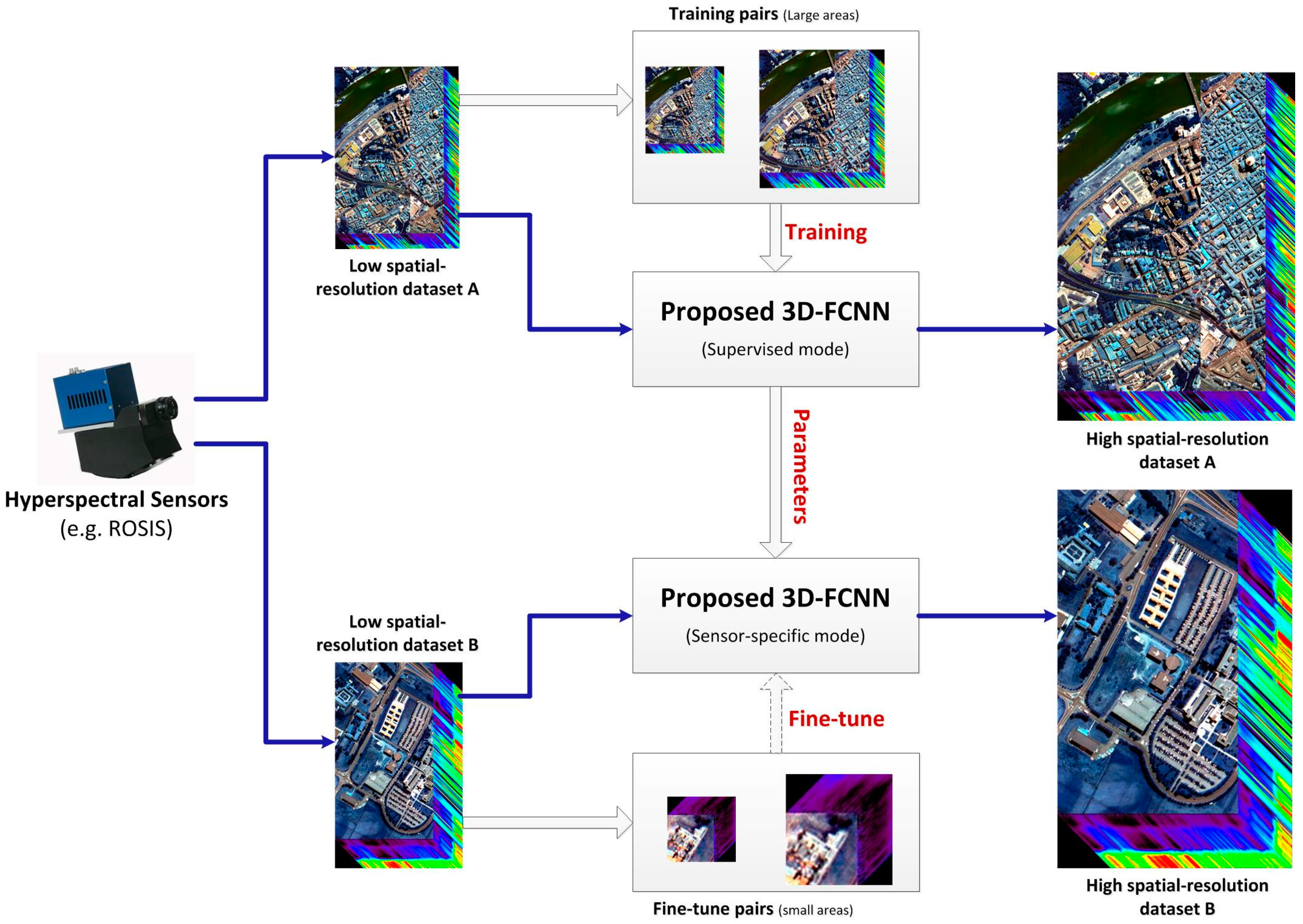
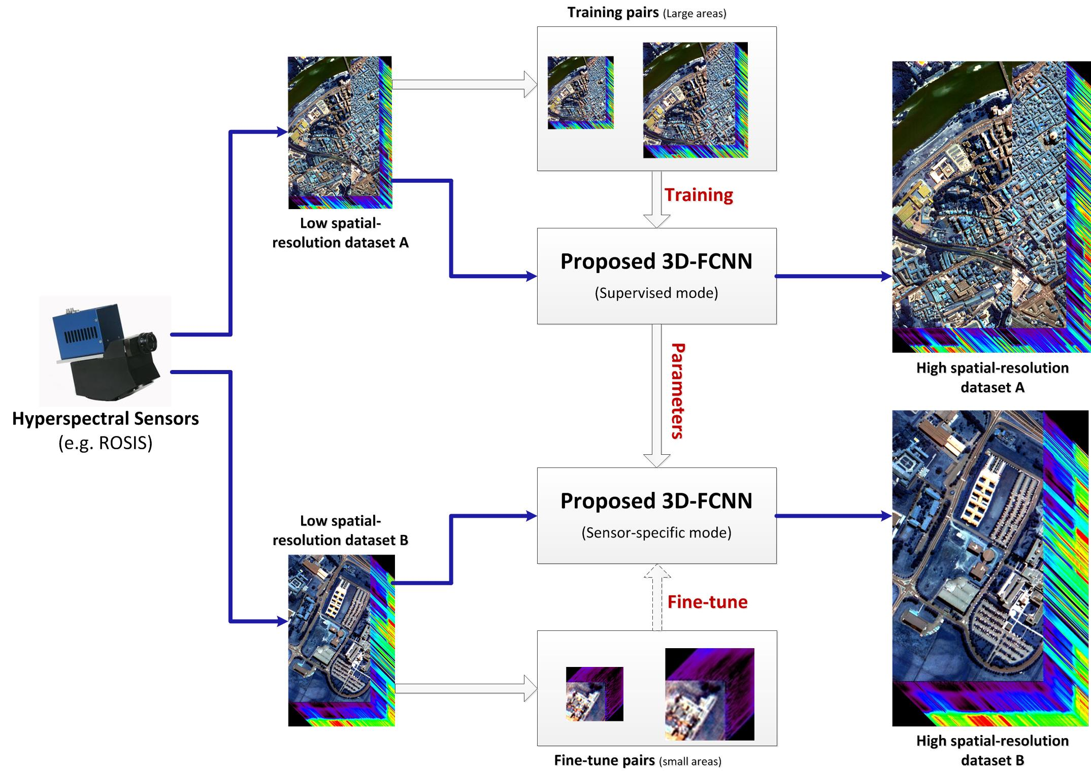
In this paper, 3D convolution is used to explore both spatial context and spectral correlation for spatial SR of HSIs. Consequently, a 3D full convolutional network (3D-FCNN) is proposed for single-image spatial SR of HSIs without any auxiliary information. In order to solve the problem of training deep NN in HSIs where it is very difficult to acquire a large amount of training samples, our proposed 3D-FCNN is extended to a sensor-specific manner such that it can be trained with hyperspectral datasets collected by the same sensor as the targeted dataset. As a result, the requirement of a large amount of training samples from the target scene is avoided. As shown in Figure 1, our work can be divided into the following steps: (1) Training: constructing, training and validating 3D-FCNN for SR of HSIs; (2) Testing: applying the trained network to a sensor-specific task. Specifically, the SR of an HSI can be fulfilled by using a 3D-FCNN trained by HSIs acquired with the same sensor without extra training. Moreover, when possible, such sensor-specific 3D-FCNN can be fine-tuned with only a few training data from the target HSIs to further improve the performance of SR.

Figure 1. Illustration of the proposed 3D-FCNN for SR of HSIs.

2.1. Proposed 3D-FCNN for Spatial SR of HSIs

2.1.1. 2D Convolution

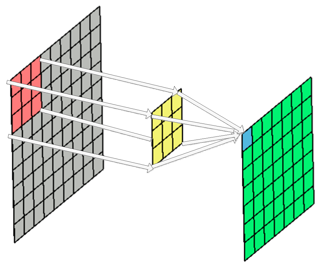
In a traditional 2D CNN, 2D convolution is performed to extract features from the previous layer. As shown in Figure 2, a convolution kernel is used to filter a small area of the image, so as to generate the feature value of these small regions. For each pixel of the image, the product of its neighboring pixels and the corresponding elements of the filter matrix is calculated and then added as the feature value of this pixel, which can be expressed as

$$c_{xy}=f\left({\displaystyle \sum _{i,j}{w}_{ij}{a}_{(x+i)\left(y+j\right)}+b}\right)$$

(1)

where $c_{xy}$ is the output feature value targeted at position $(x,y)$, $a_{(x+i)\left(y+j\right)}$ is the input unit at position $(x+i,y+j)$ with an offset of $\left(i,j\right)$ to $(x,y)$, $w_{ij}$ is the weight for the input $a_{(x+i)\left(y+j\right)}$ which is located at $\left(i,j\right)$ in the 2D convolution kernel, $b$ is the bias in the convolution neuron, and $f$ is the activation function. If the kernel has the size $F\times F$ and the input image has the size $W\times W$, the output feature map will have a smaller size $N\times N$, in which $N=W-F+1$.

Figure 2. Illustration of 2D convolution to extract spatial features.

In general, a convolution layer consists of a set of learnable filters (or kernels) that have small receptive fields, which are trained to learn specific types of features at the same spatial position in the input. In addition, parameters of kernel windows are forced to be identical to all possible locations of the previous layer, which is called weight sharing. Both the weight sharing technology and small receptive fields strategy can effectively reduce the number of parameters and increase the generalization capability of the network. Weights are replicated over the input image, leading to intrinsic insensitivity to translation in the input. A convolutional layer usually contains multiple feature maps so that multiple features can be detected. The network is trained with the back propagation (BP) gradient-descent procedure.

2.1.2. 3D Convolution

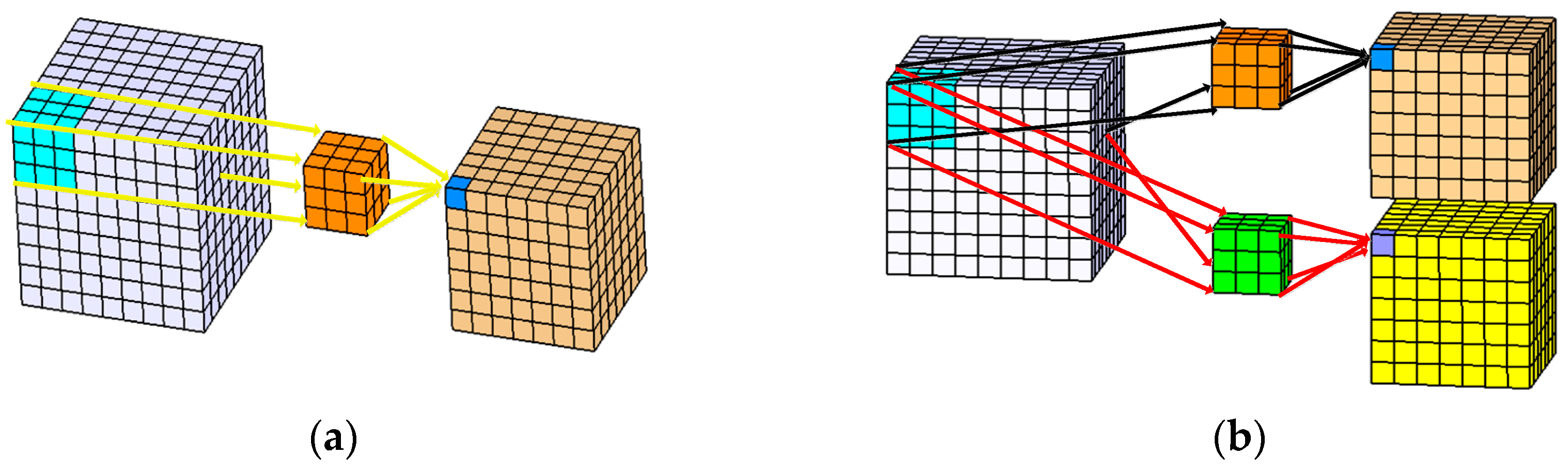
Though CNN has achieved great success in 2D convolution, the 2D convolution is only applied in the 2D space to capture spatial features. In 3D hyperspectral applications, the most straightforward method is to perform 2D CNN processing on each band of HSIs. However, such a 2D convolution on multiple images separately does not explore spectral information encoded in contiguous bands, easily resulting in spectral distortion. To this end, the spectral dimension should also be considered in the convolutional kernel to extract spectral features. Therefore, in this paper, 3D convolution instead of 2D convolution is used to simultaneously conduct convolution in both spatial and spectral dimensions to capture spatial-spectral features. As shown in Figure 3a, 3D convolution is realized by convolving a 3D kernel with the cube formed by stacking multiple contiguous spectral information together. By extending 2D convolution in Equation (1), 3D convolution is calculated as the weighted sum of pixels in a 3D data cube as

$$c_{xyz}=f\left({\displaystyle \sum _{i,j,k}{w}_{ijk}{a}_{(x+i)\left(y+j\right)(z+k)}+b}\right)$$

(2)

where $c_{xyz}$ is the output feature at position $(x,y,z)$, $a_{(x+i)\left(y+j\right)(z+k)}$ represents the input at the position $(x+i,y+j,z+k)$ in which $\left(i,j,k\right)$ denotes its offset to $(x,y,z)$, and $w_{ijk}$ is the weight for input a_{(x+i)(y+j)(z+k)} with an offset of $\left(i,j,k\right)$ in the 3D convolutional kernel. Similar to 2D convolution, the feature cube has a smaller size.

Figure 3. Illustration of 3D convolution: (a) illustration of a 3D kernel to extract spatial-spectral features; (b) illustration of multiple 3D kernels to extract different kinds of spatial-spectral local feature patterns.

Similar to the 2D convolution, weight sharing technique—in which the kernel weights are replicated across the entire cube—is also used in the 3D convolution such that one kernel extracts one type of feature all over the image cube. In order to explore different kinds of spatial-spectral local feature patterns, as shown in Figure 3b, multiple 3D convolutions with distinct kernels are applied to the same location in the previous layer.

2.1.3. The Architecture of the Proposed 3D-FCNN

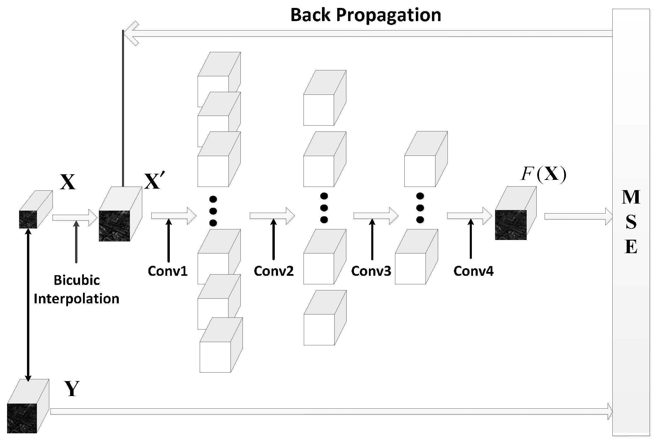
In this paper, as shown in Figure 4, a 3D-FCNN is constructed for SR of HSIs by using 3D convolution to fully explore spatial-spectral features in the 3D hyperspectral data cube. Considering a single-source low-resolution HSI $X$, it is firstly up-scaled to $X^{\prime }$ with the same size of desired output $Y$ using bicubic interpolation. Since only spatial information is taken into account in bicubic interpolation, 3D convolution is used to further improve the initial SR result $X^{\prime }$ by alleviating spectral distortion. Therefore, the initial SR result $X^{\prime }$ is entered into our 3D-FCNN to generate a high-spatial-resolution HSI $F(X)$ approaching the desired output $Y$ as accurately as possible, which can fully take advantages of both spatial context and spectral correlation.

Figure 4. Framework of the proposed 3D-FCNN for SR of HSIs.

The structure of our proposed 3D-FCNN is shown in Figure 4. It contains five layers including one input layer, and four convolutional layers where the output of the last convolutional layer is the output of the whole network. Generally, the number of parameters to be optimized is proportional to that of neurons in a CNN. In SR problems, the scale of the input, namely the initial super-resolution result $X^{\prime }$, heavily influences the scale of the network. In this paper, a sub-image, rather than the entire hyperspectral image, is fed to the 3D-FCNN. Specifically, as shown in Table 1, the input is restricted as a $33\times 33\times c\times 1$-pixel sub-image cube, where $33\times 33$ is spatial dimensions, $c$ is the special dimension depending on the sensor properties, and the color channel is set as 1 for HSIs. Therefore, all the filers in the successive convolution layers are designed to learn spectral information from $c$ contiguous spectral bands. It should be noted that larger sub-images can also be used as input to design the 3D-DCNN and its construction is similar to that in this paper. We restrict the network to a relatively small scale to be easily and quickly trained.

Table 1. Details of the proposed 3D-CNN for SR of HSIs.

Layer	Input Size	Kernel Size	Output Size
Conv1	$33\times 33\times c\times 1$	$9\times 9\times 7\times 64$	$25\times 25\times \left(c-6\right)\times 64$
Relu1	$25\times 25\times \left(c-6\right)\times 64$	-	$25\times 25\times \left(c-6\right)\times 64$
Conv2	$25\times 25\times \left(c-6\right)\times 64$	$1\times 1\times 1\times 32$	$25\times 25\times \left(c-6\right)\times 32$
Relu2	$25\times 25\times \left(c-6\right)\times 32$	-	$25\times 25\times \left(c-6\right)\times 32$
Conv3	$25\times 25\times \left(c-6\right)\times 32$	$1\times 1\times 1\times 9$	$25\times 25\times \left(c-6\right)\times 9$
Relu3	$25\times 25\times \left(c-6\right)\times 9$		$25\times 25\times \left(c-6\right)\times 9$
Conv4	$25\times 25\times \left(c-6\right)\times 9$	$5\times 5\times 3\times 1$	$21\times 21\times \left(c-8\right)\times 1$

As shown in Figure 4, four 3D convolutional layers are sequentially connected to the input layer to improve the performance of initial SR result by exploring both spatial context and spectral correlation. For the first three convolutional layers, the ‘ReLU’ function is adopted as activation function for nonlinear mapping since it improves models fitting without extra computational cost and over-fitting risk. Suppose the input of neurons in activation layers is represented as $I_i,i=1,2,\cdots$, their output is calculated in an element-wise manner as follows

$$O_i=\max \left\{I_i,0\right\},i=1,2,\dots$$

(3)

For the fourth convolutional layer, its output without the effect of activation function is used as the output of the whole network. The size of kernels in convolution layers is of crucial importance in CNN since it greatly affects the performance of the network. The size of different convolutional layers and ‘ReLU’ layers in our proposed 3D-FCNN are listed in Table 1.

According to Figure 4 and Table 1, in the proposed 3D-FCNN, 64 different 3D kernels with size $9\times 9\times 7$ ($9\times 9$ in spatial dimension and 7 in the spectral dimension) are conducted on the input data to generate 64 feature maps of the size $25\times 25\times \left(c-7+1\right)$ for Layer ‘Conv1’. Layer ‘Conv2’ consists of 32 features maps of the size $25\times 25\times \left(c-6\right)$, which are obtained by applying 32 different 3D kernels size of $1\times 1\times 1$ on the input of Conv1. The third convolution layer ‘Conv3’ is obtained by applying nine different 3D kernels of size $1\times 1\times 1$, resulting in nine feature maps with a size of $25\times 25\times \left(c-6\right)$. Finally, the output layer ‘Conv4’ applies a 3D kernel of the size $5\times 5\times 3$ to produce the output image $F(X)$ with size $21\times 21\times \left(c-8\right)$. In order to prevent the border effects that occur during training, all convolutions are not padding. Thus, as mentioned earlier, the actual output of the network is smaller than the input. Specifically, according to Table 1, the proposed 3D-FCNN uses an initial SR result of $33\times 33\times c$ to generate an image of $21\times 21\times \left(c-8\right)$.

Training an end-to-end network requires a cost function to optimize the parameters in the network. In practice, we use the mean squared error (MSE) between outputs and ground-truth as cost function. Considering the actual output of the network is a smaller image, MSE loss function is evaluated only by the difference between the central pixels of ground-truth high-resolution image $Y$ and the network output $F(X)$, which can be calculated as

$$MSE=\frac{1}{m}{\displaystyle \sum _{n=0}^m\left(\frac{1}{hwc}{\displaystyle \sum _{i=0}^h{\displaystyle \sum _{j=0}^w{\displaystyle \sum _{k=0}^c\left(Y_{ijk}-F{\left(X\right)}_{ijk}\right)}}}\right)}$$

(4)

where m is the number of training samples, h and w represent the length and width of the output of the network $F(X)$, respectively, and c is the band of the training samples. Generally, high Peak Signal to Noise Ratio (PSNR) can also be guaranteed by using MSE, which is widely used to evaluate image quality. Let n represent the number of bits per pixel. The PSNR can be calculated as

$$PSNR=10\times {\log }_{10}\left(\frac{{\left(2^n-1\right)}^2}{MSE}\right)$$

(5)

The loss function defined by Equation (4) is minimized using adaptive moment estimation (ADAM) with the standard BP algorithm, because it requires less memory, can calculate different adaptive learning rates for different parameters, and is suitable for large datasets and high dimensional space. The main advantage of ADAM is that the learning rate of each iteration has a definite range after the correction of bias, which makes the parameters more stable. In particular, the weight matrices are updated as

$$\begin{array}{l}{m}_t=\mu \times m_{t-1}+(1-\mu )\times g_t\\ n_t=v\times n_{t-1}+(1-v)\times g_t^2\\ {\widehat{m}}_t=\frac{m_t}{1-{\mu }^t}\\ {\widehat{n}}_t=\frac{n_t}{1-v^t}\\ \Delta {\theta }_t=-\frac{{\widehat{m}}_t}{\sqrt{{\widehat{n}}_t}+\epsilon }\times \eta \end{array}$$

(6)

where $t$ represents time-step, $g_t$ represents the gradients at time-step $t$, $m_t$ is the biased first moment estimate, $n_t$ is the biased second moment estimate, ${\widehat{m}}_t$ is the bias-corrected first moment estimate, ${\widehat{n}}_t$ is the bias-corrected second moment estimate, $\eta$ is the learning rate, ${\theta }_t$ is the parameter vector, and $\mu ,v\in \left[0,1\right)$ are exponential decay rates for the moment estimates.

2.2. Sensor-Specific Implementation

Our proposed 3D-FCNN can be extended to the spatial SR problem of hyperspectral sensors, such as ROSIS and HYDICE. Once the 3D-FCNN is well trained, its parameters can be used for a sensor-specific mission, which means that our trained network can be directly applied to different datasets obtained from the same sensor.

As shown in Figure 1, when the proposed 3D-FCNN is used for the sensor-specific mission, there are two modes as follows:

(1)

Unsupervised sensor-specific mode: the parameters involved in the network do not vary when being directly transferred to the target data obtained from the same sensor as the data trained on the proposed 3D-FCNN. As a result, any training data of the target dataset is not required. Thus, this network can be viewed as an unsupervised sensor-specific spatial SR system, which can be directly used for reconstructing high spatial-resolution HSI from the target low spatial-resolution HSI without changing the parameters of networks. In this mode, a large amount of training data and training time is avoided when it is used for the SR of the target scene. It should also be noted that such unsupervised sensor-specific mode is especially effective for the target scene which is acquired with similar imaging condition with the dataset on which the 3D-FCNN is trained.

(2)

Fine-tuning based sensor-specific mode: the parameters in the network trained under unsupervised sensor-specific mode can be further fine-tuned using the samples from the target dataset obtained by the same sensor. Through such fine-tuning, the performance of unsupervised sensor-specific spatial SR can be further improved. Such fine-tuning based sensor-specific mode is especially effective when the target scene is acquired with different imaging condition with the dataset on which the 3D-FCNN is trained. Only a small number of training samples is required, so the training based on sensor-specific initialization is very fast, compared with previous supervised training with random initialization.

3. Results

In this section, extensive experiments are conducted to verify the performance of the proposed 3D-FCNN for spatial SR of HSIs.

3.1. Datasets

Datasets from two well-known hyperspectral sensors, namely ROSIS and HYDICE, are used for evaluation. For the ROSIS sensor, two scenes that are acquired during a flight campaign over Pavia, northern Italy, i.e., Pavia Centre and Pavia University are selected. The Pavia Centre scene contains 1096 × 1096 pixels, while the Pavia University scene contains 610 × 340 pixels. In the Pavia Centre scene, samples that contain no information are discarded in this experiment and only 1096 × 715 valid pixels are used. The numbers of spectral bands are 102 for Pavia Centre and similarly 103 for Pavia University. For the HYDICE sensor, two datasets are adopted, namely the Washington DC Mall datasets and the Urban dataset. The Washington DC Mall datasets image contains 1280 × 307 pixels over 191 bands of the original 224 atmospherically corrected bands which are adopted by removing the channels associated with H₂O and OH absorption bands. The Urban HYDICE datasets is of size 307 × 307 and contains 210 atmospherically corrected bands.

These four datasets are used as ground-truth of high spatial-resolution HSIs to train and evaluate the performance of the proposed 3D-FCNN based framework for spatial SR. In order to simulate low spatial-resolution HSIs, these two images are firstly down-sampled using Gauss kernels. The size of sub-images used for training is set as $33\times 33\times c\times 1$, which is obtained by overlapping from the original dataset. The proposed 3D-FCNN based framework is designed, trained, and tested based on the Keras framework using the TensorFlow backend. The BP strategy is adopted to train the network. For the ADAM based training, the base learning rate is 0.00005.

3.2. Performance Evaluation

Many assessment methods have been used to evaluate the quality of a reconstructed hyperspectral image for SR and restoration [59]. In this experiment, the performance of SR for HSIs is evaluated by comparing the reconstructed high spatial-resolution HSI with the ground-truth data from two aspects: the spatial reconstruction quality of each band image at image levels and the spectral reconstruction quality of each spectrum at pixel-levels.

To evaluate the spatial reconstruction quality, the mean peak signal-to-noise ratio (MPSNR) and the mean structural similarity (MSSIM) index are adopted. The MPSNR is defined as

$$MPSNR=\frac{1}{c}{\displaystyle \sum _{i=0}^{c}10\times {\log }_{10}\left(\frac{MA{X_i}^2}{MS{E}_i}\right)}$$

(7)

where MAX_i is the maximal pixel value in the i-th band image, and $MS{E}_i$ is the $MSE$ of the i-th band image. The MSSIM between reconstructed image $F\left(X\right)$ and its ground truth $Y$ is defined as

$$MSSIM=\frac{1}{c}{\displaystyle \sum _{i=0}^c\frac{\left(2{\mu }_{F{\left(X\right)}_i}{\mu }_{Y_i}+c_1\right)\left(2{\sigma }_{F{\left(X\right)}_i{Y}_i}+c_2\right)}{\left({{\mu }^2}_{F{\left(X\right)}_i}+{{\mu }^2}_{Y_i}+c_1\right)\left({\sigma }_{F{(X)}_i}^2+{\sigma }_{Y_i}^2+c_2\right)}}$$

(8)

where $F{(X)}_i$ and $Y_i$ represents the i-th band image of $F\left(X\right)$ and $Y$, respectively, ${\mu }_{F{\left(X\right)}_i}$ and ${\mu }_{Y_i}$ are the mean of $F{(X)}_i$ and $Y_i$, respectively, ${\sigma }_{F{(X)}_i}^2$ and ${\sigma }_{Y_i}^2$ are the variance of $F{(X)}_i$ and $Y_i$, respectively, ${\sigma }_{F{\left(X\right)}_i{Y}_i}$ is the covariance of $F{(X)}_i$ and $Y_i$, and $c_1$ and $c_2$ are constants that are set as 0.0001 and 0.0009, respectively.

In order to evaluate the spectral reconstruction quality, the spectral angle mapper (SAM) between the reconstructed spectra and their corresponding ground-truth spectra is used. The SAM between two spectra $z$ and $z^{\prime }$ is defined as

$$SAM=\arccos \left(\frac{⟨z,z^{\prime }⟩}{{\Vert z\Vert }_2{\Vert z^{\prime }\Vert }_2}\right)$$

(9)

where $⟨z,z^{\prime }⟩$ represents the dot product of $z$ and $z^{\prime }$, and $\Vert {•\Vert }_2$ represents 2-norm of vectors.

Generally, a higher MPSNR and MSSIM value means a better visual quality, and a lower SAM value implies less spectral distortion and a higher quality of spectral reconstruction.

3.3. Experimental Results on Hyperspectral Datasets Acquired by ROSIS Sensor

Two datasets acquired by ROSIS sensor, namely Pavia Centre dataset and Pavia University dataset, were used to evaluate the performance of the proposed 3D-FCNN for SR. These two datasets are complemented to 103 bands by setting the missing bands as 0.

3.3.1. Experimental Results of Spatial SR with the Proposed 3D-FCNN Method

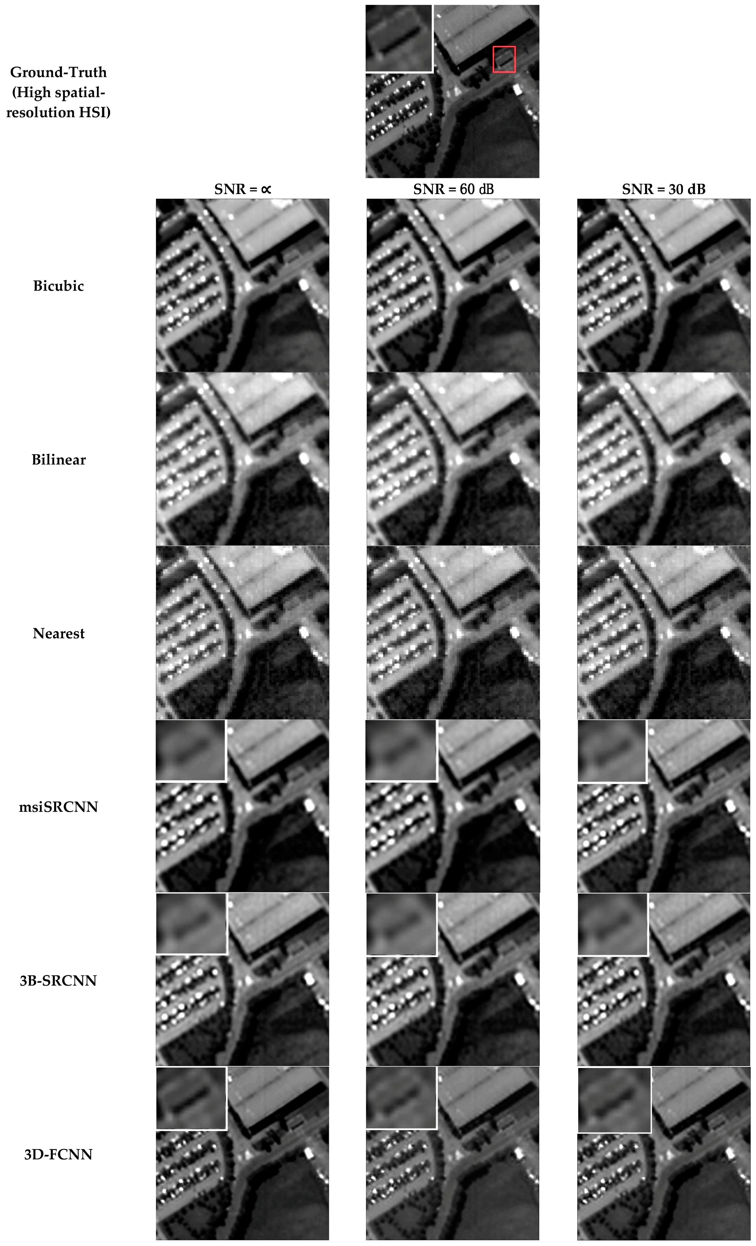
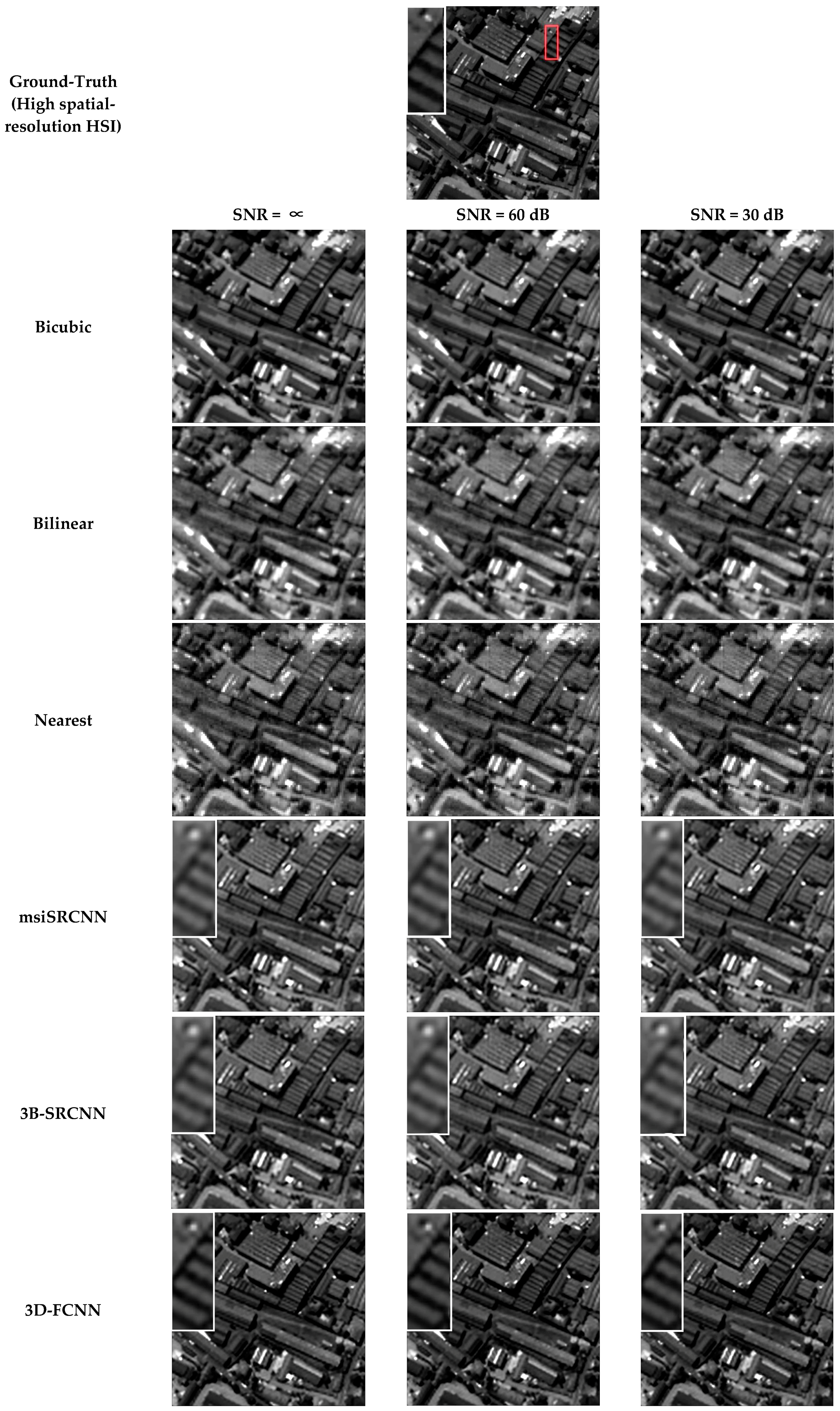
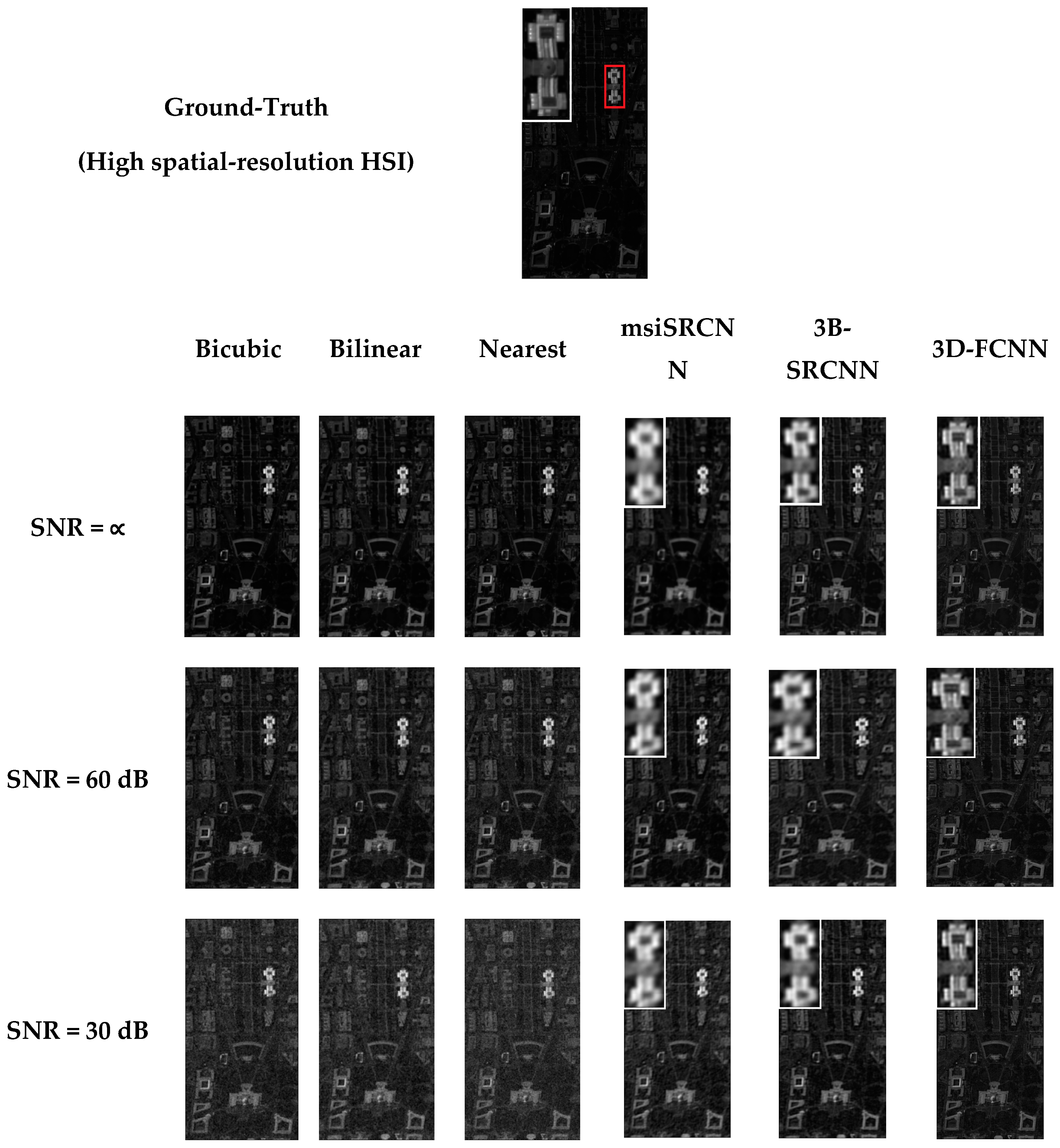
The performance of the proposed 3D-FCNN for spatial SR is evaluated over the two selected datasets. For each dataset, a $150\times 150$ sub-region is selected to validate the performance of our proposed 3D-FCNN, while the remaining pixels are used for training. In order to simulate low spatial-resolution HSIs, these two images are firstly down-sampled by a factor of 2. In addition, different levels of additive Gaussian white noise, measured by signal-to-noise ratio (SNR), are added to the low spatial-resolution images to verify the robustness of the proposed 3D-FCNN to noises.

Five strategies are chosen as the baseline for comparison: Bicubic SR, Bilinear SR, SR by nearest neighbor, SRCNN [40,42] in a band-by-band manner (namely misSRCNN in [44]) and three-band-wise manner (denoted as 3B-SRCNN). The qualitative comparison results of all the considered algorithms are listed in Table 2. Their corresponding visual results are shown in Figure 5 and Figure 6, respectively. It is also observed that: (1) the proposed 3D-FCNN obviously outperforms all the other algorithms all over these two datasets by ROSIS sensor with the highest MPSNR and MSSIM values and lowest SAM for all the cases; (2) The proposed 3D-FCNN provides better results no matter how noisy the dataset is. The average improvements in MPSNR are 2.572 dB and 2.878 dB, and in MSSIM are 0.033 and 0.032 compared with Bicubic when $SNR=30$ dB and $SNR=60$ dB, respectively, indicating that the proposed 3D-FCNN is robust to noises in low spatial-resolution HSI; (3) The proposed 3D-FCNN based algorithm provides much better spectral fidelity (i.e., lower SAM) compared with SRCNN (msiSRCNN and 3B-SRCNN). 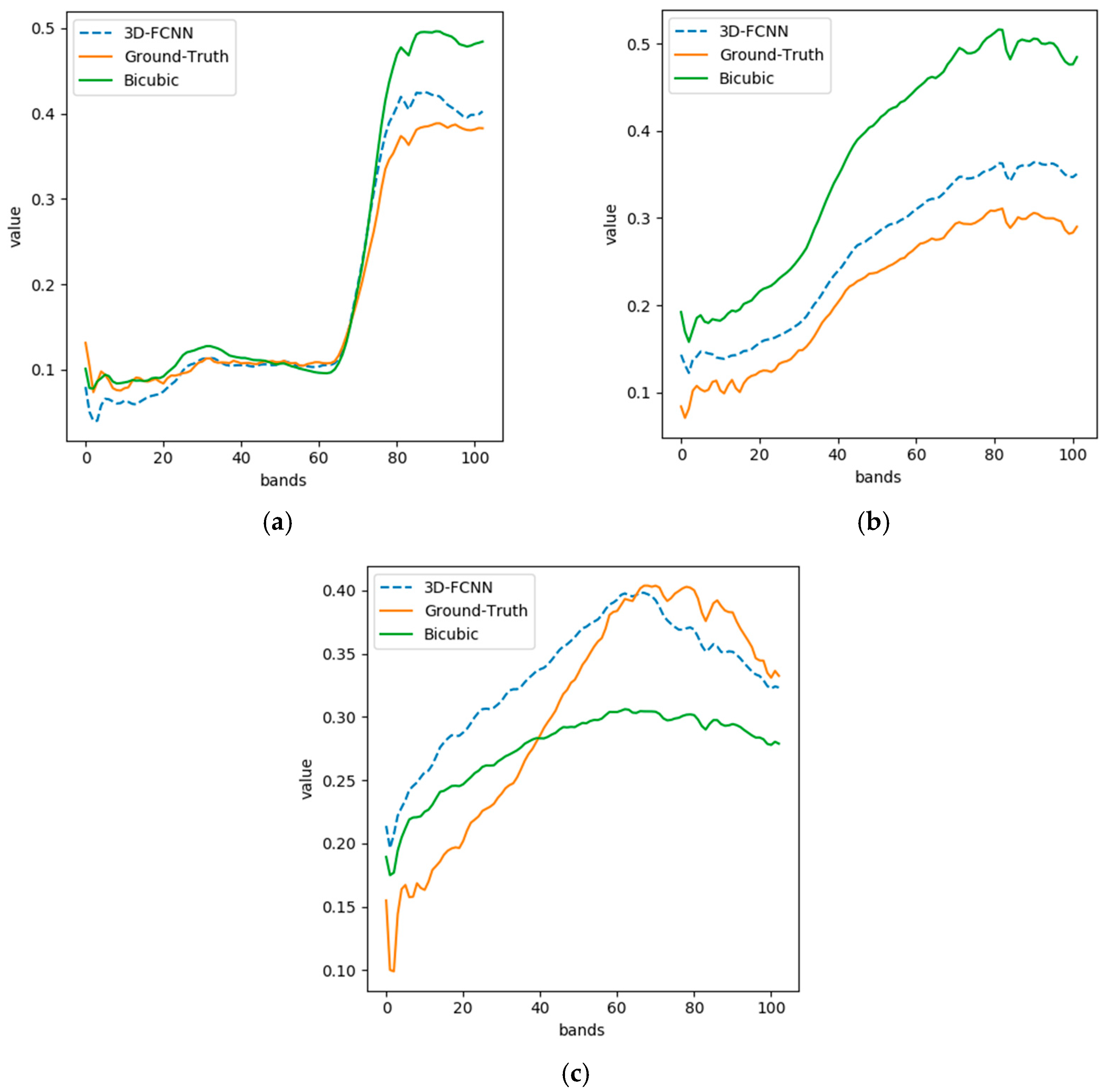Figure 7 further lists the spectra of several typical ground materials after spatial SR. It can be observed that the spectra reconstructed by the proposed 3D-FCNN is closer to their ground-truth than that by the bicubic spatial interpolation, demonstrating that the proposed 3D-FCNN can better maintain spectral characteristics during spatial SR. This is because both spatial context in neighboring areas and spectral correlation in full-band images are considered in the proposed method by 3D convolution; (4) The proposed 3D-FCNN based algorithm also achieves best spatial reconstruction for all the cases, which has the highest MPSNR and MSSIM values. Compared with the Bicubic algorithm, the average improvements are 2.849 dB in terms of MPSNR and 0.035 for MSSIM.

Table 2. Quantitative comparison results of different SR methods on HSIs by ROSIS sensor.

	SNR (dB)		Bicubic	Bilinear	Nearest	msiSRCNN	3B-SRCNN	3D-FCNN
Pavia Centre	$\infty$	MPSNR	31.1	29.909	29.983	32.479	32.686	33.916
		MSSIM	0.937	0.915	0.921	0.957	0.96	0.969
		SAM	4.592	5.009	4.786	4.617	4.661	4.14
	60	MPSNR	31.097	29.907	29.979	32.238	32.746	33.97
		MSSIM	0.937	0.915	0.921	0.955	0.96	0.969
		SAM	4.606	5.019	4.805	4.765	4.693	4.163
	30	MPSNR	31.083	29.9	29.966	32.248	32.762	33.86
		MSSIM	0.937	0.914	0.921	0.955	0.96	0.968
		SAM	4.606	5.046	4.86	4.793	4.687	4.218
Pavia University	$\infty$	MPSNR	29.499	28.599	28.752	29.253	30.083	32.381
		MSSIM	0.925	0.906	0.914	0.923	0.936	0.964
		SAM	3.946	4.38	4.243	4.197	4.071	3.454
	60	MPSNR	29.495	28.597	28.748	29.096	30.13	31.701
		MSSIM	0.925	0.906	0.914	0.92	0.939	0.958
		SAM	3.965	4.391	4.267	4.323	4.041	3.807
	30	MPSNR	29.484	28.591	28.736	29.173	29.898	31.852
		MSSIM	0.925	0.906	0.913	0.921	0.935	0.958
		SAM	4.018	4.425	4.333	4.335	4.142	3.778

Figure 5. The visual results of spatial SR on the Pavia Centre dataset, in which the area in the red rectangle is enlarged in the upper left corner of the image.

Figure 6. The visual results of spatial SR on the Pavia University dataset, in which the area in the red rectangle is enlarged in the upper left corner of the image.

Figure 7. Example spectra of several typical materials in this image scene: (a) trees; (b) meadows; and (c) asphalt.

3.3.2. Experimental Results of SR for Different Up-Sampling Factors

In this subsection, the SR results of different up-sampling factors are discussed. The low spatial-resolution HSIs are simulated by down-sampling the high spatial-resolution HSI with the factor 2, 3 and 4, respectively. Then different SR algorithms are used for spatial SR. Similar to previous experiments, only a $150\times 150$ sub-region from the Pavia Centre datasets is used for validation of the performance of our proposed 3D-FCNN, while all the remaining areas are used for training. Table 3 lists the quantitative results by different SR algorithms for different up-sampling factors over the Pavia Centre area. It is observed that, the performance of our proposed 3D-FCNN outperforms all the other algorithms with different up-sampling factors. When the up-sampling factor increases, the superiority of our proposed 3D-FCNN becomes less obvious. This is because the problem of SR with a higher up-sampling factor is more difficult. However, even for 4 times spatial SR, the proposed 3D-FCNN achieves an improvement of 1.74 in MPSNR, 0.045 in MSSIM, and 0.287 in SAM, respectively, compared with the Bicubic method.

Table 3. Quantitative comparison of spatial SR for different up-sampling factors over the Pavia Centre dataset.

			Bicubic	Bilinear	Nearest	msiSRCNN	3B-SRCNN	3D-FCNN
Pavia Centre	$n=2$	MPSNR	31.1	29.909	29.983	32.479	32.686	33.916
		MSSIM	0.937	0.915	0.921	0.957	0.96	0.969
		SAM	4.592	5.009	4.786	4.617	4.661	4.14
	$n=3$	MPSNR	28.519	27.907	27.57	29.159	29.261	29.853
		MSSIM	0.882	0.859	0.857	0.889	0.905	0.921
		SAM	5.571	5.85	5.864	5.49	5.376	5.300
	$n=4$	MPSNR	26.83	26.327	26.21	26.21	27.256	27.59
		MSSIM	0.808	0.783	0.792	0.792	0.851	0.862
		SAM	6.362	6.694	6.616	6.616	6.404	6.336

$n$ is the factor of up-sampling.

3.3.3. Experimental Results of Sensor-Specific SR by the Proposed 3D-FCNN

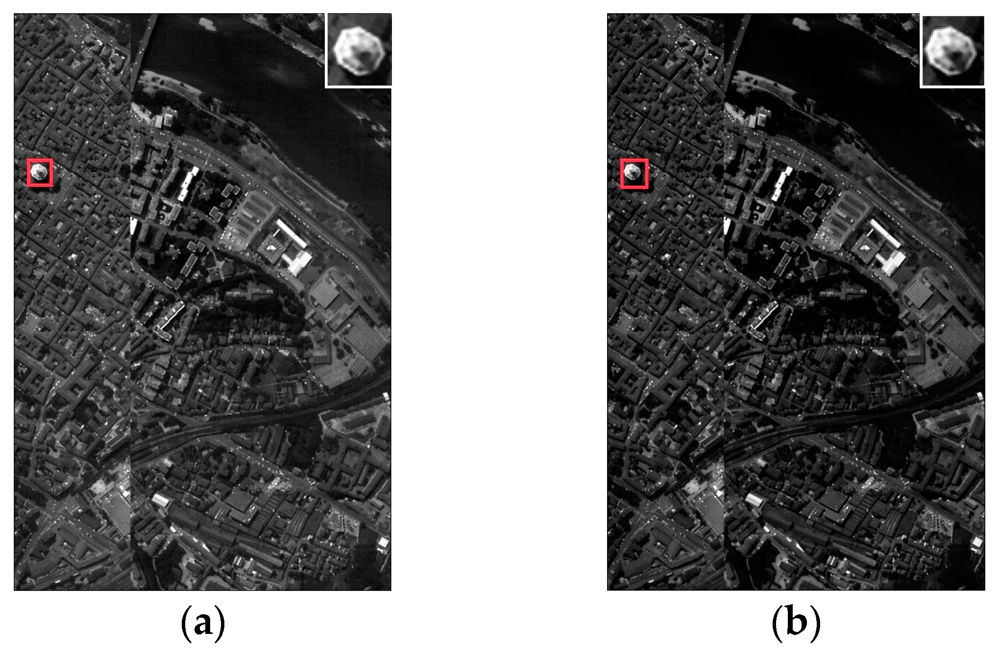
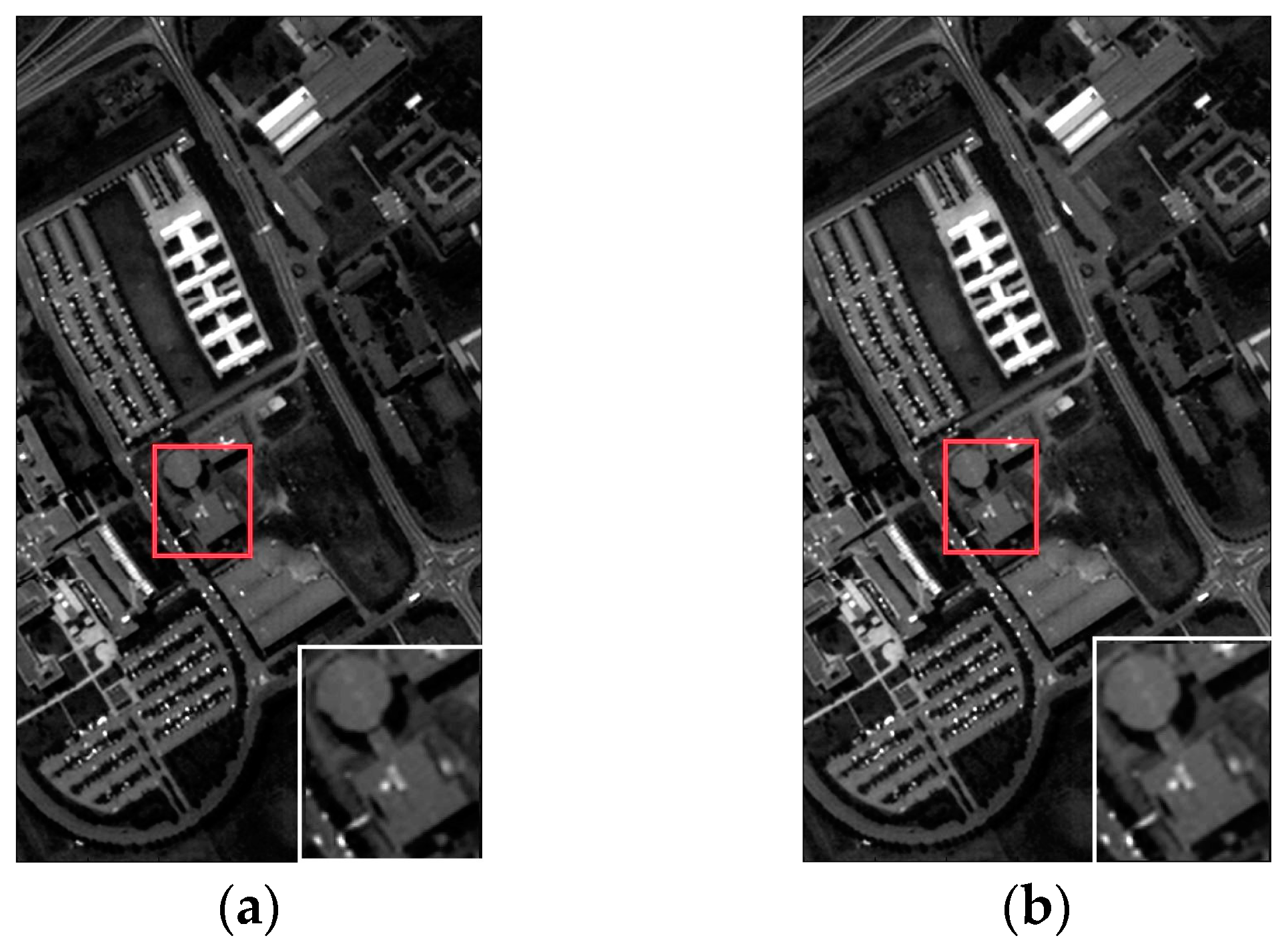
In this experiment, the 3D-FCNN is used for spatial SR of HSIs in a sensor-specific manner, which means that it is trained on one dataset and directly applied for spatial SR of other datasets acquired by the same sensor without any tuning of parameters. Specifically, the 3D-FCNN trained on the Pavia Centre dataset is used for spatial SR of the Pavia University dataset, and the model trained on the Pavia University dataset is used for spatial SR of the Pavia Centre dataset. Such sensor-specific manner can be viewed as an unsupervised version of our proposed 3D-FCNN for spatial SR of HSIs since training samples from the target scene are not required. In addition, the performance of fine-tuning for sensor-specific SR, in which the parameters of sensor-specific 3D-FCNN is fine-tuned with a limited number of available training samples from target datasets, is also tested.

Table 4 lists the quantitative results from our proposed 3D-FCNN for spatial SR of the two datasets from the ROSIS sensor. The results of previous supervised 3D-FCNN are also listed as benchmark results. It is observed that, the performance of spatial SR by the proposed 3D-FCNN does not degrade even if it is not trained by the targeted datasets, demonstrating the effectiveness of the proposed sensor-specific strategy for spatial SR of hyperspectral sensors. The visual results of our proposed 3D-FCNN for spatial SR of the Pavia Centre dataset and the Pavia University dataset are shown in Figure 8 and Figure 9, respectively, including both supervised mode that is trained by samples from the target scene and sensor-specific mode that is trained by other datasets from the same sensor. These results also confirmed that our proposed sensor-specific mode is very effective for spatial SR of HSIs. However, it avoids the requirement of a huge amount of training samples from the target scene and the time-consuming training.

Table 4. Quantitative comparative results of the proposed 3D-FCNN for SR of datasets from the ROSIS sensor in different modes.

		Supervised	Sensor-Specific	Fine-Tune
				50	100	150
Pavia Centre	MPSNR	34.908	34.899	34.937	34.978	34.998
	MSSIM	0.979	0.979	0.977	0.979	0.979
	SAM	4.396	4.447	4.429	4.423	4.424
		Supervised	Sensor-Specific	Fine-Tune
				50	100	150
Pavia University	MPSNR	34.519	34.506	34.49	34.502	34.559
	MSSIM	0.977	0.977	0.976	0.976	0.976
	SAM	3.16	3.172	3.168	3.146	3.122

50, 100, 150 is the number of fine-tuning samples.

Figure 8. Visual results of spatial SR for the Pavia Centre dataset by the proposed 3D-FCNN: (a) supervised mode by training the network using samples from the Pavia Centre dataset; (b) sensor-specific mode by training the network using sample from the ROSIS sensor, i.e., the Pavia University dataset. The area in the red rectangle is enlarged in the upper left corner of the image.

Figure 9. Visual results of spatial SR for the Pavia University dataset by the proposed 3D-FCNN: (a) supervised mode by training the network using samples from the Pavia University dataset; (b) sensor-specific mode by training the network using sample from the ROSIS sensor, i.e., the Pavia Centre dataset. The area in the red rectangle is enlarged in the lower right corner of the image.

It is also observed from Table 4 that the fine-tuning process of training sensor-specific 3D-FCNN with a few samples from the target dataset cannot improve the performance of sensor-specific very much. This may be because these two datasets are acquired during one flight and the imaging condition, e.g., acquisition time, weather, atmosphere, texture of images, etc., does not vary much. Therefore, we further evaluated the performance of our proposed 3D-FCNN on two datasets acquired at different imaging conditions by the HYDICE sensor.

3.4. Experiments on Hyperspectral Datasets Acquired by the HYDICE Sensor

Two datasets acquired by the HYDICE sensor, namely the Washington DC Mall and Urban datasets, are used to evaluate the performance of the proposed 3D-FCNN. As with the ROSISI sensor, the two datasets are complemented to 210 bands by setting the missing bands as 0.

3.4.1. Experimental Results of SR with the Proposed 3D-FCNN Method

Since the Urban dataset is too small to train the proposed 3D-FCNN, only the Washington DC Mall dataset is selected to evaluate the performance of the proposed 3D-FCNN for SR in supervised mode. Unlike the ROSIS sensor, we selected a larger region with 600 × 307 pixels to test the performance of our proposed 3D-FCNN, while the remaining pixels are used for training. The image is firstly down-sampled by a factor of 2 and additive Gaussian white noises are added to the simulated low-dimensional HSI such that the robustness of the 3D-FCNN is tested for images with different SNRs. Five strategies are chosen as the baseline for comparison: Bicubic SR, Bilinear SR, SR by nearest neighbor, SRCNN [40,42] in a band-by-band manner (namely misSRCNN in [44]) and three-band-wise manner (denoted as 3B-SRCNN).

The qualitative comparison results of all the considered algorithms are listed in Table 5. These results also confirm similar conclusions from previous experiments: (1) the performance of our 3D-FCNN obviously outperforms traditional methods, i.e., Bicubic SR, Bilinear SR and SR by nearest neighbor; (2) the spectral distortion caused by applying SRCNN of natural images directly to HSIs in band-wise manner or 3-band-group manner can be greatly alleviated by the 3D convolution in the proposed 3D-FCNN algorithm; (3) the proposed 3D-FCNN is robust to noise. Even in very noisy cases when $SNR=30$ dB, our proposed 3D-FCNN improves the performance of 3B-FCNN (the second best results) by about 2.5 dB in MPSNR, 0.02 in MSSIM, and 0.2 in SAM. The visual results of all these algorithms are also listed in Figure 10, which demonstrate the superiority of the proposed 3D-FCNN for spatial SR of HSIs.

Table 5. Quantitative results of different methods for spatial SR of the Washington DC Mall dataset.

	SNR(dB)		Bicubic	Bilinear	Nearest	msiSRCNN	3B-SRCNN	3D-FCNN
Washington DC Mall	$\infty$	MPSNR	47.588	46.76	46.89	45.866	49.62	53.556
		MSSIM	0.981	0.979	0.98	0.956	0.976	0.989
		SAM	0.455	0.49	0.462	0.718	0.56	0.357
	60	MPSNR	42.503	41.876	41.465	42.929	43.908	46.028
		MSSIM	0.978	0.975	0.973	0.966	0.971	0.987
		SAM	0.544	0.564	0.602	0.647	0.614	0.412
	30	MPSNR	39.004	38.713	37.924	40.94	41.743	44.288
		MSSIM	0.963	0.965	0.954	0.96	0.968	0.984
		SAM	0.749	0.711	0.844	0.735	0.668	0.481

Figure 10. The spatial SR results of the Washington DC Mall dataset for low-dimensional images with different SNRs. The results of msiSRCNN, 3B-SRCNN and the proposed 3D-FCNN are enlarged in the upper left corner.

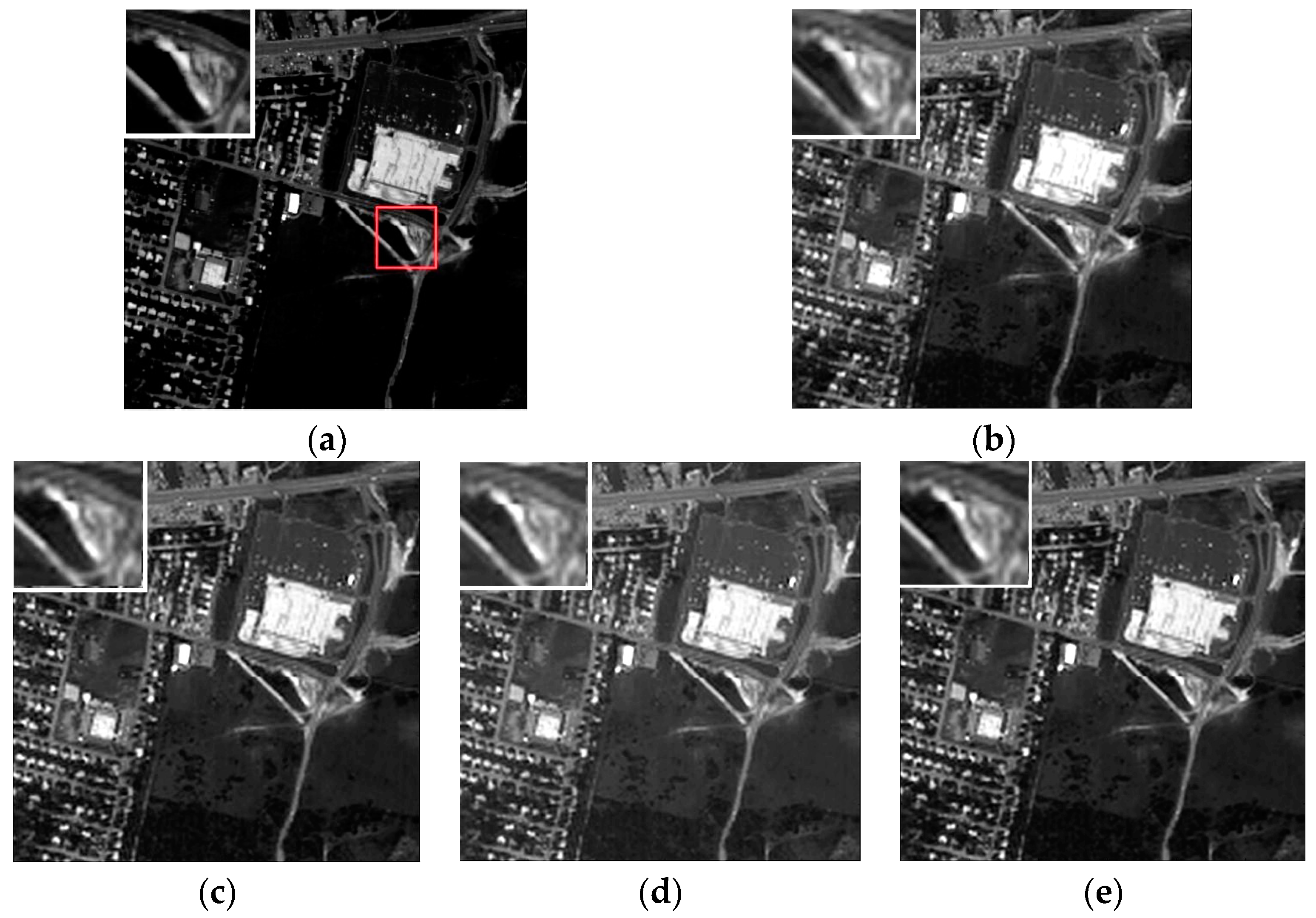
3.4.2. Experimental Results of Sensor Specific SR for the HYDICE Sensor

In this experiment, the 3D-FCNN trained on the Washington DC Mall dataset is directly applied for spatial SR of the Urban dataset in a sensor-specific manner. The performance of fine-tuning is also tested. The spatial SR results of the Urban dataset using sensor-specific 3D-FCNN are listed in Table 6. It is observed that the performance of sensor-specific 3D-FCNN can be effectively improved by the fine-tuning process, especially for the quality of spectral reconstruction. When more training samples from the target scene are used for fine-tuning, slightly better results can be achieved. This is because these two datasets are acquired under different conditions, i.e., different time, weather, atmosphere, etc. As shown in these results, the performance of sensor-specific spatial SR can be further improved when even a small amount of training samples from the target scene is used for fine-tuning. These conclusions are also confirmed by the visual results listed in Figure 11.

Table 6. Quantitative results of the proposed 3D-FCNN for sensor-specific spatial SR.

		Sensor-Specific	Fine-Tune
			50	100	150
Urban	MPSNR	27.563	28.922	29.039	29.091
	MSSIM	0.89	0.93	0.932	0.933
	SAM	14.04	11.67	11.525	11.457

50, 100, 150 is the number of fine-tuning samples.

Figure 11. Visual results of spatial SR over the Urban dataset. (a) Ground-Truth (High spatial-resolution HSI); (b) Sensor-specific SR; (c) Fine-tuning with 50 samples; (d) Fine-tuning with 100 samples; (e) Fine-tuning with 150 samples.

4. Discussion

The 3D-FCNN is proposed to learn an end-to-end full-band mapping between low and high spatial-resolution HSIs. It can effectively reconstruct high spatial-resolution HSI using a single low spatial-resolution HSI without any auxiliary information. According to previous experiments, its sensor-specific version can restore a high spatial-resolution HSI without the requirement of training on it. Generally, fine-tuning by using training samples from the target scene can improve the performance of SR. However, if the target scene is acquired with similar conditions to the scene that the 3D-FCNN is trained over, there is no need to fine-tune the network for SR since the performance of SR cannot be further improved.

Table 7 lists the computation time of three CNN based spatial SR algorithms for the Pavia Centre dataset by the ROSIS sensor. All these algorithms are implemented on a computer with one GPU card (NVIDI GTX1070 with 16GB memory). It is observed that, in order to learn the spectral correlation in adjacent band images, our proposed 3D-FCNN takes more time for training. However, once our network is well trained, it takes less than one second to reconstruct an image, indicating that it is computationally effective when working under an unsupervised sensor-specific manner.

Table 7. The computation time of different SR methods on the Pavia Centre dataset.

	msiSRCNN	3B-SRCNN	3D-FCNN
Training	7 h	9 h	20 h
Test	0.492 s	0.536 s	0.426 s

In order to further evaluate the performance of our proposed 3D-FCNN with different parameters for SR, various experiments are conducted over the Pavia University dataset by varying different parameters involved in the proposed 3D-FCNN, including the number of convolutional layers, the size of input, activation function, filter size, and the size of receptive field. The corresponding results are listed in Table 8, Table 9, Table 10, Table 11 and Table 12.

Table 8. Experimental results of the proposed 3D-FCNN with different numbers of convolutional layers over the Pavia University datasets while other parameters are fixed as listed in Table 1.

Number of 3D Convonlution Layers	MPSNR	SAM
3	33.64	4.27
4	33.92	4.14
5	33.78	4.19
6	33.70	4.29

Table 9. Experimental results of the proposed 3D-FCNN with different sizes of input over the Pavia University datasets while other parameters are fixed as listed in Table 1.

Size of Input	MPSNR	SAM
33 × 33 × c	33.92	4.14
44 × 44 × c	33.84	4.21
55 × 55 × c	33.79	4.25

Table 10. Experimental results of the proposed 3D-FCNN with different activation functions over the Pavia University datasets while other parameters are fixed as listed in Table 1.

Activation Function	MPSNR	SAM
Relu	33.92	4.14
Tanh	33.37	4.19
PRelu	33.76	4.29

Table 11. Experimental results of the proposed 3D-FCNN with different filter sizes over the Pavia University datasets while other parameters are fixed as listed in Table 1.

Filter Size	MPSNR	SAM
64-32-9-1	33.92	4.14
64-32-16-1	33.85	4.17
32-16-8-1	33.67	4.24

Table 12. Experimental results of the proposed 3D-FCNN with different sizes of receptive field over the Pavia University datasets while other parameters are fixed as listed in Table 1.

Receptive Field	MPSNR	SAM	Parameters
12	33.92	4.14	39403
14	33.94	4.13	55789
16	34.03	4.11	88557

As shown in Table 8, the 3D-FCNN with four convolutional layers slightly outperforms that with other numbers of convolutional layers. Actually, the 3D-FCNN with different convolutional layers does not vary much. Here, four convolutional layers are adopted since more convolutional layers will bring about many more parameters to be learned and the computational time for training and testing will increase rapidly.

In Table 9, the 3D-FCNN with the input of 33x33xc slightly outperforms that with other inputs. Moreover, larger inputs also result in more parameters to be trained.

The 3D-FCNN with the activation function of ‘Relu’ slightly outperforms the other two well-known activation functions, namely ‘Tanh’ and ‘PRelu’, as tabulated in Table 10.

In terms of the filter size, as shown in Table 11, the 3D-FCNN with ‘64-32-9-1’ slightly outperforms that with other filters, where the numbers in these filters represent the last dimension of filters listed in ‘Table 1’ (in the manuscript) for the four convolutional layers, respectively.

As for the size of receptive field in Table 12, the 3D-FCNN with a receptive field of 16 produces the best results. However, the number of parameters are much more than that with a smaller receptive field. Therefore, 12 is adopted to achieve the balance between the performance of SR and computational complexity.

5. Conclusions and Future Work

In this paper, a novel 3D-FCNN model is proposed for spatial SR of HSIs by learning an end-to-end full-band mapping between low and high spatial-resolution HSIs. Compared with traditional CNN based SR algorithms in color images, 3D convolution is used to reconstruct a high spatial-resolution HSI by exploring both spatial context in neighboring areas and spectral correlation in neighboring bands, such that the spectral distortion can be alleviated. The proposed 3D-FCNN is also extended to a sensor-specific version such that well-trained 3D-FCNN from a dataset can be directly used for spatial SR of other HSIs from the same sensor. The training samples from the target scene, if available, can also be used to further improve the performance of sensor-specific spatial SR. Experiments on four simulated datasets by two well-known hyperspectral sensors have demonstrated the proposed 3D-FCNN based spatial SR algorithm obviously outperforms existing methods and it is also very effective to reconstruct sensor-specific spatial SR which is more practically useful.

Recent work in SR of HSIs proposed to use CNN for SR of spectral difference of HSIs [44,45]. The proposed 3D-FCNN can also be extended for this kind of SR. In addition, using 3D-FCNN for SR of HSIs in both spatial and spectral domains is also of interest for future research.