Predicting Top-of-Atmosphere Thermal Radiance Using MERRA-2 Atmospheric Data with Deep Learning ^†

Abstract

Image data from space-borne thermal infrared (IR) sensors are used for a variety of applications, however they are often limited by their temporal resolution (i.e., repeat coverage). To potentially increase the temporal availability of thermal image data, a study was performed to determine the extent to which thermal image data can be simulated from available atmospheric and surface data. The work conducted here explored the use of Modern-Era Retrospective analysis for Research and Applications, Version 2 (MERRA-2) developed by The National Aeronautics and Space Administration (NASA) to predict top-of-atmosphere (TOA) thermal IR radiance globally at time scales finer than available satellite data. For this case study, TOA radiance data was derived for band 31 (10.97 $\mathsf{\mu }$m) of the Moderate-Resolution Imaging Spectroradiometer (MODIS) sensor. Two approaches have been followed, namely an atmospheric radiative transfer forward modeling approach and a supervised learning approach. The first approach uses forward modeling to predict TOA radiance from the available surface and atmospheric data. The second approach applied four different supervised learning algorithms to the atmospheric data. The algorithms included a linear least squares regression model, a non-linear support vector regression (SVR) model, a multi-layer perceptron (MLP), and a convolutional neural network (CNN). This research found that the multi-layer perceptron model produced the lowest overall error rates with an root mean square error (RMSE) of 1.36 W/m${}^2$·sr·$\mathsf{\mu }$m when compared to actual Terra/MODIS band 31 image data. These studies found that for radiances above 6 W/m${}^2$·sr·$\mathsf{\mu }$m, the forward modeling approach could predict TOA radiance to within 12 percent, and the best supervised learning approach can predict TOA to within 11 percent.

1. Introduction

Thermal infrared satellite data have been widely used for cross-calibration studies [1] and climate research [2,3]. However, thermal infrared satellites such as Landsat and Terra/Moderate-Resolution Imaging Spectroradiometer (MODIS) have limited temporal resolution (Landsat has a revisit rate of up to 16 days while Terra/MODIS has a revisit rate of 1–2 days). Thermal instruments on geostationary satellites (e.g., The Geostationary Operational Environmental Satellite system (GOES)) have much finer temporal resolution, but have large view angles through the atmosphere for a significant portion of the disk, limiting their utility for cross-calibration. Atmospheric reanalysis data is available on a global spatial grid at three hour time intervals and could potentially be utilized to derive top-of-atmosphere (TOA) thermal radiance data at timescales that are finer than current satellite data. Higher temporal resolution could open the door to new applications and enable more detailed study of temporally localized climate phenomena.

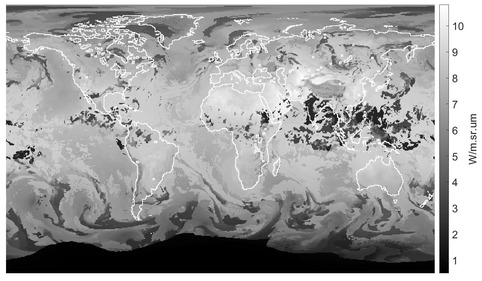
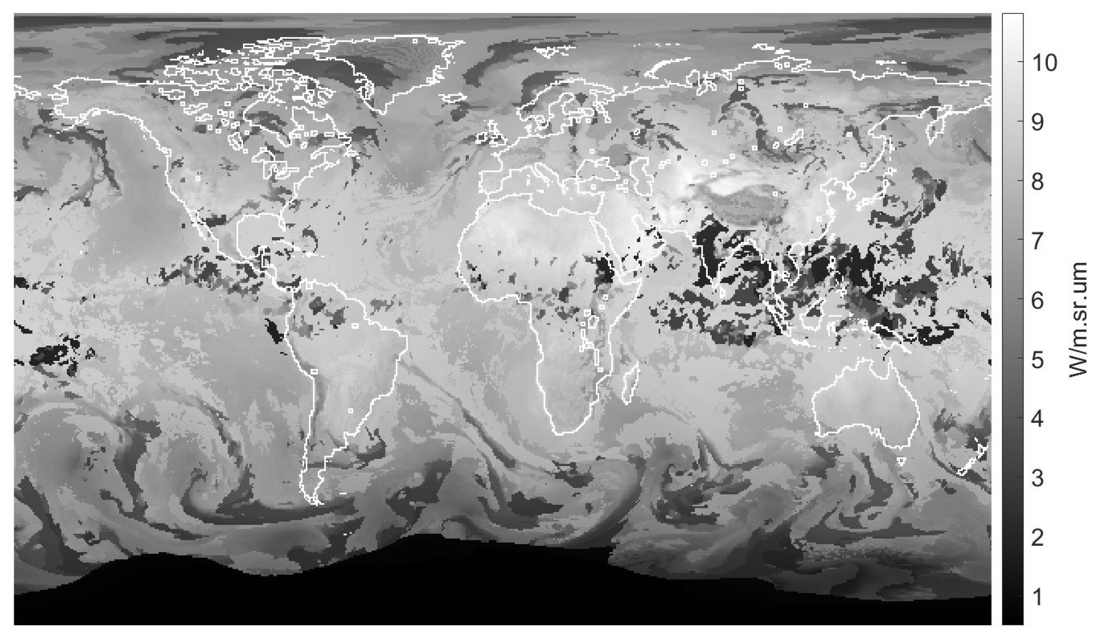
This paper describes an approach to predicting TOA thermal infrared radiance using the Modern-Era Retrospective analysis for Research and Applications, Version 2 (MERRA-2) reanalysis data product (See Figure 1). Atmospheric reanalysis data have been used in research to account for atmospheric effects [4] and calibration studies [5]. A recent study has used MERRA-2 atmospheric data together with Landsat [6] radiance data to predict surface temperature, but no studies have used MERRA-2 to predict TOA radiance.

The central goal of this paper is to assess the feasibility of using the MERRA-2 data products with supervised machine learning algorithms to derive TOA radiance in the same spectral band as band 31 of the MODIS sensor. Note that MODIS band 31 is used here as an example space-based IR sensor, but the techniques may be applied to other similar sensors. Broadly, this paper uses two approaches for predicting TOA thermal radiance from MERRA-2: (1) an atmospheric radiative transfer forward modeling approach and (2) supervised machine learning. The first approach calculated TOA radiance by using the MERRA-2 atmospheric data as input to the MODerate resolution atmospheric TRANsmission (MODTRAN) [7] atmospheric radiative transfer model. For the second approach, four regression techniques were used for predicting TOA thermal infrared radiance from MERRA-2 air temperature, relative humidity, and skin temperature data as well as emissivity data from the Advanced Spaceborne Thermal Emission and Reflection Radiometer Global Emissivity Database (ASTER-GED). The first technique was linear least squares, and the second was a non-linear support vector regression (SVR) model. The remaining two regression models were deep artificial neural networks (ANNs). Since 2013, interest in deep ANNs (i.e., deep learning) has grown enormously in the field of machine learning due to their success at predicting and forecasting in various fields, and significant success has been reached with image classification [8], financial forecasting [9] and general regression problems [10]. These various approaches to predict TOA radiance are discussed here along with results and an assessment of the variables affecting the derived TOA radiance values. The two deep learning models used here were a multi-layer perceptron (MLP) and a convolutional neural network (CNN). These models learn how to hierarchically extract discriminative features for regression tasks. A detailed description of all regression models is given in Section 3.

A preliminary version of these results with the non-deep learning models has been previously published [11]. The results in this paper are significantly improved and a larger test set is used.

2. Data

All models used MERRA-2 atmospheric data (i.e., air temperature profiles, relative humidity profiles, skin temperature) along with emissivity from the ASTER Global Emissivity Dataset as input. Terra/MODIS band 31, the MODIS cloud mask (MOD 35) and the MODIS land cover maps (to indicate water or land) were used for model validation and error analysis.

2.1. MERRA-2

The Global Modeling and Assimilation Office developed MERRA-2 as an Earth System reanalysis product [12]. It provides worldwide atmospheric measurements dating from 1980 to the present. The global coverage, along with its continuous three-hourly data record, is where MERRA-2’s strength lies. Depending on the application, the low spatial resolution of 0.5 × 0.625 degrees, which corresponds to about 50 km in the latitudinal direction, could be a limiting factor. Data from MERRA-2 has been used for a variety of climate research and renewable energy studies (e.g., [13,14,15]).

MERRA-2 consists of 42 collections (e.g., assimilated meteorological fields, surface flux diagnostics) containing multiple variables each (e.g., relative humidity, skin temperature). All variables are represented on a global grid of $576\times 361$ values (i.e., spatial locations in the world). Some variables have an atmospheric profile represented by multiple layers. For example, the air temperature variable can be interpreted as a $576\times 361\times 42$ data cube, where the 42 indicates 42 respective pressure levels interpolated from 72 vertical levels. 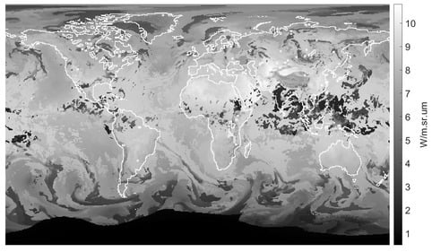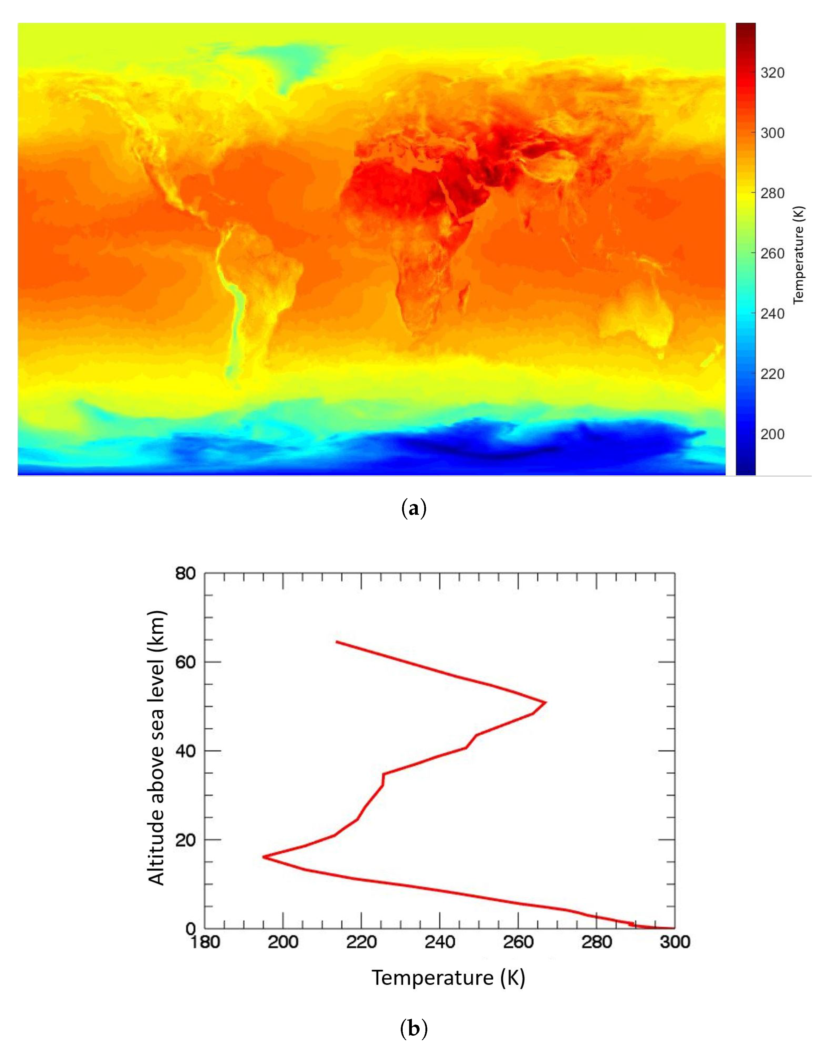Figure 2a displays the skin temperature global grid for 31 July 2013 at 08:55 Greenwich Mean Time (GMT). Figure 2b displays one air temperature profile against the altitude in kilometers above sea level that corresponds to the associated pressure levels. Four MERRA-2 variables were used for this paper: (1) instantaneous skin temperature (TS); (2) time-averaged skin temperature (TSH); (3) air temperature (T); and (4) relative humidity (RH). The air temperature and relative humidity variables are found in the “Assimilated Meteorological Fields” collection (inst3_3d_asm_Np) [16], while the surface skin temperature is found in the “Single-Level Diagnostics” collection (inst1_2d_asm_Nx) [17] and effective surface skin temperature is found in the “Surface Flux Diagnostics” collection (tavg1_2d_flx_Nx) [18]. The air temperature and relative humidity variables are assimilated using radar and satellite observations as well as conventional observations (e.g., radiosondes, dropsondes, aircraft, and global positioning system (GPS) radio occultation profiles [19]).

The instantaneous skin temperature collection is available hourly. Time-averaged skin temperatures are available at 00:30 GMT, 01:30 GMT, 02:30 GMT, etc. Relative humidity and air temperature variables are available every three hours starting at 00:00 GMT. The time-averaged skin temperature was linearly interpolated to coincide with the same three hour periods as the relative humidity and air temperature variables.

Where land is above sea level, all MERRA-2 variables with an atmospheric profile have no data below that atmospheric level. MERRA-2 encodes these variables using a numeric data type value representing an undefined (NaN) values. The supervised regression models cannot interpret NaNs, and they must be changed. Common strategies in machine learning are to swap them out for some other value. In this work, NaNs were replaced with zeros, which is a common strategy.

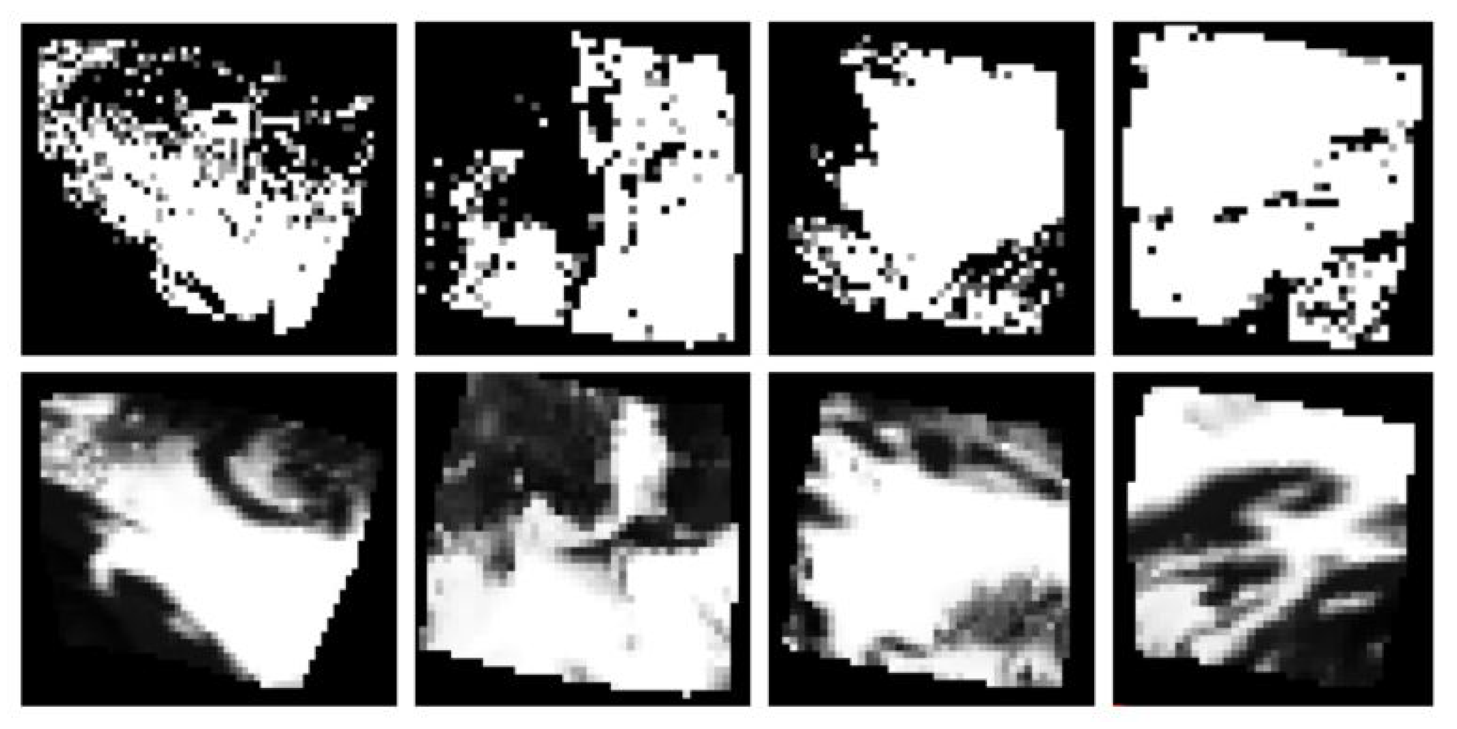
Two other MERRA-2 variables that were investigated for the prediction of TOA thermal infrared radiance were the 2D and 3D total cloud area fraction variable (from the Aerosol and Cloud Diagnostics collections) with continuous values between zero and one. Visual comparison between the MODIS cloud mask and the MERRA-2 2D total cloud area fraction variable suggested that the MERRA-2 cloud area fraction variable would not improve model performance. Figure 3 displays cloud masks for four of the test scenes. The top row displays MODIS cloud masks, while the bottom row displays the coincident MERRA-2 total cloud area fraction variables. Significant differences are visible between clouds (darker pixels) in the MODIS cloud mask and coincident MERRA-2 cloud area fraction variable. The 3D cloud area fraction variable was included and tested in one multi-layer perceptron model, but did not improve model results. Therefore these variables were not included in the models described in Section 3.

2.2. MODIS

All models were evaluated using the Moderate-Resolution Imaging Spectroradiometer (MODIS) [20] on-board the Terra satellite, v6. MODIS repeatedly views regions of the Earth’s surface every 1 to 2 days. Its thermal bands have a spatial resolution of 1 km at nadir. Twelve Terra/MODIS thermal infrared radiance scenes were used for reference data. Terra/MODIS thermal data band 31 (with range from 10.78 to 11.28 $\mathsf{\mu }$m) was used as a reference since it is well calibrated [21] with a calibration uncertainly of less than 0.13%.

The MODIS global land cover map (with a spatial resolution of $0.0833$ degrees) was used to indicate land or water. The land cover classification map is generated using the System for Terrestrial Ecosystem Parameterization (STEP) database as training data for the MCD12Q1 product algorithm [22].

The MODIS cloud mask (MOD35_L2), containing data collected from the Terra platform, is produced as an Earth Observing System (EOS) standard product. The cloud mask product consists of information regarding surface obstruction and various ancillary information affecting surface and cloud retrievals such as sun glint, land/water flag and non-terrain shadows. To determine if a cloud was present, only pixels indicating cloudy were used.

2.3. ASTER Global Emissivity Database

Temporally coincident monthly emissivity maps were selected from the Advanced Spaceborne Thermal Emission and Reflection Radiometer Global Emissivity Database (ASTER GED) [23]. The ASTER GED was created by processing millions of items of cloud-free ASTER data and calculating an average emissivity of the surface at approx 100 m and 1 km spatial resolution at the five ASTER Thermal Infrared (TIR) wavelengths. The 11.3 $\mathsf{\mu }$m wavelength was used for this paper since its is the closest to the Terra/MODIS band 31 band center of 10.97 $\mathsf{\mu }$m.

3. Methods

Five models were evaluated for predicting TOA thermal radiance from MERRA-2 atmospheric data. While four of the models used machine learning methods to perform a regression between the MERRA-2 input and the MODIS output for a training set, a radiative transfer model was also applied as a baseline to compare the supervised models against. The first three models are briefly described, namely the atmospheric radiative transfer model (ARTM), linear regression model (LR) and support vector regression (SVR). Following this, the deep learning models are described in detail. This paper assumes limited prior knowledge of supervised machine learning or deep learning.

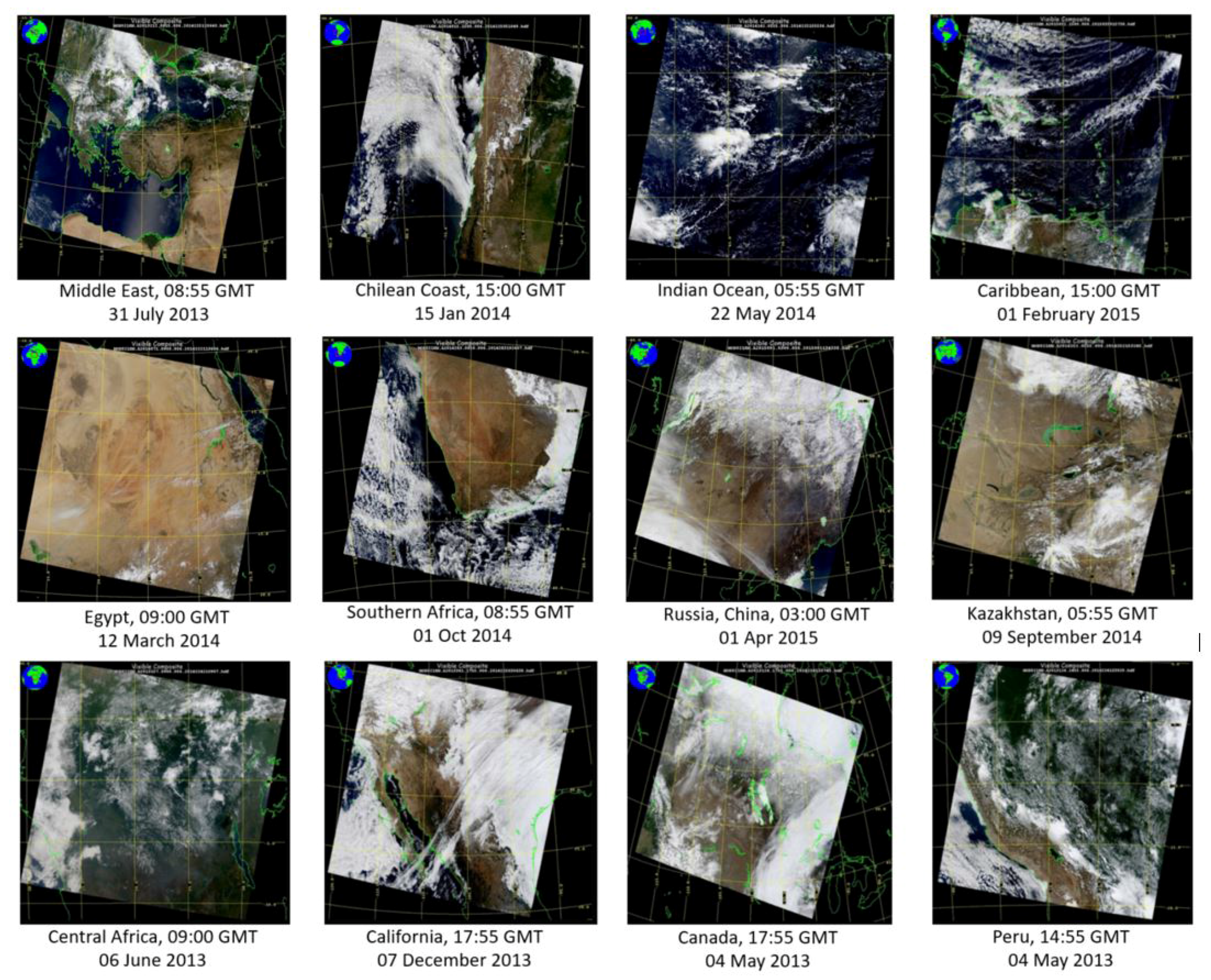
Twelve Terra/MODIS band 31 test scenes were chosen to coincide temporally with the three-hourly air temperature and relative humidity fields in MERRA-2, and for their diverse cloud and land cover. Each scene was bi-linearly down-sampled to the same spatial resolution as MERRA-2 data (0.5 × 0.625 degrees) and georegistered onto their respective predicted TOA radiance maps. Figure 4 displays the Terra/MODIS test scenes (in true-color) that were used for evaluating all models. The location and date of each scene is displayed below each image. The training set, which contains none of the scenes in the test set, has scenes from all seasons, various cloud covers, and a variety of land cover (i.e., barren or sparsely vegetated, croplands, evergreen and deciduous forests, open shrublands, and the Pacific, Indian, Atlantic, and Mediterranean oceans). All data used for testing and training models ranged in date between 2013 and 2015.

3.1. Atmospheric Radiative Transfer Model

Generally, if surface temperature and emissivity are known and atmospheric profile data (e.g., radiosonde data) are available, sensor reaching thermal radiance can be estimated using an atmospheric radiative transfer model. The first method of calculating TOA radiance involved using MERRA-2 atmospheric parameters directly as input to MODTRAN. To specify the atmospheric profile, air temperature and dew point temperature profiles are needed. Since relative humidity is the ratio of how much moisture is in the atmosphere to how much moisture the atmosphere could hold at that temperature, the dew point was calculated using the MERRA-2 air temperature and the relative humidity variables.

The lowest air temperature value of each MERRA-2 air temperature profile was replaced with the coincident skin temperature variable before entering the profiles into MODTRAN, along with the dew point profiles and emissivity. MODTRAN simulations were run for wavelengths between $10.540$ microns and $11.536$ microns to coincide with the MODIS band 31 relative spectral response (RSR). The band-effective radiance was calculated by:

$$L=\frac{\int L_{\lambda }R\left(\lambda \right)d\lambda }{\int R\left(\lambda \right)d\lambda }\left[\frac{\mathrm{W}}{{\mathrm{m}}^2\mathrm{sr}\mathsf{\mu }\mathrm{m}}\right]$$

(1)

where $L_{\lambda }$ is the spectral radiance reaching the sensor, and $R\left(\lambda \right)$ is the MODIS band 31 normalized spectral response function.

3.2. Supervised Learning Models

For supervised regression models, it is necessary to fit the parameters (training) to data that are disjointed from the data used to evaluate them. The training set consisted of 38 temporally and spatially coincident Terra/MODIS and MERRA-2 scenes. At the MERRA-2 spatial resolution this led to 11,255 training instances, of which a random $10\%$ was used for validating the deep learning models (i.e., tuning hyper-parameters). Reference data (training labels) consisted of the down-sampled Terra/MODIS band 31 radiance pixel values. Only data within a 20-degree field of view (FOV) of the MODIS scene center were used to minimize atmospheric view-angle effects [24]. Models were validated by applying the trained models to 3539 disjoint test instances (not part of the training or validation set). These test instances were taken from the same twelve Terra/MODIS test scenes used in the atmospheric radiative transfer model. To speed up the training of the supervised learning models, various training instance lengths were examined. This was reduced by using less atmospheric layers from the air temperature and relative humidity fields. Experiments based on using a different number of levels showed that using the first 27 atmospheric layers from 1000 hPa to 50 hPa (corresponding to 0 km to approx. 21 km above sea level) produced better results than using data from all 42 levels, which is expected given that water vapor is the main influence at thermal IR wavelengths and most of the atmospheric water vapor is below 20 km.

3.2.1. Least Squares Linear Regression

The first machine learning approach used to estimate TOA thermal radiance was a least squares linear regression model, which serves as a simple baseline model for assessing the relative performance of the other methods. This regression model is given by

$$\widehat{y}={\mathbf{w}}^T\mathbf{x}+b,$$

(2)

where $\mathbf{x}$ is the input (i.e., MERRA-2 temperatures and relative humidity variables), b and $\mathbf{w}$ are parameters (or weights) learned from training data, and $\widehat{y}$ is the predicted TOA thermal radiance. Note that the bias (or intercept) term b can be incorporated into $\mathbf{w}$ by simply appending a ‘1’ to $\mathbf{x}$. The parameters are estimated by minimizing the expected error between the Terra/MODIS TOA thermal radiance reference data and the predicted radiance values over the complete training set:

$$\widehat{\mathbf{w}}=\underset{\mathbf{w}}{argmin}\sum _{i=1}^n\left({\left(y_i-{\mathbf{w}}^T{\mathbf{x}}_i\right)}^2+\alpha {\parallel \mathbf{w}\parallel }_2^2\right),$$

(3)

where n is the total number of $({\mathbf{x}}_i,y_i)$ training data points and ${\alpha \parallel \mathbf{w}\parallel }_2$ incorporates L2 (ridge) regularization to prevent overfitting, with $\alpha$ controlling the strength of the regularization [25]. For simplicity, in Equation (3), the bias term b has been incorporated into $\mathbf{w}$. This optimization can be solved analytically using the Moore–Penrose pseudo-inverse. Data used in this model was not normalized, thus all variables were left unchanged (i.e., temperature variables (K) and relative humidity values between zero and one).

3.2.2. Non-Linear Support Vector Regression

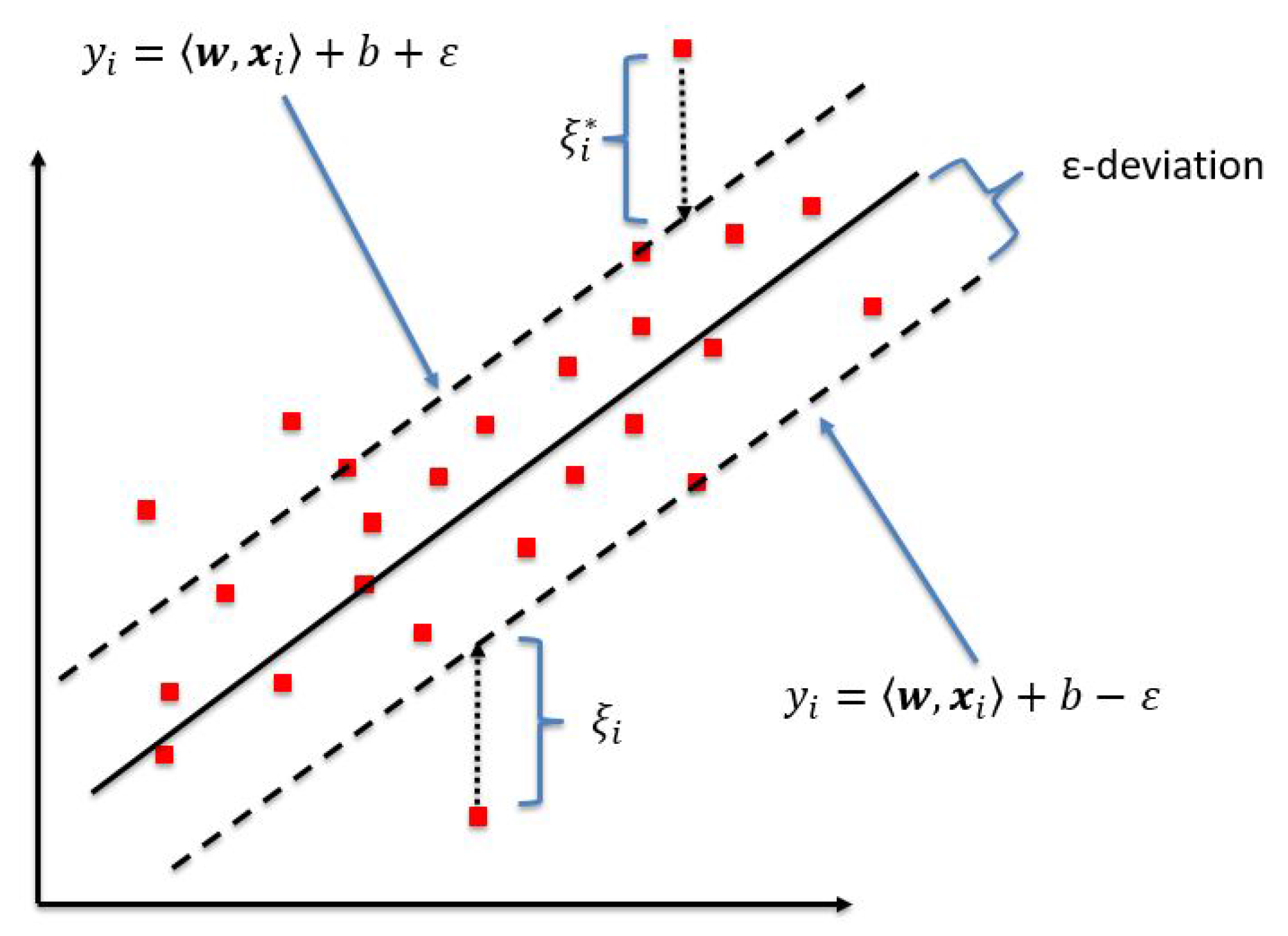
SVR [26] is an extension of the support vector machine (SVM) to regression problems, and it can make more complex predictions than the linear regression model. A one-dimensional example of SVR is shown in Figure 5, where the data points represent the predicted values $\left(\widehat{y}\right)$ and the line represents the truth/reference/label $\left(y\right)$ data. The two dashed lines are the bounds that are $ϵ$ distance away from the reference data, where $ϵ$ is a parameter chosen by the user. SVR uses only values outside the dashed lines to build the model. Training an SVR means solving:

$$\mathrm{minimize}\frac{1}{2}{\left|\right|\mathbf{w}\left|\right|}^2+C\sum _{i=1}^n({\xi }_i^{*}+{\xi }_i)$$

(4)

$$\mathrm{subject}\mathrm{to}\left\{\begin{array}{c}{y}_i-〈\mathbf{w},{\mathbf{x}}_i〉-b\le ϵ+{\xi }_i^{*}\hfill \\ 〈\mathbf{w},{\mathbf{x}}_i〉+b-y_i\le ϵ+{\xi }_i\hfill \end{array}\right.$$

where $\mathbf{w}$ is the learned weight vector, ${\mathbf{x}}_i$ is the i-th training instance, $y_i$ is the training label, and ${\xi }_i$ the distance between the bounds and predicted values outside the bounds. C is another parameter set by the user that is a constraint that controls the penalty imposed on observations outside the bounds that helps to prevent overfitting.

To make the model capable of non-linear predictions, every dot/inner product $〈\mathbf{w},{\mathbf{x}}_i〉$ is replaced by a radial basis function (RBF) kernel to map the data to a higher dimensional feature space. Without the use of a kernel (i.e., linear SVR), the main difference between it and linear regression is that SVR uses only a subset of the data, ignoring the points close to the model’s prediction, and SVR’s optimization does not depend on the dimensionality of the input space. The machine learning toolbox scikit-learn [27] implementation was used for the calculations.

Training and test data sets were the same as used in the linear regression model. Because of the distance calculation performed by the RBF kernel, the input features needed to be scaled to the same interval. Therefore, the data was normalized by dividing all temperature variables by the global maximum temperature, so that all training variables ranged in values between zero and one.

3.2.3. Multi-Layer Perceptron

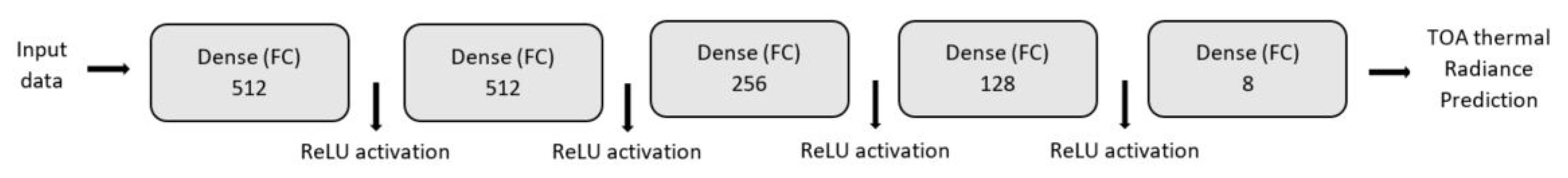
While linear regression can only model linear functions, artificial neural networks (ANNs) are universal function approximators [28]. A feedforward multi-layer perceptron (MLP) ANN consists of an input layer (i.e., the input variables), hidden layer(s), and an output layer. Each layer has a number of units (or neurons) within it, and these have learnable parameters (weights). Formally, the five-layer neural network model used here is given by:

$$\widehat{y}=\sigma \left({\mathbf{w}}^T\sigma \left(b_5+{\mathbf{H}}_5^T\sigma \left(b_4+{\mathbf{H}}_4^T\sigma \left(b_3+{\mathbf{H}}_3^T\sigma \left(b_2+{\mathbf{H}}_2^T\sigma \left(b_1+{\mathbf{H}}_1^T\mathbf{x}\right)\right)\right)\right)\right)\right),$$

(5)

where ${\mathbf{H}}_j$ are matrices containing the parameters for the hidden layers (the columns contain the weights for each unit), $b_j$ are the bias parameters, $\mathbf{x}$ is the input, and $\sigma \left(·\right)$ is an ‘activation’ function that is applied element-wise, which enables the model to make non-linear predictions.

If all hidden layers and activation functions are identity functions, then the MLP will be identical to the linear regression model. The rectified linear unit (ReLU) activation function [29], $\sigma \left(v\right)=max\left(v,0\right)$ was used, which sets all negative values to zero. ReLU is simple and tends to work significantly better than sigmoidal activation functions, and it was one of the innovations that enabled deep neural networks. Figure 6 displays a schematic of the network architecture indicating the size of each fully connected layer.

To find values for the MLPs parameters that produce a good fit to the training data, the error between the model’s predictions and the training data must be minimized, which is described by a loss function. However, unlike SVR and linear regression, it is not possible to find the global minima, but a local optima can be found using error backpropagation. To do this with the MLP model, mean squared loss was minimized. The initial learning rate used with backpropagation (to find how much to update the weights in the direction to decrease the gradient) of 0.001 was reduced ($\times 0.1$) when the validation loss did not decrease for five consecutive epochs (iteration of going through the whole dataset). Each training instance consisted of the air temperature and relative humidity profiles, instantaneous and time-averaged skin temperatures, and the emissivity variable. To train and run the network, Keras [30] with the Theano [31] back-end was used in Python.

3.2.4. Convolutional Neural Network

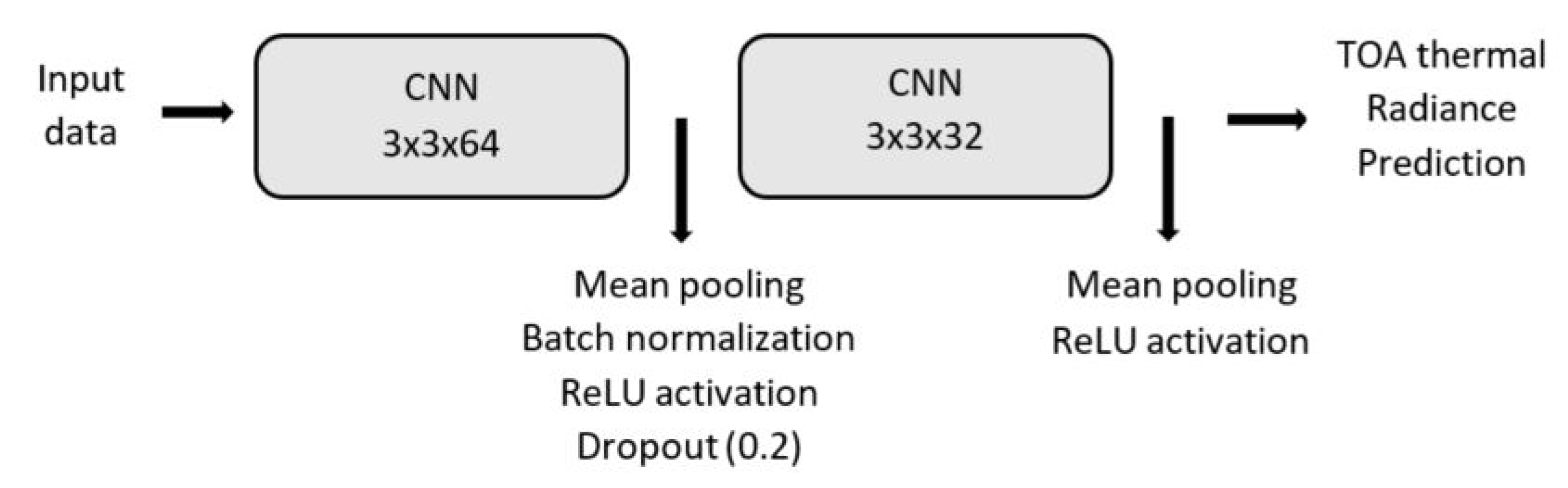
MLP’s do not explicitly encode spatial information, i.e., the features neighboring a particular latitude/longitude are ignored. The neighborhood information may improve the model’s ability to make predictions. Convolutional neural networks (CNNs) are capable of including neighboring spatial information in a computationally efficient manner. A CNN is similar to an MLP. However, the hidden units are replaced by learnable filters that are convolved with the input from the previous layer. The training and test instances for the CNN were created using a $9\times 9$ window around the spatial location of interest.

The CNN model, shown in Figure 7, consisted of only two convolutional layers, and then a fully-connected output layer. After each hidden layer, the output was down-sampled with mean pooling, reducing it’s dimensionality. Two regularization techniques were used to prevent overfitting: batch normalization [32] and drop-out [33]. Both were applied only after the first convolutional layer for both models.

More convolutional layers added to the second CNN did not improve the model in preliminary experiments.

4. Results

All models were evaluated using the twelve down-sampled MODIS band 31 thermal test scenes as described in Section 3. Root mean square error (RMSE), standard deviation, and mean error were used to evaluate model performance, along with percent error evaluations divided into radiance bins. All error metrics are reported in W/m${}^2$·sr·$\mathsf{\mu }$m.

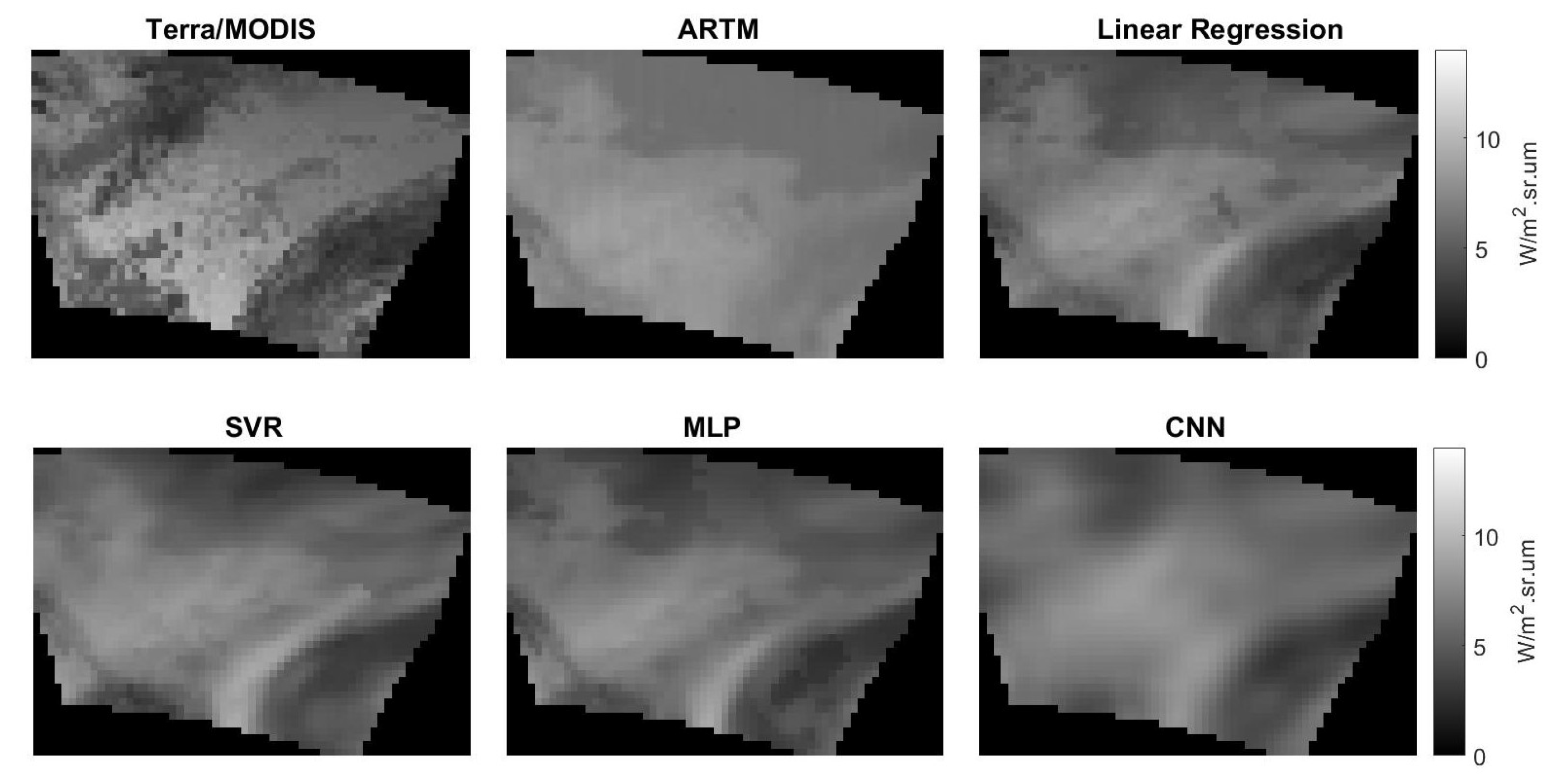
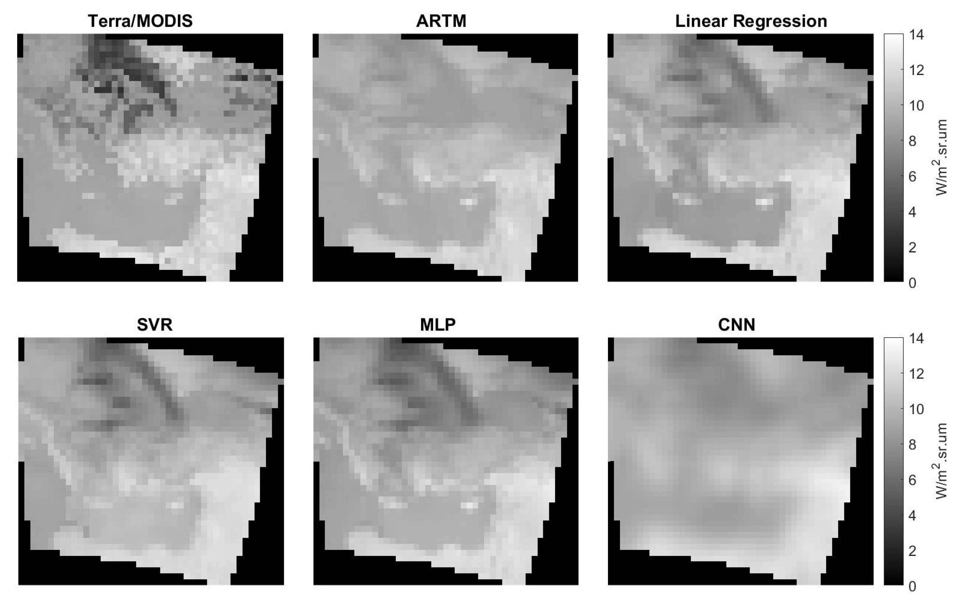
To visualize the results, Figure 8 displays predicted TOA thermal infrared data for one of the test images for the various models, with the Terra/MODIS down-sampled reference image displayed top left. Clouds (dark pixels) are clearly visible in the Terra/MODIS image, and slightly visible in the linear regression, SVR, and MLP models. However, the CNN produces estimated radiances that are more averaged over the scene, which can be explained by the use of spatial information around the pixel of interest to train the model. The ARTM model does not account for clouds well.

While built-in cloud models are available in MODTRAN to assist in predicting TOA radiance when clouds are present, they require knowledge of cloud type, cloud thickness, and base height. As mentioned earlier, MERRA-2’s cloud fraction variable does not agree with MODIS, and the other variables are not available in MERRA-2. Another test scene can be seen in Figure 9. As with the first scene, the ARTM did not account for clouds well and the CNN produced a smoother (averaged) predicted TOA thermal radiance image.

Table 1. RMSE, Standard deviation (STD) and Mean error [Mean] in W/m${}^2$·sr·$\mathsf{\mu }$m for land, water, and cloud cover.

Model	Total	Land	Water	Cloud
	RMSE (STD) [Mean]	RMSE (STD) [Mean]	RMSE (STD) [Mean]	RMSE (STD) [Mean]
ARTM	1.47 (1.43) [−0.36]	1.08 (1.06) [0.21]	0.62 (0.58) [−0.20]	2.35 (1.69) [−1.64]
Linear Regression	1.38 (1.33) [0.38]	1.32 (1.09) [0.75]	0.96 (0.85) [0.43]	1.72 (1.66) [−0.43]
SVR	1.43 (1.43) [−0.05]	1.27 (1.24) [0.31]	0.88 (0.87) [−0.11]	1.95 (1.80) [−0.75]
MLP	1.36 (1.33) [0.25]	1.28 (1.14) [0.59]	0.97 (0.93) [0.28]	1.70 (1.62) [−0.50]
CNN	1.41 (1.40) [0.17]	1.33 (1.13) [0.70]	0.82 (0.82) [0.06]	1.84 (1.63) [−0.84]

displays the RMSE, standard deviation, and mean error associated with the five different models for all scenes when compared to MODIS image data. Column two reports the total combined errors for all scenes. Columns three to five display the errors for land, water, and cloud cover classifications. The MODIS Land Cover maps [22] and Cloud Mask were used to classify land, water and cloud cover. For example, to calculate the errors where clouds were present, only test instances were evaluated where the MODIS Cloud Mask indicated cloudy. To calculate errors over land and water, only test instances where the MODIS Cloud Mask indicated probably clear and confident clear were evaluated. Mean errors were calculated by taking the average over the whole image and/or over each land cover type, after subtracting the predictions from Terra/MODIS band 31 radiance values.

Examining the mean values in Table 1, all models over-estimated cloud radiance compared to the Terra/MODIS reference values. This indicates that the models predict a higher radiance for those pixels instead of a low cloud radiance. The MLP has the lowest RMSE errors where clouds are present in a scene. For cloudless scenes, the ARTM model produced the lowest errors.

The percent prediction error was also used to measure error. This was calculated as the absolute value of the difference between Terra/MODIS radiance and model predicted divided by Terra/MODIS radiance:

$$\mathrm{error}=\frac{\left|\mathrm{Terra}/\mathrm{MODIS}-\mathrm{Model}\mathrm{Predicted}\right|}{\mathrm{Terra}/\mathrm{MODIS}}[\%].$$

(6)

The percent prediction error was calculated for several radiance levels as can be seen in

Table 2. Error percentage per radiance band.

Radiance	1.5 to <2	2 to <4	4 to <6	6 to <8	8 to <10	10 to <12	12 to <14
Range	W/m${}^2$·sr·$\mathsf{\mu }$m	W/m${}^2$·sr·$\mathsf{\mu }$m	W/m${}^2$·sr·$\mathsf{\mu }$m	W/m${}^2$·sr·$\mathsf{\mu }$m	W/m${}^2$·sr·$\mathsf{\mu }$m	W/m${}^2$·sr·$\mathsf{\mu }$m	W/m${}^2$·sr·$\mathsf{\mu }$m
Blackbody	211 to<221	221 to<250	250 to<271	271 to<288	288 to<303	303 to<316	316 to<328
Temperature	(K)	(K)	(K)	(K)	(K)	(K)	(K)
# of pixels	16	158	458	831	1546	514	16
ARTM	411%	107%	33%	11%	5%	9%	12%
Linear Regression	274%	71%	28%	10%	11%	10%	9%
SVR	293%	79%	31%	12%	10%	6%	11%
MLP	274%	68%	23%	10%	11%	8%	9%
CNN	293%	75%	25%	9%	10%	11%	12%

. The blackbody temperature ranges corresponding to the radiance levels at wavelength 10.97 microns (Terra/MODIS band 31 center wavelength) are displayed in the table below the radiance range for reference. The number of pixels used in each range to calculate the percent error are also displayed. From the table it can be seen that very large errors occur when the radiance values are below 6 W/m${}^2$·sr·$\mathsf{\mu }$m (below 271 K). This is consistent with the results in Table 1 where clouds (which are cold and therefore have low radiance values) have the highest RMSEs. Prediction errors were radiances were above 6 W/m${}^2$·sr·$\mathsf{\mu }$m varied between $5\%$ and $12\%$.

Error Analysis

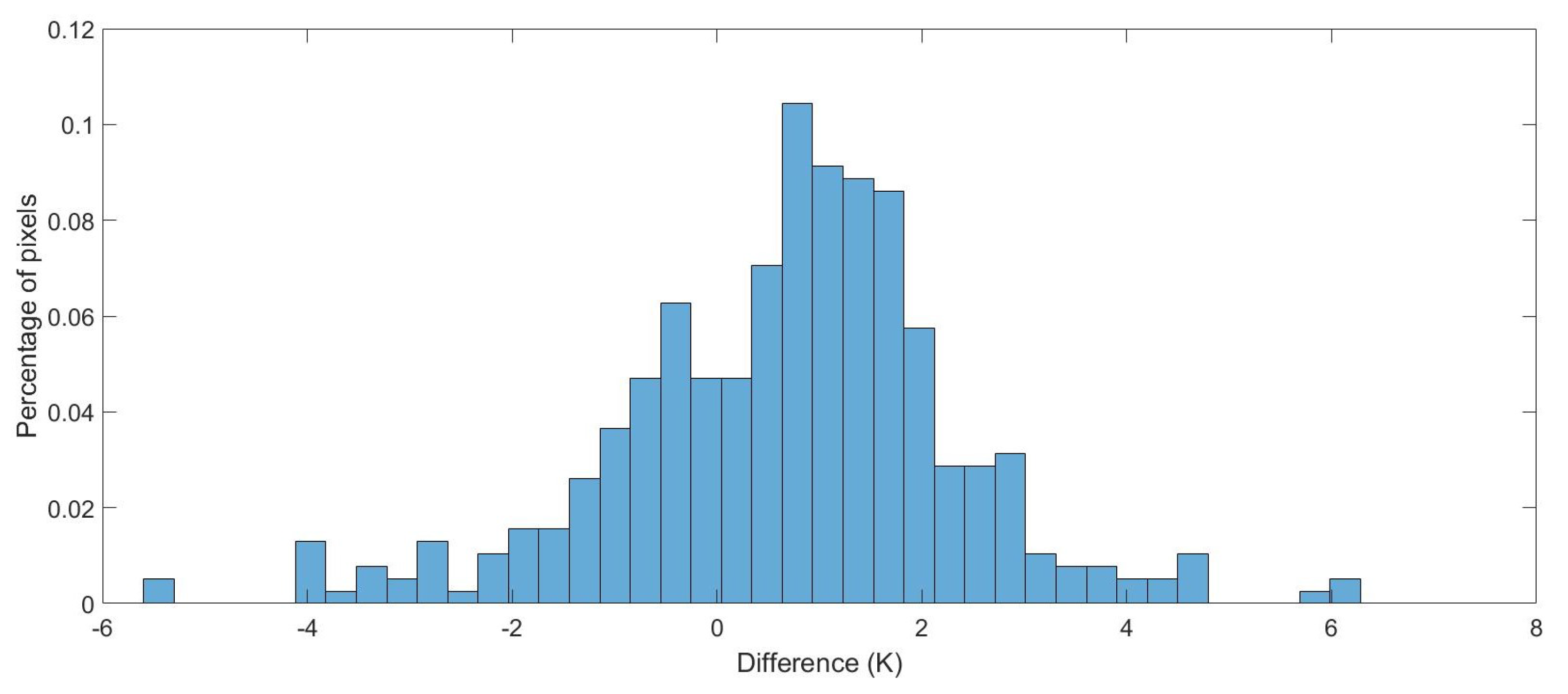
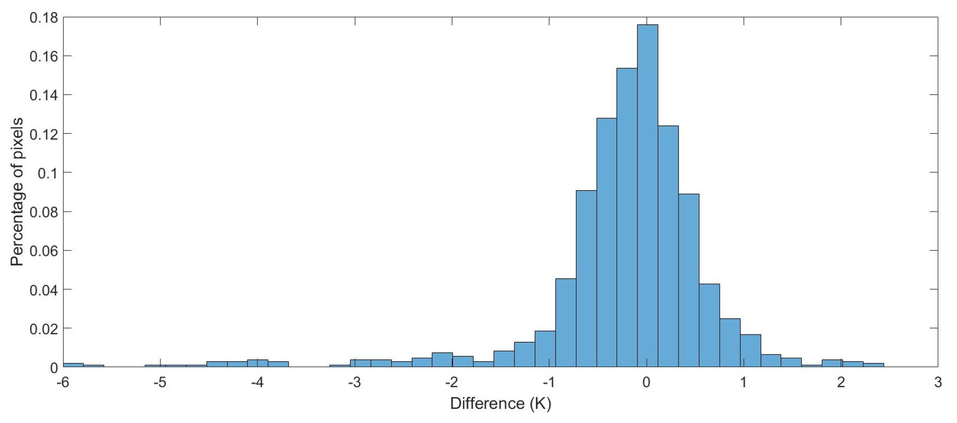
The relatively high RMSE values observed in Table 1, can partly be explained by (1) the MERRA-2 skin temperature used as input data and (2) the large difference in spatial resolution between the reference data (Terra/MODIS) and MERRA-2. The quality of the MERRA-2 skin temperature over land was assessed using the MODIS Land Surface Temperature product (MOD 11) where the MODIS Land Surface Temperature (LST) QC flag was set to pixel produced, good quality. This flag represents the highest quality data with respect to the LST product. A histogram of the difference between the MERRA-2 instantaneous skin temperature and the down-sampled MODIS LST can be seen in Figure 10. Differences ranged from $-5.6$ K to $6.3$ K with an RMSE of 1.82 K, a standard deviation of 1.70 K and a mean error of 0.68 K. Note that 1.82 K is approximately 0.18 W/m${}^2$·sr·$\mathsf{\mu }$m in Terra/MODIS band 31, thus 0.18 W/m${}^2$·sr·$\mathsf{\mu }$m of 1.08 W/m${}^2$·sr·$\mathsf{\mu }$m, or 17% of the error over land for the ARTM model displayed in Table 1, can be attributed to the MERRA-2 skin temperature variable.

MERRA-2 skin temperature over water was also evaluated. MODIS Sea Surface Temperature (MOD 28) was used as validation [34] (only pixels where the MODIS Quality Control (QC) flag was 0 (good) as recommended by the MODIS Sea Surface Temperature (SST) guide document [35]). Figure 11 displays the histogram of the differences between MODIS SST and MERRA-2 skin temperature. An RMSE of 1.05 K, standard deviation of 1.02 K, and a mean error of −0.25 K was found by evaluating 1080 grid points. As 1.05 K is approximately 0.1 W/m${}^2$·sr·$\mathsf{\mu }$m in Terra/MODIS band 31, approximately 0.1 W/m${}^2$·sr·$\mathsf{\mu }$m of the 0.62 W/m${}^2$·sr·$\mathsf{\mu }$m, or 16% of the error over water in the ARTM model displayed in Table 1, can be attributed to the use of the MERRA-2 skin temperature.

While the MERRA-2 skin temperature represents a large source of error, another possible source of error in the model prediction is due to the large difference in spatial resolution between the training data (MERRA-2) and the reference data (Terra/MODIS). Various interpolation techniques yielded different results. A comparison between a down-sampled Terra/MODIS scene using nearest neighbor and bilinear interpolation, resulted in respective differences in radiance values with an RMSE of 0.18 W/m${}^2$·sr·$\mathsf{\mu }$m. Down-sampling Terra/MODIS from 1 km spatial resolution to 0.5 × 0.625 degrees (approximately 50 km × 70 km at the equator) is a rather large resampling, such that high spatial frequencies in the MODIS scene will be averaged out in the down-sampled scene. Bilinear interpolation was used throughout this work to mitigate this effect.

5. Discussion and Summary

The goal of this research was to predict sensor reaching thermal radiance using the data from MERRA-2 with machine learning. This study also investigated the limitations and major sources of error in using atmospheric reanalysis data in predicting TOA thermal radiance. To estimate TOA radiance, five models were developed using both physics-based and machine learning approaches. MERRA-2 variables were used as input to the models. The physics-based model used the atmospheric radiative transfer model MODTRAN to predict TOA radiance. Two of the machine learning models were based on deep learning. Since Terra/MODIS band 31 was used as reference, all models were built to predict sensor reaching thermal radiance with center wavelength 10.97 $\mathsf{\mu }$m (corresponding to Terra/MODIS band 31 band center).

The MLP model produced the lowest overall error rates, with an RMSE of 1.36 W/m${}^2$·sr·$\mathsf{\mu }$m when compared to actual MODIS band 31 image data. This was mainly driven by the high RMSE of the ARTM model when clouds were present in the scene. Where no cloud was present, errors were significantly lower. The ARTM model predicted TOA radiance of cloudless scenes over land and water to within 1.08 W/m${}^2$·sr·$\mathsf{\mu }$m and 0.62 W/m${}^2$·sr·$\mathsf{\mu }$m, respectively. All machine learning models predicted TOA thermal radiance where clouds were present better than the physics based ARTM model. The percent error metric indicated that prediction errors of 12% and lower can be expected when the TOA radiance is above 6 W/m${}^2$·sr·$\mathsf{\mu }$m (approx. 271 K). When TOA radiance is below 6 W/m${}^2$·sr·$\mathsf{\mu }$m, which typically indicates the presence of clouds, errors are high for all models. When no prior knowledge of cloud cover is available, the MLP model is suggested for use, along with the error percentage table to indicate the confidence at various radiance values. If run time is not an obstacle, and knowledge of cloud cover is available, the use of MODTRAN is recommended.

This research investigated several sources of error. The first was the MERRA-2 skin temperature variable. MERRA-2 skin temperatures were assessed using the MODIS LST and SST products, since skin temperature plays a significant role in TOA thermal radiance. Taking the difference between MERRA-2 skin temperature and MODIS LST into account, when looking at the ARTM model, 17% of the RMSE over land can be explained. All models under predicted cloudless scenes over land, which could be explained by the MODIS LST that is on average 0.68 K higher than the MERRA-2 skin temperature. The differences in water temperature between MODIS SST and MERRA-2 skin temperature could further explain 16% of the error over water in the ARTM model. Another source of error resulted from the large difference in spatial resolution between the Terra/MODIS reference data (1 km × 1 km) and the reanalysis data (approximately 50 km × 70 km at the equator). Two different resampling methods were applied to one Terra/MODIS test scene. A comparison between the down-sampled MODIS test image using nearest neighbor and bilinear interpolation respectively resulted in an RMSE of 0.18 W/m${}^2$·sr·$\mathsf{\mu }$m.

The test dataset used was too small to analyze error as a function of season or region (e.g., this would require a large number of test scenes per region, season, etc.). In preliminary experiments, seasonality and spatial location were encoded as input to the model, but neither had an impact on performance and was not included in final models.

The supervised learning models used 27 layers of the air temperature and relative humidity profile data. This corresponds to about 21 km above sea level, which is in the lower stratosphere. Models with fewer layers (just troposphere) did not perform as well on the test data, which indicate that the atmospheric profiles into the lower stratosphere affect TOA thermal radiance. When all 42 levels were used as input to the supervised models, the test results were slightly worse than using only 27 levels. This may be due to the models overfitting on data that is not useful for making the inference, resulting in impaired generalization. The CNN model did not perform better than the MLP model. This may be due to the low spatial resolution of MERRA-2. Because the CNN input data spanned $9\times 9$ grid points (approximately 450 km × 650 km at the equator), it could have included unnecessary spatial information. It is challenging to interpret the features that neural networks are using to make their inferences, making their errors difficult to study. Development of visualization techniques for determining the spatial locations that a CNN used to make its inference are being heavily studied [36], and it would be interesting to see if these methods could be adapted to MLP models, enabling us to determine which input features had the biggest influence.

Since Terra/MODIS band 31 was used as reference, models were built to predict TOA thermal radiance with center wavelength of 10.97 $\mathsf{\mu }$m. If reference data is available at different thermal wavelengths, models can easily be extended to predict for these wavelengths.

Due to the disagreement in MERRA-2’s cloud fraction variable and the cloud mask in MODIS, we did not use any cloud information as direct input to the algorithms. However, all of the models have the relative humidity and air temperature profiles as input, which they could learn to use for inferring the possible presence of clouds. It would be interesting to further investigate why there are differences between clouds in MERRA-2 and MODIS, but this is beyond the scope of this study.

Future work includes the development of a model to predict clouds from the MERRA-2 profile data to improve the models described in this work. The ARTM model could be changed to incorporate built-in MODTRAN cloud settings for grid points where clouds are present. The machine learning models could either be trained separately for cloud and no cloud points or ensembling could be used, which is where several models are trained and then averaged to produced better results.