Integration of Absorption Feature Information from Visible to Longwave Infrared Spectral Ranges for Mineral Mapping

Abstract

Merging hyperspectral data from optical and thermal ranges allows a wider variety of minerals to be mapped and thus allows lithology to be mapped in a more complex way. In contrast, in most of the studies that have taken advantage of the data from the visible (VIS), near-infrared (NIR), shortwave infrared (SWIR) and longwave infrared (LWIR) spectral ranges, these different spectral ranges were analysed and interpreted separately. This limits the complexity of the final interpretation. In this study a presentation is made of how multiple absorption features, which are directly linked to the mineral composition and are present throughout the VIS, NIR, SWIR and LWIR ranges, can be automatically derived and, moreover, how these new datasets can be successfully used for mineral/lithology mapping. The biggest advantage of this approach is that it overcomes the issue of prior definition of endmembers, which is a requested routine employed in all widely used spectral mapping techniques. In this study, two different airborne image datasets were analysed, HyMap (VIS/NIR/SWIR image data) and Airborne Hyperspectral Scanner (AHS, LWIR image data). Both datasets were acquired over the Sokolov lignite open-cast mines in the Czech Republic. It is further demonstrated that even in this case, when the absorption feature information derived from multispectral LWIR data is integrated with the absorption feature information derived from hyperspectral VIS/NIR/SWIR data, an important improvement in terms of more complex mineral mapping is achieved.

1. Introduction

Modern remote sensing has become a novel tool, not only for detecting and quantifying geological materials [1], but also for monitoring dynamic processes and induced changes in their physical/chemical properties [2,3,4,5,6]. Multispectral and superspectral imagery have been effectively used for mapping geology/minerals [7,8,9,10,11] as well as for monitoring mining impacts [12,13,14,15,16,17,18,19]. However, with a low number of rather broad spectral bands, these systems provide only discrete spectral information (e.g., the state-of-the-art Sentinel-2 sensor has 13 spectral bands [20]. On the other hand, data with very high spectral resolution (hundreds of narrow bands)—known in the remote sensing community as hyperspectral (HS) or imaging spectroscopy (IS) data—are nowadays capable of providing a continuous spectrum throughout the whole spectral range (0.4–13 µm). These systems are mainly available for aerial data acquisition; however, new hyperspectral satellite systems will be lunched in the near future [21,22,23,24,25].

The IS data can cover different spectral ranges from visible (VIS, 0.4–0.7 µm) through the near infrared (NIR, 0.7–1.0 µm) and shortwave infrared (SWIR, 1.0–2.5 µm) to even longer wavelengths of the thermal region (longwave infrared: LWIR, 8–13 µm). Within the VIS/NIR/SWIR/LWIR regions specific or combined absorptions (called absorption features from now on) can be found, caused by the electronic transition of Fe-bearing minerals (VIS/NIR region) and by the molecular vibration of specific chemical groups (e.g., OH⁻, CO₃, Si–O) (SWIR and LWIR spectral regions). Considering the main mineralogical groups, the VIS/NIR parts of the electromagnetic (EMS) spectrum allow for mapping surfaces with a high concentration of Fe³⁺-bearing minerals (e.g., hematite, goethite and jarosite) [6,26,27,28] and SWIR is useful in detecting carbonates, clay minerals and salts [29,30,31]. On the other hand, the VNIR and SWIR portions of the EMS are not optimal for detecting the main constituents of igneous rocks, quartz and feldspars due to their lack of absorption features in the optical part of the EMS. These minerals can be mapped using the thermal LWIR region [32,33,34,35,36].

Clearly, optical and thermal IS data, when used together, allow different varieties of minerals to be mapped and thus allow lithology mapping in a more complex way. The synergy effect of merging both ranges (optical and thermal) was demonstrated in examples of soil proximal sensing [37,38,39]. Considering mineral mapping, as stated by McDowell and Kruse [40], the majority of the previous work exploiting spectral IS data has focused on data from a single wavelength range, typically the VNIR, SWIR or LWIR. Few studies have taken advantage of data from the full VIS/NIR, SWIR, and LWIR spectral range, whereas the different spectral ranges were analysed and interpreted separately [41,42,43] and the full-range information was not actually combined into a single integrated data product. This limits the complexity of the final interpretation as spectral and spatial associations or patterns may be too complex to be seen by the naked eye and thus may remain hidden.

Recently, Kruse [41] proposed integrating the individual mapping results derived from AVIRIS (VIS/NIR/SWIR) and HyTES data (LWIR) and combining them using geologically directed logical operators. In the following study by McDowell and Kruse [40], spectral information from the individual VIS, NIR, SWIR and LWIR ranges was first analysed independently and then the resulting compositional information, in the form of image endmembers and apparent abundances, was integrated using ISODATA cluster analysis. They demonstrated that the integrated map provided additional compositional information that was not evident in the VIS, NIR, SWIR, or LWIR data alone, and concluded that their analysis allowed for more complete and accurate compositional mapping.

This study tested whether the multiple absorption features, which are directly linked to the mineral composition and are present though the VIS/NIR/SWIR and LWIR ranges, can be:

• automatically derived throughout the different spectral ranges
• integrated and, moreover, if this new dataset can be successfully used for final mineral/lithology mapping

To map multiple absorption feature parameters automatically, a toolbox was used that was developed using Interactive Data Language (IDL). The biggest advantage of such an approach is that it allows the issue of prior definition of the endmembers to be overcome; this is a requested routine used for all widely-used spectral mapping techniques (e.g., Spectral angle mapping SAM [44], Spectral feature fitting SFF e.g., [45,46] and Spectral unmixing [47,48]. Two different airborne image datasets were analysed, HyMap (HyVista Corp., Australian airborne imaging spectrometer, VIS/NIR/SWIR image data) and Airborne Hyperspectral Scanner (AHS, LWIR image data), both datasets were acquired over the Sokolov open-cast lignite mines in the Czech Republic. It is further demonstrated that even in this case, when the absorption feature information derived from multispectral LWIR data is integrated with the absorption feature information derived from hyperspectral VIS/NIR/SWIR data, it is an important contribution and improvement in terms of more complex mineral mapping.

2. Materials and Methods

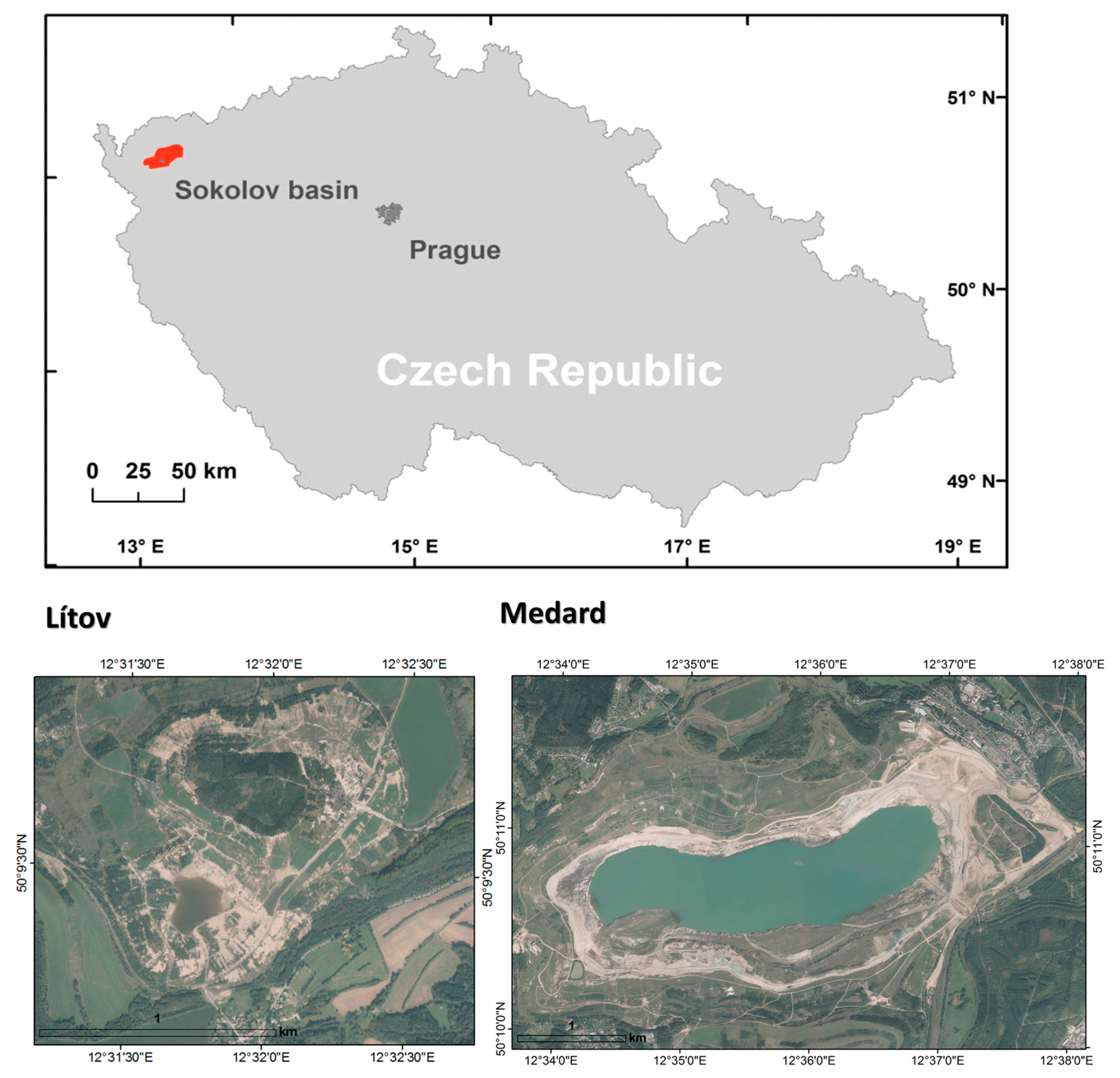
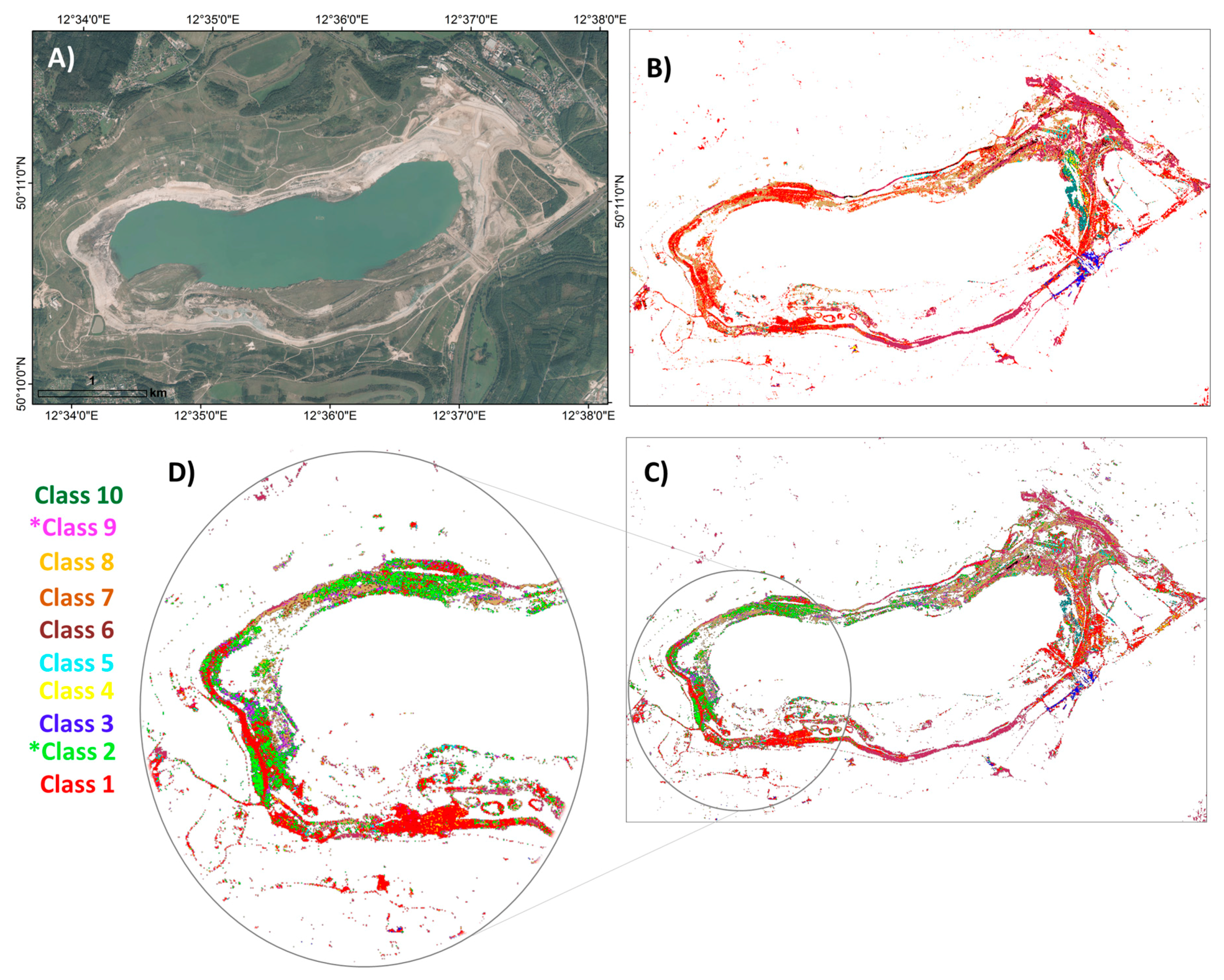
2.1. Test Site

The study was performed in the Sokolov basin in the western part of the Czech Republic (Figure 1), in a region affected by long-term extensive lignite mining. The basement of the Sokolov Basin is formed of pre-Variscan and Variscan metamorphic complexes (recorded metamorphism from Devonian to Lower Carboniferous periods) of the Eger, Erzgebirge, Slavkov Forest, Thuring-Vogtland Crystalline Units and granitoids of the Karlovy Vary Pluton. The upper portions of these rocks are frequently weathered to kaolinitic residue. The basal late Eocene Staré Sedlo Formation is formed of well-sorted fluvial sandstones and conglomerates and is overlain by a volcano–sedimentary complex up to 350 m thick, which contains three lignite seams with variable sulphur (S) content. Long-term open cast mining required the removal of up to 180 m of thick overburden (Cypris clays), which was stockpiled and replaced after the lignite was extracted. At the dumps, the material consists mostly of weathered volcanic tuffs and Cypris clays, which can be characterised as well-laminated clays with a dominant kaolinite content; however, different varieties of mineralogical composition are common (e.g., the presence of montmorillonite, illite with admixtures of Ca–Mg–Fe carbonates, sulphates, sulphides, analcite, Mg–micas and bitumen [49]. Due to the presence of S in the coal, both active and abandoned lignite mines are affected by acid mine drainage (AMD) [50,51].

Considering the Sokolov site, under various research projects (HypSo, EO-MINERS, DeMinTIR), numerous studies have been published demonstrating how hyperspectral imaging data can be utilised to quantitatively model the substrate pH [6,52], map mineral composition [41], estimate mine water pollution [53] and assess tree health [54,55,56]. This study focused on the Lítov dump and the abandoned open pit called Medard (Figure 1), as no human activities were conducted between 2010 and 2011 at these two sites, the years when the two aerial image datasets, HyMap and AHS, were acquired, thus these two sites faced no changes regarding the relief and material transport between 2010 and 2011.

2.2. Data

2.2.1. Airborne Imaging Datasets and Their Pre-Processing

Two different airborne image datasets acquired over the Sokolov basin were used in this study. The HyMap image data was acquired in 2010 (August 27) during the HyEUROPE 2010 flight campaign using the HyMap (HyVista Corp., HyVista Corporation Pty Ltd., Baulkham Hills, NSW, Australia) airborne imaging spectrometer. The HyMap sensor records image data in 126 narrow spectral bands covering the entire spectral interval between 0.450 and 2.480 µm of the spectral range with a Full Width Half Maximum (FWHM) of 15 nm and a ground field of view of 4 m. The resulting ground pixel resolution of the image datasets was 5 m. In order to successfully pre-process the hyperspectral data, supportive calibration and validation ground campaigns were organised simultaneously with the HyMap data acquisition. At the selected homogenous targets the ground measurements were acquired by an ASD FieldSpec-3 spectroradiometer to properly calibrate as well as validate the image data and to enable: (i) atmospheric correction of the airborne hyperspectral images and (ii) retrieval of surface reflectance values for further verification. The final atmospheric correction was performed in the ATCOR-4 software package [57] using the MODTRAN 4 physical model of the atmosphere [58]. A detailed description of the HyMap data preprocessing can be found in Adar et al. [59].

The second image dataset was acquired by the Airborne Hyperspectral Scanner (AHS) in collaboration with the Spanish Aerospace Institute (INTA) as a set of day (19 July 2011) and night image data (22 July 2011). The AHS is an imaging 80-band line-scanner radiometer with 63 bands in the visible-near infrared (VNIR) and shortwave infrared (SWIR) regions, seven bands in the mid-wave infrared (MWIR) region and 10 bands in the longwave infrared (LWIR) region [60]. However, due to cloud cover in the daytime image, it was only possible to use the cloud-free night-time LWIR data. These were acquired after a dry day, on a clear night with no precipitation. The flight lines were acquired at an altitude of 2 km above ground level, resulting in a 5-m pixel size (the same pixel size as the HyMap dataset). The temperature and emissivity were derived from the sensor radiance using the approach described in detail by Notesco et al. [42].

Both datasets were geo-corrected using on-board navigation information. After that both datasets were further georeferenced to the very high spatial resolution aerial orthophotos (pixel size = 0.5 m) achieving sub-pixel positional accuracy. To avoid any spatial misalignments, both datasets were resampled to a 10-m spatial resolution using nearest-neighbour resampling.

2.2.2. Ground Verification Data

Various soil/substrate samples were collected in the field in both years (2010 and 2011) and analysed with a Philips X’Pert X-ray Diffractometer (XRD) at the Czech Geological Survey to resolve their mineralogy. The X-ray powder diffraction patterns were obtained using monochromatic (CuKα) radiation and a graphite secondary monochromator. The whole-sample random patterns were collected in the angular range from 2° to 70° (2ϴ) with steps of 0.05° (2ϴ). Oriented clay-fraction specimens (fraction < 2 μm) were prepared by a conventional sedimentation method [61]. The oriented clay specimens were analysed after air-drying and after saturation for 10 h with ethylene–glycol vapour at 60 °C. Their diffraction data were acquired in the angular range of 2–50° (2ϴ) with steps of 0.05° (2ϴ). Mixed-layered minerals were identified by comparing the analysed XRD patterns of the ethylene-glycolated oriented clay fraction with the modelled XRD patterns obtained by NEWMOD code [61].

2.3. Methods

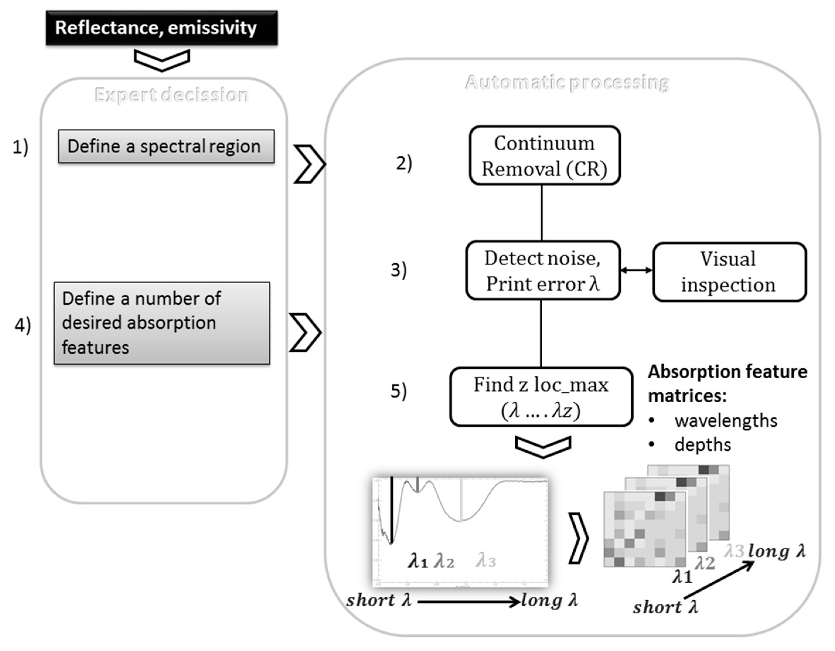
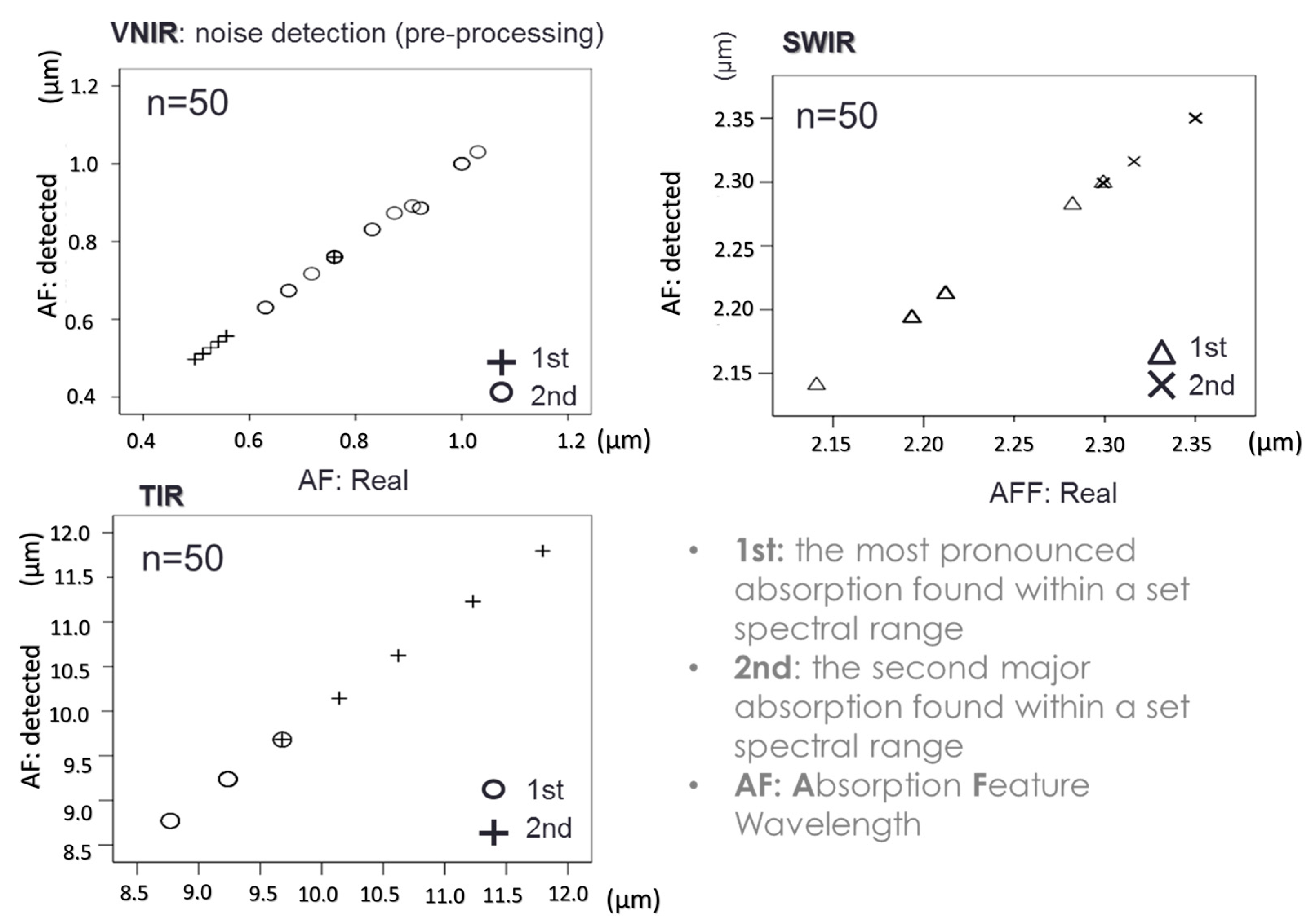
2.3.1. Absorption Wavelength Mapping

To map absorption features, namely absorption wavelengths and depths, new tools, which are described here for the very first time, were programmed to allow automatic detection of multiple absorption feature parameters. The tools—e.g., called QUANTools—have been created using IDL programming language (ENVI/IDL: version 5.0 and higher, [62]).

The tools can process both spectral libraries and hyperspectral image data. They consist of basic modules (GUIs) (Figure 2) allowing users to:

• Define a spectral range within the visible (VIS), near-infrared (NIR), shortwave infrared (SWIR) or thermal (TIR) spectral regions. Different spectral ranges can be defined and analysed consequently, one after another.
• Employ Continuum Removal (CR)—A standard method to normalise the spectrum, to a departure from the norm [63].
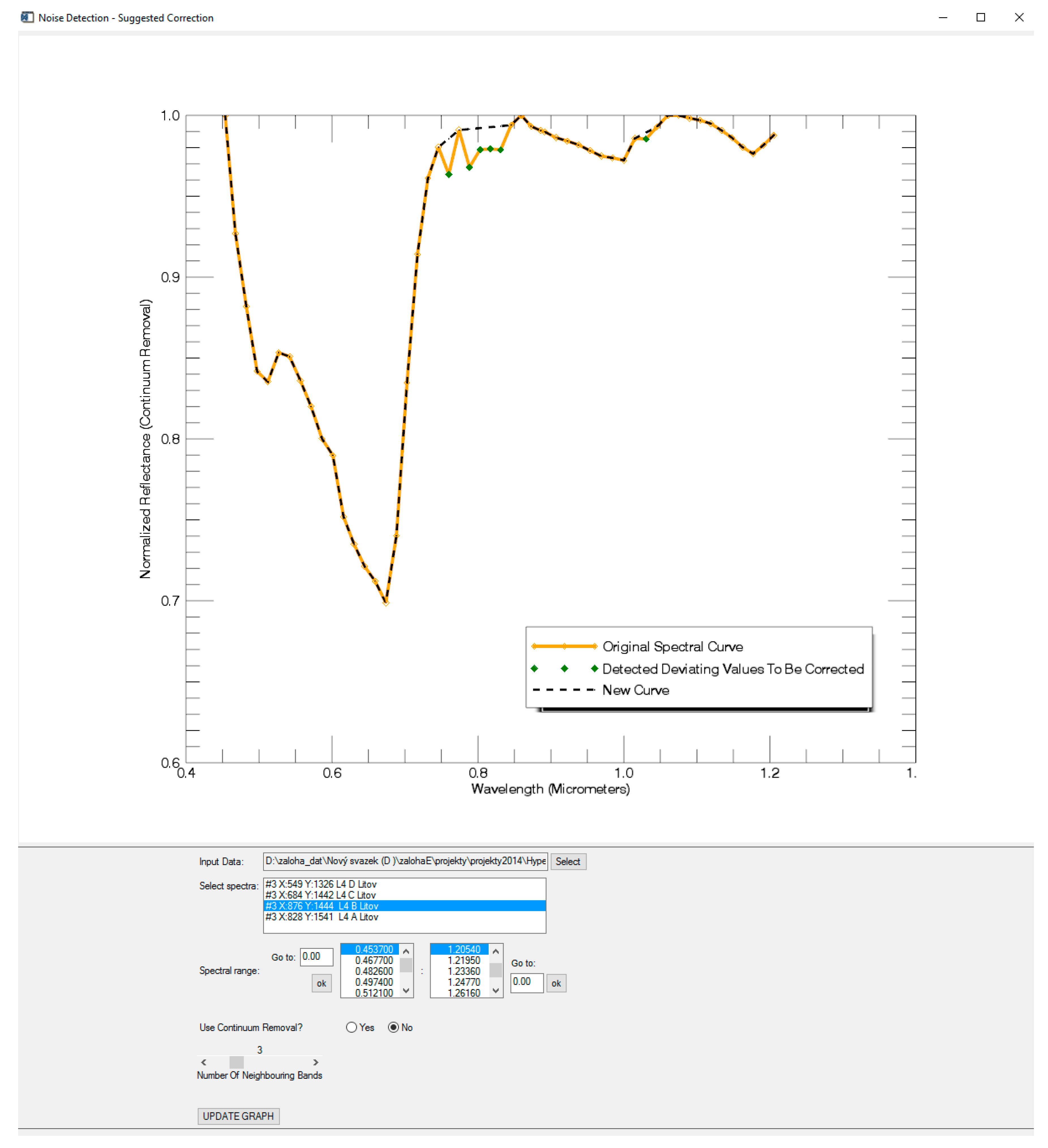
• Detect bad spectral bands—A user can use a graphical interface to detect and correct bad (noisy) spectral bands.
• Define a number of desired absorption features to be detected within a set spectral range: the user can decide whether to detect an absolute absorption (the most pronounced one) or to define a number of multiple absorption features that can be identified within a set spectral range.
• Calculate absorption feature parameters (absorption wavelengths and depths): after correcting noisy bands, the trend of a spectral curve is analysed and saddle points—the local absorption maximum wavelengths (loc_max)—are detected and assigned to an image matrix. The detected absorptions are sorted in ascending order from shorter to longer wavelengths. Additionally, a corresponding absorption depth matrix is also calculated for each absorption feature.

The only decisions made by an operator/expert are to define the spectral region (Figure 2, step 1) and the number of desired absorption features mapped in each spectral region (Figure 2, step 4). All the other steps are done automatically when processing the datasets. A detailed explanation of the processing steps available in the toolbox is given in Section 2.3.2, below.

2.3.2. The Toolbox (QuanTools) Description

QuanTools can be used for spectral absorption band mapping using spectral libraries or hyperspectral image data (Figure 2). A user first defines the spectral range to be analysed within the visible (VIS), near-infrared (NIR), shortwave infrared (SWIR) or longwave infrared (LWIR) regions (Figure 2, step 1). Different spectral ranges can be defined and analysed after one another. Next comes continuum removal (CR, [63]), by which the continuum—that is, a convex hull of straight-line segments, is fitted over a reflectance spectrum and subsequently removed by division or rationing (Figure 2, step 2). The next step is noise detection and removal using local minima of the spectral curve defined as:

$$R=\left\{\begin{array}{c}1if{\rho }_{CR}\left(\lambda -1\right)\ge {\rho }_{CR}\left(\lambda \right)\\ 0if{\rho }_{CR}\left(\lambda -1\right)<{\rho }_{CR}\left(\lambda \right)\end{array}\right\}$$

(1)

$$if\left[R\left(\lambda -1\right)=1\right]\wedge \left[R\left(\lambda \right)=0\right]\Rightarrow localminimum,$$

(2)

where ${\rho }_{CR}\left(\lambda \right)$ and ${\rho }_{CR}\left(\lambda -1\right)$ are the values of the spectral curve after Continuum Removal and R is an auxiliary variable. When the local minima are found, it has to be decided whether the value represents noise or not. The decision is based on two sets of values (a defined number of surrounding bands, e.g., called a spectral window)—derived from bands placed before and after the local minimum:

$$A\left(\lambda \right)=\left\{\begin{array}{c}{\rho }_{CR}\left(\lambda -nn\right);\left(\lambda -nn\right)\\ ⋮\\ {\rho }_{CR}\left(\lambda -2\right);\left(\lambda -2\right)\\ {\rho }_{CR}\left(\lambda -1\right);\left(\lambda -1\right)\end{array}\right\}$$

(3)

$$\left(\lambda \right)=\left\{\begin{array}{c}{\rho }_{CR}\left(\lambda +1\right);\left(\lambda +1\right)\\ {\rho }_{CR}\left(\lambda +2\right);\left(\lambda +2\right)\\ ⋮\\ {\rho }_{CR}\left(\lambda +nn\right);\left(\lambda +nn\right)\end{array}\right\},$$

(4)

where $A\left(\lambda \right)$ represents the set of surrounding bands before the local minimum, $B\left(\lambda \right)$ represents the set after the local minimum, and nn is the number of surrounding bands. Then the minimum values of these sets are detected as:

$$A_{min}\left(\lambda \right)=\min {\rho }_{CR}\in A\left(\lambda \right)$$

(5)

$$B_{min}\left(\lambda \right)=\min {\rho }_{CR}\in B\left(\lambda \right).$$

(6)

The minimum of the spectral window ($A_{min}\left(\lambda \right)$, $B_{min}\left(\lambda \right)$) is compared to the local minimum ${\rho }_{CR}\left(\lambda \right)$. Using this comparison, the noise is detected as follows:

$$[B_{min}\left(\lambda \right)<{\rho }_{CR}\left(\lambda \right)]\wedge \left[A_{min}\left(\lambda \right)>{\rho }_{CR}\left(\lambda \right)\right]:$$

(7)

$$if{\rho }_{CR}\in A\left(\lambda \right)<{\rho }_{CRmax}\in B\left(\lambda \right)\Rightarrow print\left\{\begin{array}{c}Err\left(\lambda -1\right)\\ Err\left(\lambda -2\right)\\ ⋮\\ Err\left(\lambda -n\right)\end{array}\right\};n\le nn$$

$$if\left\{\begin{array}{c}\left(\lambda +1\right)\\ \left(\lambda +2\right)\\ ⋮\\ \left(\lambda +nn\right)\end{array}\right\}\in B\left(\lambda \right)<{\rho }_{CRmax}\left(\lambda \right)\in B\left(\lambda \right)\Rightarrow print\left\{\begin{array}{c}Err\left(\lambda +1\right)\\ Err\left(\lambda +2\right)\\ ⋮\\ Err\left(\lambda +n\right)\end{array}\right\};n\le nn$$

$$[A_{min}\left(\lambda \right)<{\rho }_{CR}\left(\lambda \right)]\wedge \left[B_{min}\left(\lambda \right)>{\rho }_{CR}\left(\lambda \right)\right]:$$

(8)

$$if{\rho }_{CR}\in B\left(\lambda \right)<{\rho }_{CRmax}\in A\left(\lambda \right)\Rightarrow print\left\{\begin{array}{c}Err\left(\lambda +1\right)\\ Err\left(\lambda +2\right)\\ ⋮\\ Err\left(\lambda +n\right)\end{array}\right\};n\le nn$$

$$if\left\{\begin{array}{c}\left(\lambda -1\right)\\ \left(\lambda -2\right)\\ ⋮\\ \left(\lambda -nn\right)\end{array}\right\}\in A\left(\lambda \right)<{\rho }_{CRmax}\left(\lambda \right)\in A\left(\lambda \right)\Rightarrow print\left\{\begin{array}{c}Err\left(\lambda -1\right)\\ Err\left(\lambda -2\right)\\ ⋮\\ Err\left(\lambda -n\right)\end{array}\right\};n\le nn,$$

where $Err\left(\lambda \right)$ represents noise (“bad” bands).

These error values are recalculated using the values of the surrounding bands (their number is defined by a spectral window size). For sample spectral data, a graphical interphase can be used to set up a spectral window size and check the corrected spectral curves (Figure 3, step 3). This allows the user to compare the results of different settings and finally employ a correction that is optimally tuned for the data under analysis.

After a noise-cleaned image is retained, the operator decides how many absorption features are to be derived (Figure 2, step 4) and the analysis is done automatically (Figure 2, step 5) using the following processing:

$$CRdepth\left(\lambda \right)=1-{\rho }_{CR}\left(\lambda \right).$$

(9)

Then the trend of the spectrum is analysed in a similar way to noise detection. First the saddle points (the local absorption maxima) are detected using these conditions:

$$R_{ij}=\left\{\begin{array}{c}1ifCRdepth{\left(\lambda \right)}_{ij}\ge CRdepth{\left(\lambda -1\right)}_{ij}\\ 0ifCRdepth{\left(\lambda \right)}_{ij}<CRdepth{\left(\lambda -1\right)}_{ij}\end{array}\right\}$$

(10)

$$if[R{\left(\lambda -1\right)}_{ij}=1\left]\wedge \right[R{\left(\lambda \right)}_{ij}=0]\Rightarrow printLoc\_ma{x}_{ij},$$

where R is an auxiliary variable that records increase (1) or decrease (0). During this step, local absorption maximum depths and wavelengths are registered:

$$Lo{c}_{max}{}_{ij}=\left\{\begin{array}{c}Lo{c}_{max}{}_{1}depth{\left(\lambda \right)}_{ij};Lo{c}_{max}{}_1{\left(\lambda \right)}_{ij}\\ Lo{c}_{max}{}_{2}depth{\left(\lambda \right)}_{ij};Lo{c}_{max}{}_2{\left(\lambda \right)}_{ij}\\ ⋮\\ Lo{c}_{max}{}_{nm}depth{\left(\lambda \right)}_{ij};Lo{c}_{max}{}_{nm}{\left(\lambda \right)}_{ij}\end{array}\right\}.$$

(11)

A set number of desired absorption features is detected as the most pronounced local absorption maxima (a set number of the most pronounced absorptions according to the absorption depths). If the desired number is larger than the number of local maxima detected, the final array is completed by zero values:

$$Lo{c}_{max}{}_{ij}=\left\{\begin{array}{c}Lo{c}_{max}{}_{1}depth{\left(\lambda \right)}_{ij};Lo{c}_{max}{}_1{\left(\lambda \right)}_{ij}\\ Lo{c}_{max}{}_{2}depth{\left(\lambda \right)}_{ij};Lo{c}_{max}{}_2{\left(\lambda \right)}_{ij}\\ ⋮\\ Lo{c}_{max}{}_{To{t}_{nm}}depth{\left(\lambda \right)}_{ij};Lo{c}_{max}{}_{nm}{\left(\lambda \right)}_{ij}\\ 0;0\\ ⋮\\ 0_{nm};0_{nm}\end{array}\right\}.$$

(12)

Finally, the local absorption maximum features are assigned to image matrices. For z absorption features, two matrices with z bands are created; one has the absorption wavelengths assigned, while the second one has corresponding absorption depths assigned, respectively.

2.3.3. Specific Setting of the QUANTools

The main aim was to test if the major absorption features present though the VIS/NIR/SWIR and LWIR ranges can be (i) derived and integrated into one raster dataset; or (ii) successfully used for a final mineral mapping. The spectral ranges from which the absorption feature parameters were derived were defined as follows: VIS/NIR (HyMap): 0.450–1.200 µm, SWIR (HyMap): 2.100–2.400 µm and LWIR (AHS): 8.500–12.500 µm. Noise detection and correction was employed to the VIS/NIR reflectance (0.450–1.200 µm) and the spectral window was set to 3 (three spectral bands before and after the local minimum were analysed). The number of absorption features to be mapped in each spectral region was set to 2. As a result, two new raster datasets were derived for each spectral range, one having assigned the two major absorption wavelengths and the second raster dataset with corresponding absorption depths.

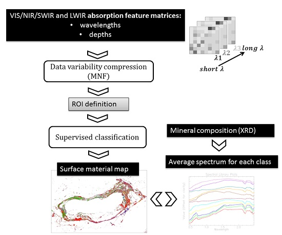
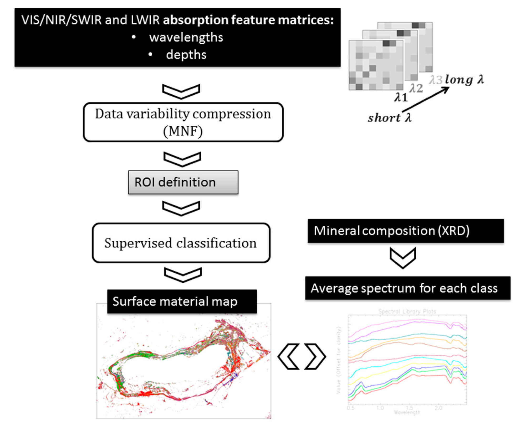
2.3.4. Integration of Absorption Feature Information Detected In VIS/NIR/SWIR and LWIR Data and Further Classification

After the wavelength mapping was employed to different spectral ranges, it was necessary to find a way to further integrate the absorption feature mapping results (Figure 4), more specifically the absorption wavelength and depth matrices. The MNF transformation [64] was employed to compress the data variability of these image matrices (six raster absorption wavelength matrices and six raster absorption depth matrices).

The intention was to test what the advantage will be of adding LWIR data (AHS) to the further mineral classification compared to using only the VIS/NIR/SWIR data (HyMap). Therefore, the MNF transformation was employed for two different scenarios:

• the MNF transformation was used so as to be comprised of only eight absorption wavelength/depth matrices derived on the basis of the HyMap data (VIS/NIR: two absorption wavelength and two absorption depth matrices, SWIR: two absorption wavelength and two absorption depth matrices)
• the MNF was employed to comprise of all 12 absorption wavelength/depth matrices derived from both HyMap and AHS datasets (in addition to eight absorption wavelength and depth matrices derived from the HyMap data, two absorption wavelength and two absorption depth matrices derived for the AHS data were added).

For each scenario, the first three MNF bands were visually analysed further to identify training areas (ROIs) representing different material/surfaces. The ROIs were defined as representative pixels of different colour clusters/regions. These were easy to identify when MNF1/MNF2/MNF3 images were displayed as RGB (Figure 5). The ROIs were then used for further supervised classification. In this case the simple non-parametric supervised (parallelepiped) classification was employed [65,66,67], which uses a simple decision rule to classify multispectral data. The parallelepiped classifier uses the threshold of each class signature to determine if a given pixel falls within the class or not. The thresholds specify the dimensions (in standard deviation units) of each side of a parallelepiped surrounding the mean of the class in the feature space. The best results (e.g., class separability, lowest number of unclassified pixels) were achieved when the upper and lower limits of each parallelepiped were set to ±1.5 standard deviations. In the last step, the classifications were overlaid over the original HyMap and AHS image data and the average spectrum from the original HyMap and AHS image data was computed for each class to (i) ensure that each class represents different surface material (is represented by a unique spectral signature) and (ii) be able to describe the mineral composition of each class when interpreting the spectral property.

3. Results

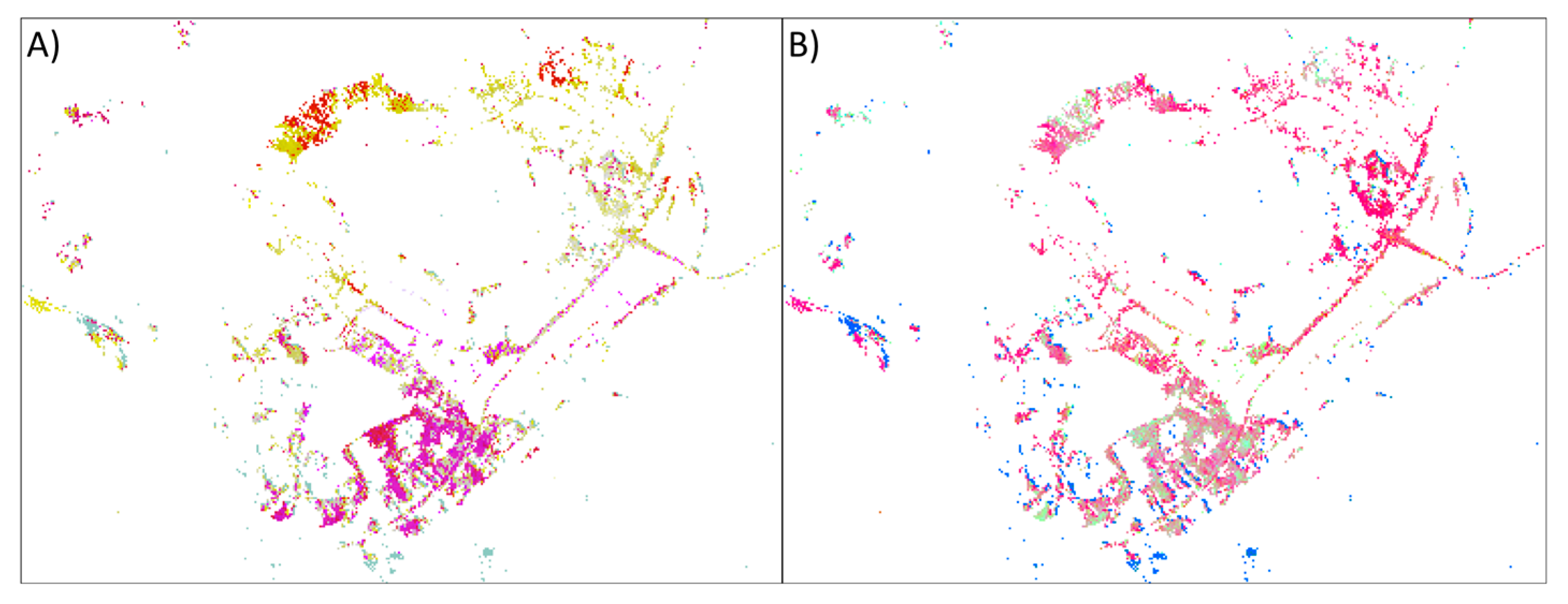
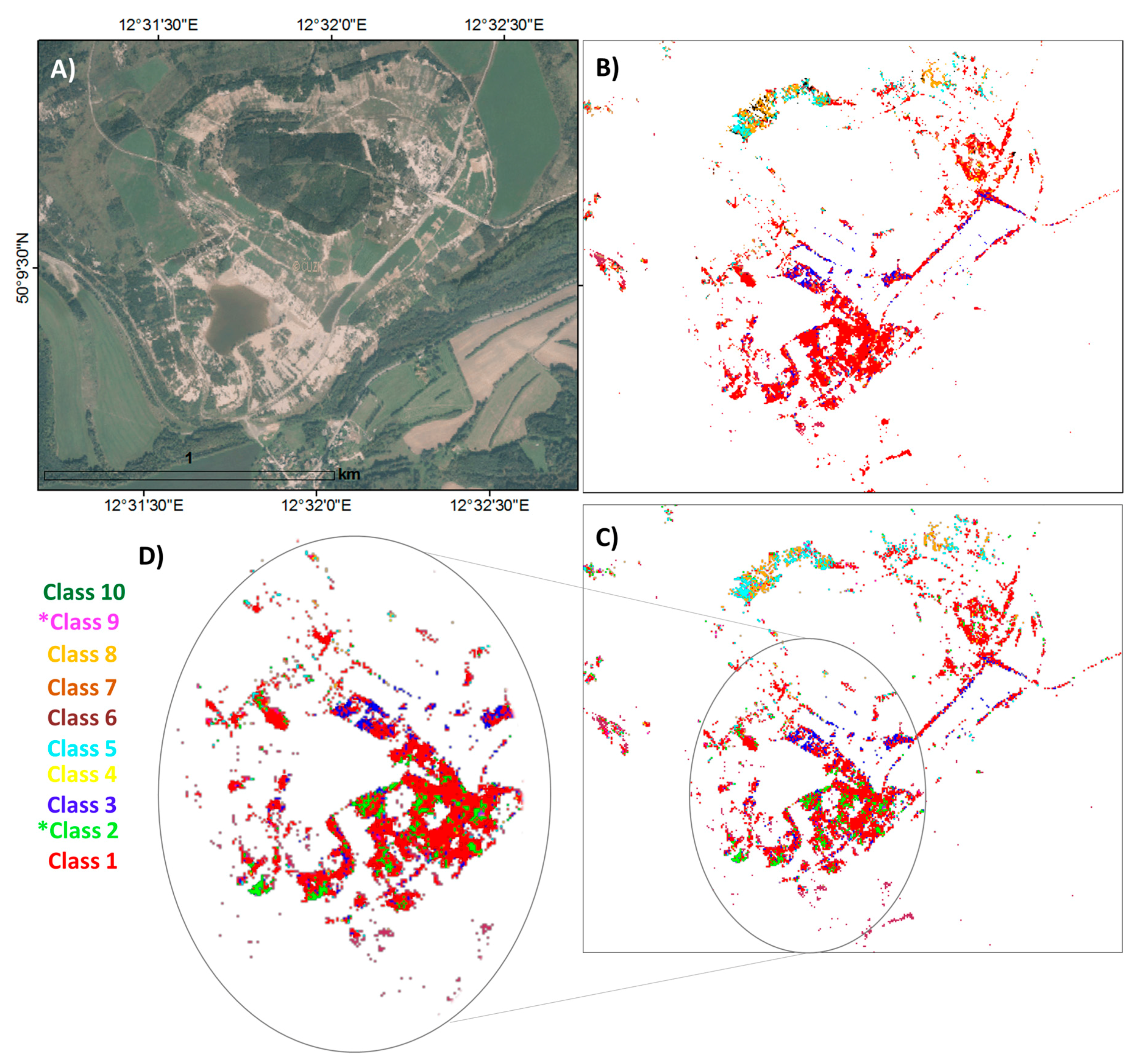
3.1. Full-Range (VNIR, SWIR and LWIR) Absorption Wavelength Mapping and Further Classification

The intention was to detect the two most pronounced absorptions within the VIS/NIR, SWIR (both HyMap dataset) and LWIR (AHS dataset) regions. To validate if the wavelengths were detected correctly, the absorption wavelength positions were manually derived from 50 different image pixels of the HyMap and AHS data representing different material/surfaces, and they were compared with the absorption wavelength positions of corresponding pixels detected by QaunTools (Figure 6). Only a small deviation in the NIR range (around 0.900 µm) was detected due to the smoothing employed for the VIS/NIR spectral region prior to wavelength mapping. The wavelength positions of all the other absorption features in the SWIR and LWIR regions were detected without any shifts or errors.

As described in the Methods an MNF transformation was employed to the absorption feature mapping results, first when using those derived from the HyMap data only (Scenario 1) and secondly to those derived from both the HyMap and the AHS data (Scenario 2). For each scenario, the ROIs were constructed using RGB colour compositions of the first three MNF bands and these ROIs were consequently used to employ a supervised parallelepiped classification. As a result, eight classes, which were the same for both classifications (Scenarios 1 and 2), were mapped (Figure 7B and Figure 8B). In the case of Scenario 2, where absorption feature parameters derived from both datasets (HyMap and AHS) were used for the consequent mineral mapping, it was possible to map the addition of two classes (Figure 7C and Figure 8C: *Class 2 and *Class 9). Figure 9 and Figure 10 show the average class spectrum derived from the HyMap data and the AHS data, respectively. The spectral property of these classes is further discussed and linked with the mineralogy in the following text.

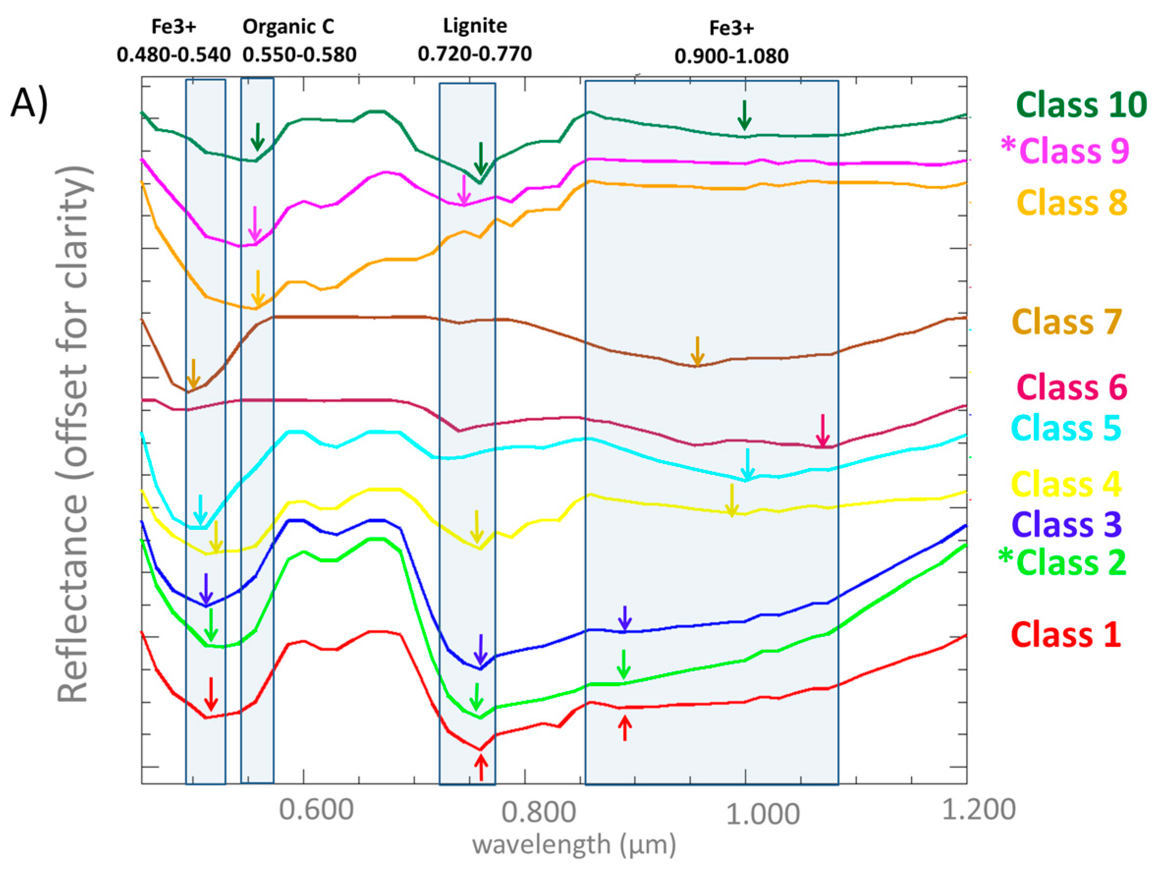
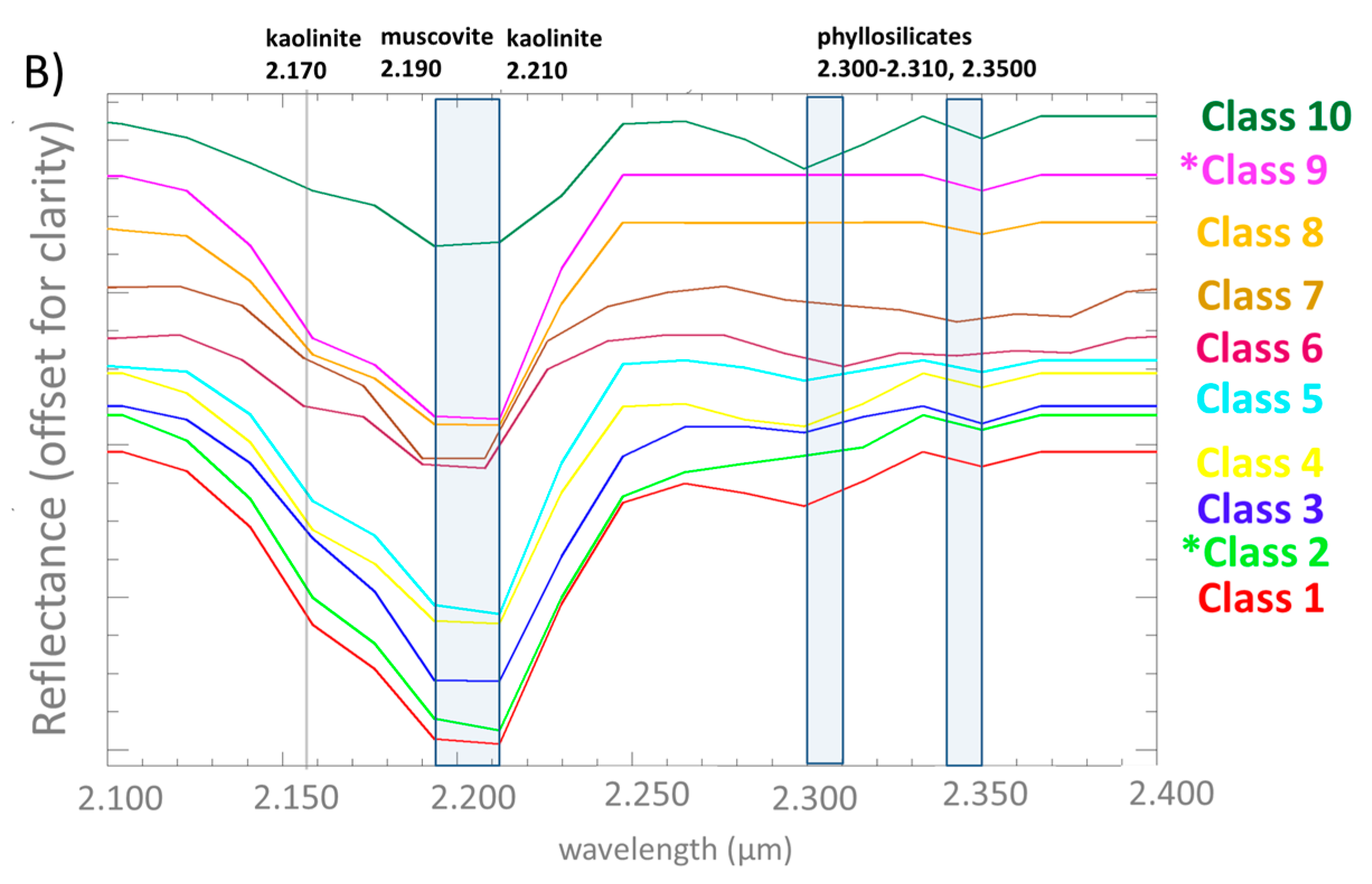
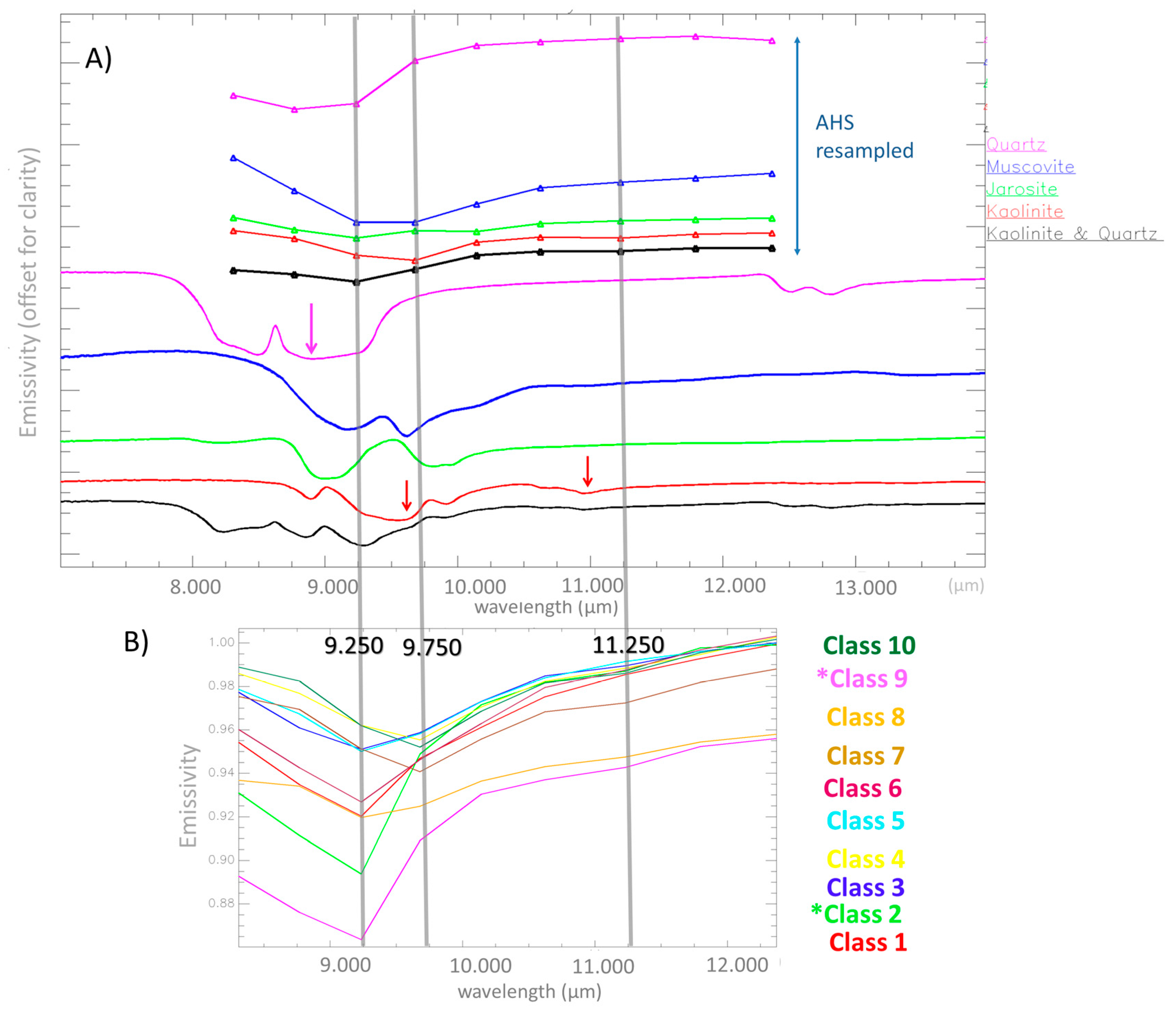
3.2. Linking the Spectral and Mineral Properties

In the VIS/NIR region, the average class spectra (Figure 9A) reflect the variations in absorption features characterising diverse iron oxy-hydroxides (secondary minerals with Fe³⁺) and the organic component (organic C and lignite). Secondary minerals with Fe³⁺ (hydroxysulfates and oxyhydroxides) exhibit absorption features around 0.500 µm and before 1.00 µm [29,69]. The absorption wavelengths and intensities of the absorption features in this region depend on the nature of the crystal field around the Fe atom and on the nature of the bonds around it, because the nature of the magnetic coupling between the Fe³⁺ ions (as influenced by the crystal field) facilitates the transition of electrons between energy states [70]. In addition, shifts in the wavelength positions can also reflect material mixing, when the Fe³⁺ secondary minerals coexist together or with different minerals and an organic component [6]. When interpreting the average class spectra (Figure 9A), it can be seen that Classes 1–3, 5 and 7 exhibit the typical absorption features of secondary Fe³⁺-bearing minerals. The wavelength position of the first absorption shifts from 0.480 to 0.540 µm, while the second one varies between 0.900 and 1.080 nm. The shift of the second absorption indicates that Classes 1–3 represent the lithology where jarosite is present at higher amounts or coexist together with other Fe³⁺-bearing minerals, as jarosite exhibits maximum absorption closer to 0.900 µm (shorter wavelengths). On the other hand, the oxyhydroxides (e.g., goethite and hematite) have the second absorption centred around 1.000 µm (longer wavelengths), therefore this mineral is present at high amounts in Classes 4–7 and 10. The absorptions characteristic of organic C and lignite are at 0.550–0.580 µm and 0.720–0.770 µm, respectively [39], and these two are the most visible in the spectra of Classes 4, 8, 9 and 10.

The overtones and combinations of the fundamental OH and H–O–H vibrations can be mainly observed in the SWIR (Figure 9B). In general, the OH combination bands occur due to the two Al cations in the octahedral sites near 2.210 µm; the spectra of kaolinite shows a distinct absorption doublet at 2.170 and 2.210 µm, whereas muscovite has the main absorption at the shorter wavelength (2.200 µm). The absorption around 2.300 µm characterises carbonates [29]; however, no carbonates were identified at primary, secondary or accessory abundances by the XRD analyses conducted for numerous samples collected in Sokolov. Therefore, in this case, additional smaller absorptions at the longer wavelength (around 2.300 and 2.350 µm) are characteristic of the AlFe–OH and Fe₂–OH combination bands in phyllosilicates [71]. Kaolinite dominates the spectra of Classes 1–2 and 5–6, whereas Classes 3–4 and 7–10 represent mixtures between kaolinite and muscovite as they have less pronounced absorption at 2.170 µm and flat absorption with the same absorption intensities for the wavelength 2.190 and 2.210 µm.

In the LWIR region absorption features, resulting from fundamental molecular vibration modes, show additional information about mineral constituents, such as Si-bearing minerals (mainly quartz and clay minerals). Quartz, due to the molecular vibrations of the Si–O stretching (reststrahlen bands) displays a broad emissivity doublet in the TIR between 8 and 10 µm [72]. In addition, it is possible to differentiate among diverse clay minerals (e.g., kaolinite, illite, and montmorillonite) using the LWIR range [34]. In Figure 10A the emissivity of some silicates is displayed using the Arizona University Spectral library [68], the original emissivity is displayed together with the equivalent emissivity resampled to the spectral resolution of the AHS data. It shows that the AHS data allows quartz, kaolinite or quartz and kaolinite mixtures to be detected. In the case of the AHS data (Figure 10B), quartz affects the emissivity of the bands centred at 9.25 µm (low emissivity) and 9.75 µm (high emissivity) as well as the slope of the emissivity between these two bands. The distinct absorption features detectable by the AHS bands placed at 9.75 µm and 11.2 µm characterise kaolinite. Muscovite exhibits a wide absorption between 9 and 10 µm, and in general lowers the emissivity between 10–12 µm. It can be concluded that Classes 1 and 9 represent lithologies with a dominant quartz content, Classes 1, 2, 5, 6 and 8 then represent a lithology that has both kaolinite and quartz coexisting together. On the other hand, Classes 4, 7 and 10 predominantly have kaolinite.

The classifications (Figure 7 and Figure 8) were compared to the field documentation and XRD analysis of the samples that fall spatially within each class was carried out.

Table 1. Map classes from Figure 7, Figure 8, Figure 9 and Figure 10 compared to the XRD analysis and field documentation of the samples that fall spatially within each class. For Classes 4, 5, 8 and 9 there were no XRD analyses available; however, the mineral description based on the interpretation of the spectral property was added.

Class	Primary Minerals	Secondary and Accessory Minerals	Description	Name
Class 1	kaolinite (60–80%), quartz (up to 10%)	jarosite, hematite, Muscovite, lignite fragments	weathered tuffs on the surface	tuffs
Class 2	quartz > kaolinite	jarosite, hematite, Muscovite	crust developed on the surface of the tuffs	quartz-rich crust
Class 3	kaolinite > quartz	jarosite, hematite, muscovite lignite, pyrite	fresh layer of tuffs exposed by erosion	tuffs
Class 4	kaolinite, quartz, lignite, muscovite		No XRD analysis available	-
Class 5	kaolinite, quarz, hematite, muscovite		No XRD analysis available	-
Class 6	kaolinite	Quartz, muscovite	well-laminated clays with kaolinite content dominating and other admixtures	Cypris clays
Class 7	quartz (>50%), clay content (10–15%)	lignite	back-fill overburden: quartz-rich hard pack with clay matrix, lignite fragments	Back-fill overburden
Class 8	organic C, kaolinite, quartz		no XRD analysis available	soil substrate
Class 9	quartz, kaolinite, lignite, muscovite		no XRD analysis available	-
Class 10	quartz, muscovite, kaolinite	lignite, hematite	weathered Tuffs	tuffs with lignite and hematite

shows the mineralogy (XRD analysis) that characterises six out of 10 defined classes (Classes 1–3, 6, 7 and 10)l for Classes 4, 5, 8 and 9 there were no samples (no XRD analysis) that would fall within their spatial extent. When comparing the mineralogy determined by the XRD with the class spectral properties discussed above, there is good agreement. Kaolinite and quartz represent the dominant minerals for Classes 1–3, whereas jarosite is present together with hematite at secondary abundances, as well as muscovite. However, Class 2 has quartz dominating and was described as a quartz-rich crust developed on the tuffs; on the other hand, Class 3 represents less weathered tuffs exposed by erosion. Class 6 represents the fresh clays of the Cypris formation, where kaolinite is the dominant mineral, followed by quartz and muscovite. Class 7 represents the material of backfill overburden, which was described as quartz-rich hard pack material with a clay matrix also containing lignite fragments. Class 10 represents weathered tuffs in which quartz, muscovite and kaolinite are the dominant, minerals whereas lignite and hematite are present at secondary abundances. Although there were no XRD analyses available for Classes 4, 5, 8 and 9, a mineral description (Table 1) was added; however, it should be emphasised that it is based on the interpretation of the class spectral property (Figure 9 and Figure 10) and in this case it was not possible to differentiate between primary and secondary/accessory abundances of different mineral phases.

4. Discussion

Absorption feature parameters—wavelength position and depth—are the most essential information used in spectroscopy; to put it simply, the maximum absorption wavelength position defines what material it is, whereas absorption depth defines its relative abundance. Different absorption feature mapping/matching techniques have been used by the remote sensing community since hyperspectral data were made available. Among these the spectral feature fitting [73] or its improved version—multi-range spectral feature fitting (MRSFF)—are frequently used [74,75]. From the recently developed toolboxes integrating absorption feature matching techniques the Tetracoder [76] or EnGeoMAP 2.0 toolbox [77] should be listed. These approaches are based on the common principle that they compare and statistically assess the fit of the image spectra to the reference spectra. The reference spectra, called endmembers, are scaled to match the image spectra, and can be either laboratory or field spectral measurements or can be extracted directly from the image (image endmembers). Basically, these classifiers require a routine whereby the endmembers (reference spectra) need to be defined prior to spectral mapping. Moreover, if laboratory or field spectra are used, the successful definition of such endmembers usually requires prior knowledge of the material composition and its spatial distribution within the area of interest. If image endmembers are to be used, and an expert with a background in spectroscopy is required to perform image analysis such as pixel purity analysis (PPI, [78,79]).

In contrast, the approach used here does not require a prior definition of the endmembers or any knowledge of the site conditions; this is a clear advantage. Instead, the absorption wavelength positions and depths of the major absorption features present in different spectral ranges (VNIR/SWIR/LWIR) are extracted automatically and integrated into new raster datasets (multiple absorption feature wavelength and depth matrices). After compressing the main data variability of these new multi-band datasets, using, for instance, an MNF transformation, it is possible to assess the material spatial variability, define training areas (ROIs) and employ a supervised classification. The approach used here is thus unsupervised at the beginning, as no data or knowledge is required prior to absorption feature mapping. Throughout the automatic processing, there is a point where material variability is visualised in a spatial context; afterwards, the training areas (ROIs) for supervised classification are defined. The selection of the spectral ranges under analysis and the definition of the ROIs are the only expert-dependent parts of the analysis. It is thus recommended to divide spectral ranges into VIS/NIR, SWIR and LWIR regions where the diverse mineral groups exhibit distinct absorptions. The definition of the ROIs is rather intuitive as the expert interprets different colour clusters within the image.

Previously, techniques that utilise different types of interpolations for estimating absorption feature wavelength and depth were proposed. Van der Meer [80] proposed a simple linear interpolation technique in order to derive absorption-band position, depth and asymmetry from hyperspectral image. Such parameters were used to interpret the data in terms of the known alteration phases or to estimate heavy metal contents [81]. Rodger et al. [82] proposed a simple quadratic method (SQM) to estimate the wavelengths of absorption features in the shortwave infrared (SWIR) spectral region. The SQM method was tested using spectral data convolved to four different instrument configurations differing in sampling regimes and spectral resolutions. The SQM method was found to estimate feature wavelengths within a reasonable accuracy and to perform well even in noisy environments. Ruitenbeek et al. [83] mapped the wavelength position of the deepest absorption features between 2.100 and 2.400 µm using a second-order polynomial fitting. They concluded that mapping the wavelength position of absorption features between 2.100 and 2.400 µm provided a new method for exploratory analysis of the surface mineralogy and that it would be particularly useful in areas where field validation is sparse and imagery contains shallow spectral absorption features. Moreover, Van der Meer et al. [84] tested two approaches—the ‘Wavelength Mapper’ [83] and the QUANTools [62] (also used for this study)—and demonstrated for the Rodalquilar epithermal system that deriving absorption feature characteristics, such as the wavelength position and the depth, can be directly linked to mineral type and abundance, and, even more, to subtle changes in mineral chemical composition.

However, as seen from the literature, this is the first demonstration of how the multiple absorption features, and their respective parameters, can be extracted automatically from different spectral ranges (VIS/NIR/SWIR and LWIR), and, furthermore, how, when using this rather simple approach, it is possible to successfully ingrate optical (VNIR and SWIR) and thermal (LWIR) spectral information, gathered in this case by two different sensors. It is also demonstrated how further integration can lead to more complex mineral classification. This is a crucial and highly relevant issue nowadays, when, in addition to the optical sensors, the sensors acquiring the data in the LWIR range are more often available and used (e.g., TASI, AISA OWEL) and even more for the future, when a hyperspectral satellite collecting spectral band through the VIS/NIR/SWIR and LWIR will be operating in orbit (e.g., HySPIRI).

So far the different spectral ranges are more frequently analysed and interpreted separately, without combining the full range of information (VIS/NIR/SWIR/LWIR) into a single integrated data product. Too few approaches have been proposed allowing for real optical and thermal data integration; still, they require an expert decision to be made prior to spectral mapping (e.g., endmember definition). As previously explained, the approach used here does not require any prior definition of the endmembers; moreover, there is no need for any knowledge or ground data from the site under study.

In the approach used here, the level of noise present in the image datasets can be a limitation. However, in an example of HyMap VIS/NIR data, it was demonstrated that this problem can be minimised by employing spectral smoothing and that it can be tailored specifically to the level of noise present in the data. In addition, there might be other variables that may create false alarms, such as varying topography causing brightness differences across the image produced by shadow and slope variations, varying mineral particle size and soil moisture content. QUANTools process the data in such a way that at the beginning they are normalised by employing the continuum removal method, which helps to remove the effect of scattering. Then the absorption feature wavelengths are mapped and, as long as the noisy/false absorptions are eliminated, the absorption wavelength positions do not tend to change spectral locations as regards shadows or slope variations. The other absorption feature parameter—absorption depth—reflects the material quantity but is also sensitive to the sizes of mineral particles. Therefore, varying grain size is also part of a final classification. It is thus important to decide if the grain size is also a criterion for material mapping or not. If only the chemical composition of the targets is requested, then it is possible to use only absorption feature wavelength matrices in a classification. In this study, 2010 HyMap and 2011 AHS image data were used to classify two sites, Lítov and Medard, which faced no changes regarding the relief and material transport between 2010 and 2011; however, some differences regarding changes in microtopography or moisture content may have been present. Both absorption feature parameters—wavelength and depth—were used for classifications and brought results that were in good agreement with the XRD analysis, showing that, at a general level, this approach allows diverse minerals to be mapped, including ones that exhibit multiple absorption features though the VIS/NIR/SWIR and LWIR ranges. There are also other useful absorption feature parameters, such as shoulder positions, symmetry or width, that can be used for gathering the information on minor material components, featureless parameters (e.g., heavy metals) or chemical processes/changes. Mapping these additional absorption feature parameters will be a subject for future QUNATools development.

Using this approach, it was possible to integrate the absorption feature information derived from the VIS/NIR/SWIR regions (HyMap data), together with the absorption feature information derived from the LWIR region (AHS data). This integration led to a mineral classification that differentiated between the presence and abundance of diverse Fe³⁺-bearing minerals and phyllosilicates as well as lignite and quartz contents. In addition to HyMap reflectance, the AHS emissivity data allowed a better discrimination between a quartz-dominating crust and substrates (Classes 2 and 9) from the other classes where quartz did not have such dominating abundances and was present together with other mineral phases at primary or secondary abundance (e.g., Classes 1 and 7).

5. Conclusions

In this study, it was demonstrated how the multiple absorption features, respectively their parameters such as wavelengths and depths, can be automatically extracted from different spectral ranges and further integrated into one raster dataset. The absorption feature information gathered from the different spectral-ranges of the two different sensors (HyMap and AHS) was integrated and led to a mineral classification that differentiated between the diverse Fe³⁺-bearing minerals and phyllosilicates as well as lignite and quartz contents and overall resulted in a more complex mineral/lithology classification. This is a crucial and highly relevant issue nowadays, when, in addition to optical sensors, sensors acquiring data in the LWIR range are available and more often used (e.g., TASI, AISA OWEL); and even more for the future, when a hyperspectral satellite collecting a spectral band through the VIS/NIR/SWIR and LWIR will be operating in orbit (e.g., HySPIRI).

It can be concluded that:

• the approach used here does not require prior definition of the endmembers; moreover, there is no need for prior knowledge or data on the specific conditions
• QUANTools, the new toolbox developed, allows automatic and errorless multiple-absorption feature parameters extraction from different spectral ranges, and these parameters can be further integrated into one product, which can consequently be successfully used for mineral mapping/classification
• this multi-range spectral integration leads to more complex mineral/lithology classification
• the approach can be used to integrate the spectral information acquired by different sensors (e.g., HyMap and AHS).

References

1. Van der Meer, F.D.; van der Werff, H.M.; Van Ruitenbeek, F.J.; Hecker, C.A.; Bakker, W.H.; Noomen, M.F.; van der Meijde, M.; Carranza, E.J.M.; De Smeth, J.B.; Woldai, T. Multi-and hyperspectral geologic remote sensing: A review. Int. J. Appl. Earth Obs. Geoinf. 2012, 14, 112–128. [Google Scholar] [CrossRef]
2. Chabrillat, S.; Goetz, A.F.; Krosley, L.; Olsen, H.W. Use of hyperspectral images in the identification and mapping of expansive clay soils and the role of spatial resolution. Remote Sens. Environ. 2002, 82, 431–445. [Google Scholar] [CrossRef]
3. Escribano, P.; Palacios-Orueta, A.; Oyonarte, C.; Chabrillat, S. Spectral properties and sources of variability of ecosystem components in a Mediterranean semiarid environment. J. Arid Environ. 2010, 74, 1041–1051. [Google Scholar] [CrossRef]
4. Haubrock, S.N.; Chabrillat, S.; Kuhnert, M.; Hostert, P.; Kaufmann, H. Surface soil moisture quantification and validation based on hyperspectral data and field measurements. J. Appl. Remote Sens. 2008, 2, 023552. [Google Scholar] [CrossRef]
5. Kokaly, R.F.; Despain, D.G.; Clark, R.N.; Livo, K.E. Mapping vegetation in Yellowstone National Park using spectral feature analysis of AVIRIS data. Remote Sens. Environ. 2003, 84, 437–456. [Google Scholar] [CrossRef]
6. Kopačková, V. Using multiple spectral feature analysis for quantitative pH mapping in a mining environment. Int. J. Appl. Earth Obs. Geoinf. 2014, 28, 28–42. [Google Scholar] [CrossRef]
7. Cudahy, T.; Hewson, R. ASTER geological case histories: Porphyry-skarnepithermal, iron oxide Cu-Au and Broken hill Pb–Zn–Ag. In Proceedings of the Annual General Meeting of the Geological Remote Sensing Group ‘ASTER Unveiled’, London, UK, 6–7 December 2002. [Google Scholar]
8. Kruse, F.A.; Perry, S.L. Mineral mapping using simulated Worldview-3 short-wave-infrared imagery. Remote Sens. 2013, 5, 2688–2703. [Google Scholar] [CrossRef] [Green Version]
9. Van der Meer, F.D.; Van der Werff, H.M.A.; Van Ruitenbeek, F.J.A. Potential of ESA’s Sentinel-2 for geological applications. Remote Sens. Environ. 2014, 148, 124–133. [Google Scholar] [CrossRef]
10. Van der Werff, H.; van der Meer, F. Sentinel-2 for mapping iron absorption feature parameters. Remote Sens. 2015, 7, 12635–12653. [Google Scholar] [CrossRef]
11. Van der Werff, H.; van der Meer, F. Sentinel-2A MSI and Landsat 8 OLI provide data continuity for geological remote sensing. Remote Sens. 2016, 8, 883. [Google Scholar] [CrossRef]
12. Mielke, C.; Boesche, N.K.; Rogass, C.; Kaufmann, H.; Gauert, C.; de Wit, M. Spaceborne mine waste mineralogy monitoring in South Africa, applications for modern push-broom missions: Hyperion/OLI and EnMAP/Sentinel-2. Remote Sens. 2014, 6, 6790–6816. [Google Scholar] [CrossRef]
13. De Morais, M.C.; Junior, P.P.M.; Paradella, W.R. Multi-scale approach using remote sensing images to characterize the iron deposit N1 influence areas in Carajás Mineral Province (Brazilian Amazon). Environ. Earth Sci. 2012, 66, 2085–2096. [Google Scholar] [CrossRef]
14. Khalifa, I.H.; Arnous, M.O. Assessment of hazardous mine waste transport in west central Sinai, using remote sensing and GIS approaches: A case study of Um Bogma area, Egypt. Arabian J. Geosci. 2012, 5, 407–420. [Google Scholar] [CrossRef]
15. Matejicek, L.; Kopackova, V. Changes in croplands as a result of large scale mining and the associated impact on food security studied using time-series Landsat images. Remote Sens. 2010, 2, 1463–1480. [Google Scholar] [CrossRef]
16. Kopačková, V.; Chevrel, S.; Bourguignon, A.; Rojík, P. Application of high altitude and ground-based spectroradiometry to mapping hazardous low-pH material derived from the Sokolov open-pit mine. J. Maps 2012, 8, 220–230. [Google Scholar] [CrossRef]
17. Fernandes, G.W.; Goulart, F.F.; Ranieri, B.D.; Coelho, M.S.; Dales, K.; Boesche, N.; Bustamante, M.; Carvalho, F.A.; Carvalho, D.C.; Dirzo, R.; et al. Deep into the mud: Ecological and socio-economic impacts of the dam breach in Mariana, Brazil. Natureza Conservação 2016, 14, 35–45. [Google Scholar] [CrossRef]
18. Rodríguez-Hernández, A.; Briones-Gallardo, R.; Razo, I.; Noyola-Medrano, C.; Lázaro, I. Processing Methodology Based on ASTER Data for Mapping Mine Waste Dumps in a Semiarid Polysulphide Mine District. Can. J. Remote Sens. 2016, 42, 643–655. [Google Scholar] [CrossRef]
19. Davies, G.E.; Calvin, W.M. Mapping acidic mine waste with seasonal airborne hyperspectral imagery at varying spatial scales. Environ. Earth Sci. 2017, 76, 432. [Google Scholar] [CrossRef]
20. GMES Sentinel-2 Mission Requirements Document. European Space Agency. Available online: http://esamultimedia.esa.int/docs/GMES/Sentinel-2_MRD.pdf (accessed on 1 September 2017).
21. Galeazzi, C.; Sacchetti, A.; Cisbani, A.; Babini, G. The PRISMA program. In Proceedings of the 2008 IEEE International Geoscience and Remote Sensing Symposium, Boston, MA, USA, 6–11 July 2008; Volume 4, p. IV-105. [Google Scholar]
22. Amato, U.; Antoniadis, A.; Carfora, M.F.; Colandrea, P.; Cuomo, V.; Franzese, M.; Pignatti, S.; Serio, C. Statistical classification for assessing PRISMA hyperspectral potential for agricultural land use. IEEE J. Sel. Top. Appl. Earth Obs. Remote Sens. 2013, 6, 615–625. [Google Scholar] [CrossRef]
23. Kaufmann, H.; Segl, K.; Guanter, L.; Hofer, S.; Foerster, K.P.; Stuffler, T.; Mueller, A.; Richter, R.; Bach, H.; Hostert, P.; et al. Environmental mapping and analysis program (EnMAP)-Recent advances and status. In Proceedings of the 2008 IEEE International Geoscience and Remote Sensing Symposium, Boston, MA, USA, 6–11 July 2008; Volume 4, p. IV-109. [Google Scholar]
24. Guanter, L.; Kaufmann, H.; Segl, K.; Foerster, S.; Rogass, C.; Chabrillat, S.; Kuester, T.; Hollstein, A.; Rossner, G.; Chlebek, C.; et al. The EnMAP spaceborne imaging spectroscopy mission for earth observation. Remote Sens. 2015, 7, 8830–8857. [Google Scholar] [CrossRef] [Green Version]
25. Roberts, D.A.; Quattrochi, D.A.; Hulley, G.C.; Hook, S.J.; Green, R.O. Synergies between VSWIR and TIR data for the urban environment: An evaluation of the potential for the Hyperspectral Infrared Imager (HyspIRI) Decadal Survey mission. Remote Sens. Environ. 2012, 117, 83–101. [Google Scholar] [CrossRef]
26. Hunt, G.R. Spectral signatures of particulate minerals in the visible and near infrared. Geophysics 1977, 42, 501–513. [Google Scholar] [CrossRef] [Green Version]
27. Richter, N.; Jarmer, T.; Chabrillat, S.; Oyonarte, C.; Hostert, P.; Kaufmann, H. Free iron oxide determination in Mediterranean soils using diffuse reflectance spectroscopy. Soil Sci. Soc. Am. J. 2009, 73, 72–81. [Google Scholar] [CrossRef]
28. Montero, I.C.; Brimhall, G.H.; Alpers, C.N.; Swayze, G.A. Characterization of waste rock associated with acid drainage at the Penn Mine, California, by ground-based visible to short-wave infrared reflectance spectroscopy assisted by digital mapping. Chem. Geol. 2005, 215, 453–472. [Google Scholar] [CrossRef]
29. Clark, R.N.; King, T.V.; Klejwa, M.; Swayze, G.A.; Vergo, N. High spectral resolution reflectance spectroscopy of minerals. J. Geophys. Res. Solid Earth 1990, 95, 12653–12680. [Google Scholar] [CrossRef]
30. Gobrecht, A.; Roger, J.M.; Bellon-Maurel, V. Major issues of diffuse reflectance NIR spectroscopy in the specific context of soil carbon content estimation: A review. Adv. Agron. 2014, 123, 145–175. [Google Scholar]
31. Sørensen, L.K.; Dalsgaard, S. Determination of clay and other soil properties by near infrared spectroscopy. Soil Sci. Soc. Am. J. 2005, 69, 159–167. [Google Scholar] [CrossRef]
32. Gillespie, A.; Rokugawa, S.; Matsunaga, T.; Cothern, J.S.; Hook, S.; Kahle, A.B. A temperature and emissivity separation algorithm for Advanced Spaceborne Thermal Emission and Reflection Radiometer (ASTER) images. IEEE Trans. Geosci. Remote Sens. 1998, 36, 1113–1126. [Google Scholar] [CrossRef]
33. Van der Meijde, M.; Knox, N.M.; Cundill, S.L.; Noomen, M.F.; Van der Werff, H.M.A.; Hecker, C. Detection of hydrocarbons in clay soils: A laboratory experiment using spectroscopy in the mid-and thermal infrared. Int. J. Appl. Earth Obs. Geoinf. 2013, 23, 384–388. [Google Scholar] [CrossRef]
34. Eisele, A.; Chabrillat, S.; Hecker, C.; Hewson, R.; Lau, I.C.; Rogass, C.; Segl, K.; Cudahy, T.J.; Udelhoven, T.; Hostert, P.; et al. Advantages using the thermal infrared (TIR) to detect and quantify semi-arid soil properties. Remote Sens. Environ. 2015, 163, 296–311. [Google Scholar] [CrossRef]
35. Yitagesu, F.A.; Van der Meer, F.; Van der Werff, H.; Hecker, C. Spectral characteristics of clay minerals in the 2.5–14μm wavelength region. Appl. Clay Sci. 2011, 53, 581–591. [Google Scholar] [CrossRef]
36. Hecker, C.; van der Meijde, M.; van der Meer, F.D. Thermal infrared spectroscopy on feldspars—Successes, limitations and their implications for remote sensing. Earth-Sci. Rev. 2010, 103, 60–70. [Google Scholar] [CrossRef]
37. Horta, A.; Malone, B.; Stockmann, U.; Minasny, B.; Bishop, T.F.A.; McBratney, A.B.; Pallasser, R.; Pozza, L.; et al. Potential of integrated field spectroscopy and spatial analysis for enhanced assessment of soil contamination: A prospective review. Geoderma 2015, 241, 180–209. [Google Scholar] [CrossRef]
38. Vohland, M.; Ludwig, M.; Thiele-Bruhn, S.; Ludwig, B. Determination of soil properties with visible to near-and mid-infrared spectroscopy: Effects of spectral variable selection. Geoderma 2014, 223, 88–96. [Google Scholar] [CrossRef]
39. Kopačková, V.; Ben-Dor, E.; Carmon, N.; Notesco, G. Modelling Diverse Soil Attributes with Visible to Longwave Infrared Spectroscopy Using PLSR Employed by an Automatic Modelling Engine. Remote Sens. 2017, 9, 134. [Google Scholar] [CrossRef]
40. McDowell, M.L.; Kruse, F.A. Enhanced Compositional Mapping through Integrated Full-Range Spectral Analysis. Remote Sens. 2016, 8, 757. [Google Scholar] [CrossRef]
41. Kruse, F.A. Integrated visible and near-infrared, shortwave infrared, and longwave infrared full-range hyperspectral data analysis for geologic mapping. J. Appl. Remote Sens. 2015, 9, 096005. [Google Scholar] [CrossRef]
42. Notesco, G.; Kopačková, V.; Rojík, P.; Schwartz, G.; Livne, I.; Dor, E.B. Mineral classification of land surface using multispectral LWIR and hyperspectral SWIR remote-sensing data. A case study over the Sokolov lignite open-pit mines, the Czech Republic. Remote Sens. 2014, 6, 7005–7025. [Google Scholar] [CrossRef]
43. Feng, J.; Rogge, D.; Rivard, B. Comparison of lithological mapping results from airborne hyperspectral VNIR-SWIR, LWIR and combined data. Int. J. Appl. Earth Obs. Geoinf. 2017, in press. [Google Scholar] [CrossRef]
44. Kruse, F.A.; Lefkoff, A.B.; Boardman, J.W.; Heidebrecht, K.B.; Shapiro, A.T.; Barloon, P.J.; Goetz, A.F.H. The spectral image processing system (SIPS)—Interactive visualization and analysis of imaging spectrometer data. In Proceedings of the AIP Conference Proceedings, St. Louis, MO, USA, 10 August 1993; pp. 192–201. [Google Scholar] [CrossRef]
45. Debba, P.; Van Ruitenbeek, F.J.A.; Van Der Meer, F.D.; Carranza, E.J.M.; Stein, A. Optimal field sampling for targeting minerals using hyperspectral data. Remote Sens. Environ. 2005, 99, 373–386. [Google Scholar] [CrossRef]
46. Haest, M.; Cudahy, T.; Laukamp, C.; Gregory, S. Quantitative mineralogy from infrared spectroscopic data. I. Validation of mineral abundance and composition scripts at the rocklea channel iron deposit in Western Australia. Econ. Geol. 2012, 107, 209–228. [Google Scholar] [CrossRef]
47. Settle, J.J.; Drake, N.A. Linear mixing and the estimation of ground cover proportions. Int. J. Remote Sens. 1993, 14, 1159–1177. [Google Scholar] [CrossRef]
48. Rogge, D.M.; Rivard, B.; Zhang, J.; Feng, J. Iterative spectral unmixing for optimizing per-pixel endmember sets. IEEE Trans. Geosci. Remote Sens. 2006, 44, 3725–3736. [Google Scholar] [CrossRef]
49. Rojík, P. New stratigraphic subdivision of the Tertiary in the Sokolov Basin in Northwestern Bohemia/Nové stratigrafické clenení terciéru sokolovské pánve v sz. Cechách. J. Geosci. 2004, 49, 173. [Google Scholar]
50. Kopačková, V.; Chevrel, S.; Bourguignon, A. Spectroscopy as a tool for geochemical modeling. In Proceedings of the SPIE, Prague, Czech Republic, 19–22 September 2011. [Google Scholar] [CrossRef]
51. Kopačková, V.; Chevrel, S.; Bourguignon, A.; Rojík, P. Mapping hazardous low-pH material in mining environment: Multispectral and hyperspectral aproaches. In Proceedings of the 2012 IEEE International on Geoscience and Remote Sensing Symposium (IGARSS), Munich, Germany, 22–27 July 2012; pp. 2695–2698. [Google Scholar]
52. Götze, C.; Beyer, F.; Gläßer, C. Pioneer vegetation as an indicator of the geochemical parameters in abandoned mine sites using hyperspectral airborne data. Environ. Earth Sci. 2016, 75, 613. [Google Scholar] [CrossRef]
53. Kopačková, V.; Hladíková, L. Applying Spectral Unmixing to Determine Surface Water Parameters in a Mining Environment. Remote Sens. 2014, 6, 11204–11224. [Google Scholar] [CrossRef]
54. Mišurec, J.; Kopačková, V.; Lhotáková, Z.; Hanuš, J.; Weyermann, J.; Entcheva-Campbell, P.; Albrechtová, J. Utilization of hyperspectral image optical indices to assess the Norway spruce forest health status. J. Appl. Remote Sens. 2012, 6, 063545. [Google Scholar]
55. Kopačková, V.; Mišurec, J.; Lhotáková, Z.; Oulehle, F.; Albrechtová, J. Using multi-date high spectral resolution data to assess the physiological status of macroscopically undamaged foliage on a regional scale. Int. J. Appl. Earth Obs. Geoinf. 2014, 27, 169–186. [Google Scholar] [CrossRef]
56. Lhotáková, Z.; Brodský, L.; Kupková, L.; Kopačková, L.; Potůčková, M.; Mišurec, J.; Klement, A.; Kovářová, M.; Albrechtová, J. Detection of multiple stresses in Scots pine growing at post-mining sites using visible to near-infrared spectroscopy. Environ. Sci. Process. Impacts 2013, 15, 2004–2015. [Google Scholar]
57. Richter, R.; Schläpfer, D. Geo-atmospheric processing of airborne imaging spectrometry data. Part 2: Atmospheric/topographic correction. Int. J. Remote Sens. 2002, 23, 2631–2649. [Google Scholar] [CrossRef]
58. Adler-Golden, S.M.; Matthew, M.W.; Bernstein, L.S.; Levine, R.Y.; Berk, A.; Richtsmeier, S.C.; Acharya, P.K.; Anderson, G.P.; Felde, J.W.; Gardner, J.A.; et al. Atmospheric correction for short-wave spectral imagery based on MODTRAN 4. In Proceedings of the International Society for Optical Engineering, Denver, CO, USA, 21–22 July 1999. [Google Scholar]
59. Adar, S.; Shkolnisky, Y.; Notesco, G.; Ben-Dor, E. Using Visible Spectral Information to Predict Long-Wave Infrared Spectral Emissivity: A Case Study over the Sokolov Area of the Czech Republic with an Airborne Hyperspectral Scanner Sensor. Remote Sens. 2013, 5, 5757–5782. [Google Scholar] [CrossRef]
60. Miguel, E.D.; Jiménez, M.; Pérez, I.; Cámara, Ó.G. AHS and CASI processing for the REFLEX remote sensing campaign: Methods and results. Acta Geophys. 2015, 63, 1485–1498. [Google Scholar] [CrossRef]
61. Yuan, H.; Bish, D.L. NEWMOD+, a new version of the NEWMOD program for interpreting X-ray powder diffraction patterns from interstratified clay minerals. Clays Clay Miner. 2010, 58, 318–326. [Google Scholar] [CrossRef]
62. Kopačková, V.; Koucká, L. Mineral Mapping Based on Automatic Detection of Multiple Absorption Features. Available online: http://www.eproceedings.org/static/vol13_S1/13_S1_kopackova2.pdf (accessed on 3 September 2017).
63. Clark, R.N.; Roush, T.L. Reflectance spectroscopy: Quantitative analysis techniques for remote sensing applications. J. Geophys. Res. Solid Earth 1984, 89, 6329–6340. [Google Scholar] [CrossRef]
64. Green, A.A.; Berman, M.; Switzer, P.; Craig, M.D. A transformation for ordering multispectral data in terms of image quality with implications for noise removal. IEEE Trans. Geosci. Remote Sens. 1988, 26, 65–74. [Google Scholar] [CrossRef]
65. Richards, J.A. Remote Sensing Digital Image Analysis; Springer: Berlin, Germany, 1999; Volume 3. [Google Scholar]
66. Hudak, A.T.; Brockett, B.H. Mapping fire scars in a southern African savannah using Landsat imagery. Int. J. Remote Sens. 2004, 25, 3231–3243. [Google Scholar] [CrossRef]
67. Manzo, C.; Mei, A.; Salvatori, R.; Bassani, C.; Allegrini, A. Spectral modelling used to identify the aggregates index of asphalted surfaces and sensitivity analysis. Constr. Build. Mater. 2014, 61, 147–155. [Google Scholar] [CrossRef]
68. The Spectral Library Hosted by the Mars Space Flight Facility at Arizona State University. Available online: http://speclib.asu.edu (accessed on 20 May 2017).
69. Murphy, R.J.; Monteiro, S.T. Mapping the distribution of ferric iron minerals on a vertical mine face using derivative analysis of hyperspectral imagery (430–970nm). ISPRS J. Photogramm. Remote Sens. 2013, 75, 29–39. [Google Scholar] [CrossRef]
70. Sherman, D.M.; Waite, T.D. Electronic spectra of Fe3+ oxides and oxide hydroxides in the near IR to near UV. Am. Mineral. 1985, 70, 1262–1269. [Google Scholar]
71. Bishop, J.L.; Lane, M.D.; Dyar, M.D.; Brown, A.J. Reflectance and emission spectroscopy study of four groups of phyllosilicates: Smectites, kaolinite-serpentines, chlorites and micas. Clay Miner. 2008, 43, 35–54. [Google Scholar] [CrossRef]
72. Salisbury, J.W.; D’Aria, D.M. Emissivity of terrestrial materials in the 8–14 μm atmospheric window. Remote Sens. Environ. 1992, 42, 83–106. [Google Scholar] [CrossRef]
73. Clark, R.N.; Swayze, G.A.; Gallagher, A.; Gorelick, N.; Kruse, F.A. Mapping with imaging spectrometer data using the complete band shape least-squares algorithm simultaneously fit to multiple spectral features from multiple materials. In Proceedings of the Third Airborne Visible/Infrared Imaging Spectrometer (AVIRIS) Workshop; Jet Propulsion Laboratory: La Cañada Flintridge, CA, USA, 1991; Volume 42, pp. 2–3. [Google Scholar]
74. Pan, Z.; Huang, J.; Wang, F. Multi range spectral feature fitting for hyperspectral imagery in extracting oilseed rape planting area. Int. J. Appl. Earth Obs. Geoinf. 2013, 25, 21–29. [Google Scholar] [CrossRef]
75. Shanmugam, S.; SrinivasaPerumal, P. Spectral matching approaches in hyperspectral image processing. Int. J. Remote Sens. 2014, 35, 8217–8251. [Google Scholar] [CrossRef]
76. Clark, R.N.; Swayze, G.A.; Livo, K.E.; Kokaly, R.F.; Sutley, S.J.; Dalton, J.B.; McDougal, R.R.; Gent, C.A. Imaging spectroscopy: Earth and planetary remote sensing with the USGS Tetracorder and expert systems. J. Geophys. Res. Planets 2003. [Google Scholar] [CrossRef]
77. Mielke, C.; Rogass, C.; Boesche, N.; Segl, K.; Altenberger, U. EnGeoMAP 2.0—Automated hyperspectral mineral identification for the german EnMAP space mission. Remote Sens. 2016, 8, 127. [Google Scholar] [CrossRef]
78. Boardman, J.W.; Kruse, F.A. Automated spectral analysis: A geological example using AVIRIS data, north Grapevine Mountains, Nevada. In Proceedings of the Thematic Conference on Geologic Remote Sensing, San Antonio, TX, USA, 9–12 May 1994; p. I-407. [Google Scholar]
79. Kruse, F.A.; Richardson, L.L.; Ambrosia, V.G. Techniques Developed for Geologic Analysis of Hyperspectral Data Applied to Near-Shore Hyperspectral Ocean Data. Available online: http://ww.w.hgimaging.com/PDF/Kruse_erim97_marine.pdf (accessed on 3 September 2017).
80. Van Der Meer, F. Analysis of spectral absorption features in hyperspectral imagery. Int. J. Appl. Earth Obs. Geoinf. 2004, 5, 55–68. [Google Scholar] [CrossRef]
81. Choe, E.; van der Meer, F.; van Ruitenbeek, F.; van der Werff, H.; de Smeth, B.; Kim, K.W. Mapping of heavy metal pollution in stream sediments using combined geochemistry, field spectroscopy, and hyperspectral remote sensing: A case study of the Rodalquilar mining area, SE Spain. Remote Sens. Environ. 2008, 112, 3222–3233. [Google Scholar] [CrossRef]
82. Rodger, A.; Laukamp, C.; Haest, M.; Cudahy, T. A simple quadratic method of absorption feature wavelength estimation in continuum removed spectra. Remote Sens. Environ. 2012, 118, 273–283. [Google Scholar] [CrossRef]
83. Van Ruitenbeek, F.J.; Bakker, W.H.; van der Werff, H.M.; Zegers, T.E.; Oosthoek, J.H.; Omer, Z.A.; Marsh, S.H.; van der Meer, F.D. Mapping the wavelength position of deepest absorption features to explore mineral diversity in hyperspectral images. Planet. Space Sci. 2014, 101, 108–117. [Google Scholar] [CrossRef]
84. Van der Meer, F.D.; Kopackova, V.; Koucká, L.; van der Werff, H.M.; van Ruitenbeek, F.J.; Bakker, W.H. Wavelength feature mapping as a proxy to mineral chemistry for investigating geologic systems: An example from the Rodalquilar epithermal system. Int. J. Appl. Earth Obs. Geoinf. 2017. in print. [Google Scholar]
Figure 1. Geographic position of the two sites under study: Lítov dump and Medard Lake, Sokolov basin, Czech Republic.
Remotesensing 09 01006 g001
Figure 2. QUANTools: a simplified processing scheme (CR: continuum removal, λ : wavelength loc_mac: local absorption feature maximum). The detected absorption feature parameters are sorted in ascending order by wavelength ( λ 1 , λ 2   λ z ) .
Remotesensing 09 01006 g002
Figure 3. Bad band detection (spectral range 0.450–1.200 µm) in QuanTools where the bad bands detected are shown by the green square points and the corrected curve as a dashed line (set spectral window: three neighbouring bands).
Remotesensing 09 01006 g003
Figure 4. Scheme of the processing allowing integration of the absorption feature information detected in VIS/NIR/SWIR and LWIR data and further classification.
Remotesensing 09 01006 g004
Figure 5. Lítov: MNF1/MNF2/MNF3 images displayed as RGB: (A) Scenario 1 (absorption feature parameters derived only from the HyMap data were used); (B) Scenario 2 (absorption feature parameters derived from both datasets, HyMap and AHS, were used), the MNF bands were further visually analysed to identify training areas (ROIs) representing different material/surfaces.
Remotesensing 09 01006 g005
Figure 6. The manually derived absorption wavelength positions from 50 different image pixels of the the HyMap and the AHS image data representing different material/surfaces compared to the absorption wavelength positions derived automatically when using QaunTools.
Remotesensing 09 01006 g006
Figure 7. Lítov, mineral mapping: (A) orthophoto showing the Lítov dump; (B) classification using Scenario 1 (absorption feature parameters derived only from the HyMap data were used for the consequent mineral mapping), (C) classification using Scenario 2 (absorption feature parameters derived from both datasets, HyMap and AHS, were used for the consequent mineral mapping), (D) enlargement of the area of interest. The mapped classes correspond to the mineral classes in Table 1, *Class 2 and *Class 9: two additional classes mapped when using Scenario 2.
Remotesensing 09 01006 g007
Figure 8. Medard Lake, mineral mapping: (A) orthophoto showing the Lítov dump, (B) classification using Scenario 1 (absorption feature parameters derived only from the HyMap data were used for the consequent mineral mapping), (C) classification using Scenario 2 (absorption feature parameters derived from both datasets, HyMap and AHS, were used for the consequent mineral mapping), (D) enlargement of the area of interest. The mapped classes correspond to the mineral classes in the Table 1, *Class 2 and *Class 9: two additional classes mapped when using Scenario 2.
Remotesensing 09 01006 g008
Figure 9. The average class spectrum derived from the HyMap data: (A) the VIS/NIR spectral range (0.450–1.200 µm); (B) the SWIR range (2.100–2.400 µm).
Remotesensing 09 01006 g009aRemotesensing 09 01006 g009b
Figure 10. (A) Emissivity of some silicates is displayed using the Arizona University Spectral library [68], the original spectra are displayed together with the equivalent spectra resampled to the spectral resolution of the AHS data. (B) The average class spectrum derived from the AHS data. The mapped classes correspond to the mineral classes in Table 1, *Class 2 and *Class 9: two additional classes mapped when using Scenario 2.
Remotesensing 09 01006 g010