Pointing Verification Method for Spaceborne Lidars

Abstract

High precision acquisition of atmospheric parameters from the air or space by means of lidar requires accurate knowledge of laser pointing. Discrepancies between the assumed and actual pointing can introduce large errors due to the Doppler effect or a wrongly assumed air pressure at ground level. In this paper, a method for precisely quantifying these discrepancies for airborne and spaceborne lidar systems is presented. The method is based on the comparison of ground elevations derived from the lidar ranging data with high-resolution topography data obtained from a digital elevation model and allows for the derivation of the lateral and longitudinal deviation of the laser beam propagation direction. The applicability of the technique is demonstrated by using experimental data from an airborne lidar system, confirming that geo-referencing of the lidar ground spot trace with an uncertainty of less than 10 m with respect to the used digital elevation model (DEM) can be obtained.

1. Introduction

Active optical remote sensing of atmospheric parameters or constituents from spaceborne platforms is increasingly attracting attention. The advantages over passive sensors, such as independence from daytime and nighttime conditions or the seasons and reduced sensitivities to aerosols [1] in case of trace gas soundings were hampered by technical challenges for a long time. The measurement sensitivities of existing passive sensors have already achieved results in demanding technical requirements for future active systems. Nowadays, ongoing technical progress has brought active sensors within reach of feasibly exceeding the performances of passive sensors.

First, active optical systems for measuring atmospheric parameters or constituents have already been in operation successfully on space platforms [2,3,4] or are being planned [5,6,7,8,9].

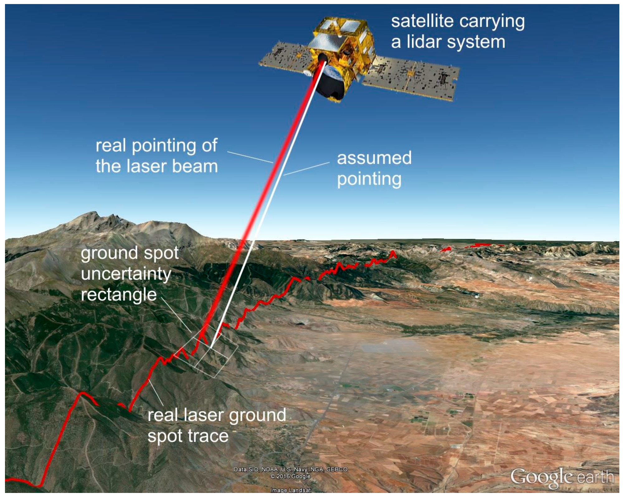
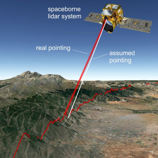
For the sounding of atmospheric trace gases using lidars (light detection and ranging), it is of paramount importance to have accurate knowledge about the lidar pointing angles from the satellite to the Earth’s surface (see Figure 1). For the DIAL (differential absorption lidar [10]) or the IPDA-lidar (integrated path differential absorption lidar [11]) methods, two factors play an important role: First, any deviation from an optimized angle between the directional vector of the platform motion and the laser beam cause undesired Doppler shifts on the measurement wavelengths. Those have to be precisely known and considered during the data retrieval. Second, the air pressure profile along the laser beam, i.e., along the measured atmospheric volume, has to be precisely determined. In particular, in the case of IPDA-lidars, retrieving the total trace gas column, the knowledge of the air pressure on the ground, and thus, the laser ground spot elevation is required to be known with high accuracy. This implies a precise knowledge of the lidar pointing.

Satellite platforms provide data about their attitude angles, retrieved by onboard systems, such as star trackers [12]. However, high accuracy demands costly systems. A reasonable cost-benefit calculation has to be made for each mission. Additionally, it cannot be excluded that these systems do not provide exactly the needed information, for example, if thermo-elastic effects along the orbit affect the lidar pointing. Especially in the case of scanning systems, the assumed beam pointing implicates uncertainties since scanning devices are also subject to limitations in terms of positioning knowledge. Consequently, a verification of the available pointing data using an independent reference is required as well as a quantification in case deviations occur, so that a correction can be performed.

The requirements depend strongly on the purpose and type of the lidar system. For example, for spaceborne CO₂ measurements, severe pointing knowledge stabilities of 66 μrad were specified to be met for a sufficient consideration of the Doppler shift (with respect to the measurement error budget) in the framework of the A-SCOPE studies (advanced space carbon and climate observation of planet earth) [11,13,14]. In case of CH₄ soundings, error budget analyses for the MERLIN mission (methane remote sensing lidar mission) [5,6] imply relaxed pointing stability requirements on the order of 400 μrad [15] due to the spectral properties of methane in the 1.64 μm spectral domain [16].

In this paper, an approach for the quantification of lidar pointing deviations from the assumed pointing is described and demonstrated by using experimental data from airborne measurements. Furthermore, the sensitivity of the method is investigated and discussed.

2. Method

The intrinsic ranging capability of airborne or spaceborne lidar systems operating with short laser pulses (in the ns to μs range) results in spatially high resolved data sets of the distance between the instrument and the ground along the flight path. These distance profiles along the path are determined by the flight altitude of the platform and the laser pointing (described by roll = rotation around the longitudinal axis and pitch = rotation around the lateral axis). The flight altitude, the pointing angles, the measured distance to the ground and the ground elevation represent a self-contained and consistent data set for each lidar measurement point. Each quantity can be calculated from the remaining ones. The flight altitude, obtained from GPS data (global positioning system), and the lidar ranging to the ground (obtained from the laser pulse runtime measurement) are typically known with at least a few meters uncertainty. High-precision ground elevation data are available with resolutions of about 15 m (vertically) and 25 m (horizontally) or better.

Airborne or spaceborne lidar systems acquire a huge amount of ranging data during their measurements containing the surface topography fingerprint. The question is: to what extent is it possible to derive the pointing angles using these ranging data in terms of angle resolution? This issue was investigated in this study by the application of real lidar ranging data obtained during airborne measurements performed with the greenhouse gas lidar CHARM-F (CO₂ and CH₄ remote monitoring—Flugzeug) on the German research aircraft HALO (high altitude and long range research aircraft) in 2015 (for system parameters, see

Table 1. CHARM-F’s main system parameters.

Parameter	Value
Lidar type	Integrated path differential absorption (IPDA) lidar
Laser wavelengths	1.572 μm (CO2), 1.646 μm (CH4)
Laser systems	Optical parametric oscillators (OPO) pumped by Nd:YAG lasers
Laser power	10 mJ per pulse
Laser pulse repetition rate	50 Hz (double pulses)
Laser pulse width	20 ns
Detector types	InGaAs photo diodes
Detection chain bandwidth	3 MHz
Receiver telescopes field of view	3.3 mrad (full angle)
Laser spot on ground	max. 50 m Ø, typ. 25 m–40 m Ø
Ranging precision	<0.25 m (1σ)
Ranging accuracy	<5 m

).

The terrain elevation information along the laser ground spot trace represents a unique pattern (assuming an adequately structured terrain), which allows an a posteriori matching of the lidar elevation data with available terrain elevation data from other sources.

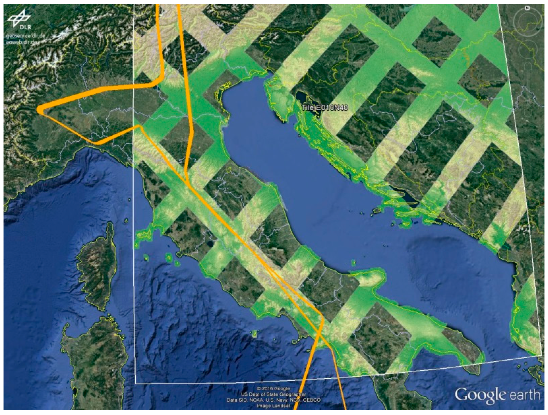
In this study, high-resolution DEM (digital elevation model) data from SRTM/X-SAR (shuttle radar topography mission/X-band synthetic aperture radar) were used for the matching (© DLR/ASI 2010) [17]. The data do not cover the complete surface of the Earth, but are available in stripes. In Central Italy, such a stripe matches our flight path along a mountainous region (see Figure 2). The pixel size of the DEM data is 1” × 1” (in latitude and longitude), and so about 30 m (latitude) × 23 m (longitude) in that area. The horizontal accuracy of the data is specified to be ±20 m (absolute) and ±15 m (relative), the vertical accuracy ±16 m (absolute) and ±6 m (relative). The CHARM-F data have a spatial resolution of 4 m along the flight path (i.e., single measurement points are overlapping due to the laser ground spot diameter of about 25 m). A data averaging of the lidar data was not performed.

For quantifying the degree of the matching, the linear (Pearson) correlation coefficients r between the measured lidar ground elevations x_i and the DEM data y_i for defined sections of the flight track (with n lidar measurement points and i as the point number) are calculated as indicated in Equation (1).

$$r_{xy}=\frac{n{\displaystyle {\sum }_{i=1}^n\left(x_i·y_i\right)-\left({\displaystyle {\sum }_{i=1}^n{x}_i}\right)·\left({\displaystyle {\sum }_{i=1}^n{y}_i}\right)}}{\sqrt{\left(n{\displaystyle {\sum }_{i=1}^n{x}_i^2}-{\left({\displaystyle {\sum }_{i=1}^n{x}_i}\right)}^2\right)·\left(n{\displaystyle {\sum }_{i=1}^n{y}_i^2}-{\left({\displaystyle {\sum }_{i=1}^n{y}_i}\right)}^2\right)}}$$

(1)

The data from the onboard aircraft attitude acquisition systems are taken as the a priori information to initiate the search for the real laser ground spot positions (“initial values”). The laser ground spot positions trace (considering all aircraft movements) is calculated using: 1. the aircraft’s GPS positions; 2. the aircraft’s flight altitudes; 3. the aircraft’s roll, pitch, and yaw angles and 4. the lidar ranging information. This results in a series of latitudes, longitudes, and SSEs (surface scattering elevations, i.e., the corresponding elevations of the lidar ground spot return signals) along the flight track. The geolocation data (latitude and longitude) of the calculated lidar ground spot trace are used to pick out the ground elevation data from the DEM.

The presented approach to detect and determine existing deviations from the assumed pointing angles (pitch and roll) is based on the calculation of the correlation coefficients (for DEM and lidar SSE data) for pitch and roll variations around the initially available pitch and roll values (= “assumed ground spot trace”).

First, a fixed interval of lidar SSE data (“check interval”), i.e., a suitable flight path section, is chosen such that it shows significant variability in terms of surface topography. The angle deviations to be determined are assumed constant within this interval. Then, the correlation coefficients between the lidar SSEs and the DEM elevations are calculated for this fixed interval according to Equation (1) and are arranged in a 2-D array corresponding to a stepwise variation of pitch and roll angles. The size of the array is determined by the chosen variation resolution and the expected deviation range from the initial values. The global maximum in this correlation array corresponds to the best match of the lidar ground spot SSE trace with the existing surface topography, represented by the DEM. Hence, the corresponding pair of pitch and roll angles specifies the deviation of the actual laser pointing from the assumed pointing. All given values for pitch and roll in this paper are related to an aircraft altitude of 9000 m, whereas all given horizontal shifts or deviations on the ground do not depend on the flight altitude.

3. Results

For demonstration purposes, the described procedure was applied using CHARM-F flight measurements obtained over the Apennine Mountains (Central Italy), which can be characterized as a low mountain range. This kind of topography turned out to be a suitable area for lidar pointing verifications and quantifications, because of its information density and information uniqueness, as well as the fact that the SAR data are without gaps thanks to the moderate slopes of those mountains.

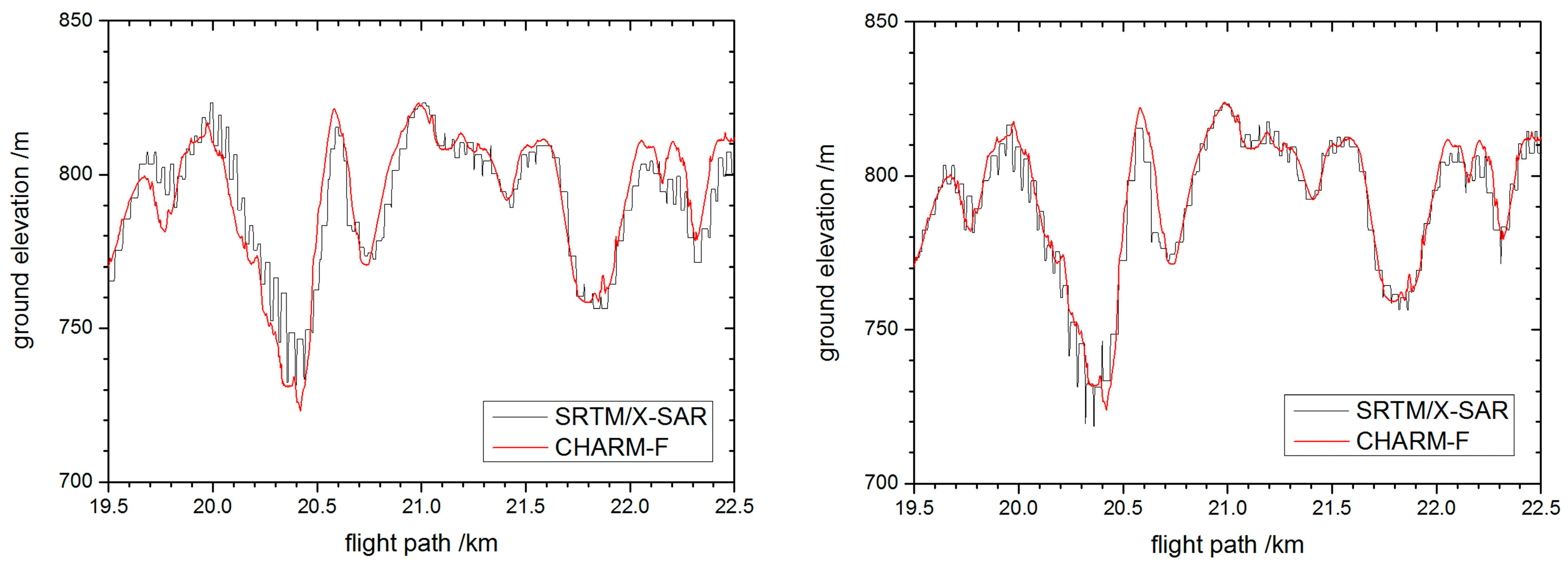
Figure 3 shows a direct comparison of the lidar SSE data with the DEM data for the assumed lidar ground spot locations based on the lidar ranging and available attitude data. The plot (left panel) shows good agreement between DEM and the CHARM-F lidar (correlation coefficient: 0.969). It has to be stressed that in this plot, elevation data from two very different sources are brought together without any further adaptions, using only their geo-referenced coordinates. Nevertheless, it turned out that it is possible to achieve an even better agreement between DEM and lidar, if the assumed lidar ground spot trace is slightly shifted by adjusting the given roll and pitch angles, i.e., by correcting the pointing information. A roll offset of −0.09° (≈13 m lateral shift on the ground) and a pitch offset of +0.12° (≈17 m longitudinal shift on the ground) leads to the plot in the right panel of Figure 3 (correlation coefficient: 0.989). Such offsets can be caused by the actual laser pointing adjustment of the instrument and/or by uncertainties of the attitude acquisition system of the aircraft. The values are well within the expected range and they are consistent along the flight section (see below). This example clearly illustrates the high sensitivity of the method and the calculability of the offsets.

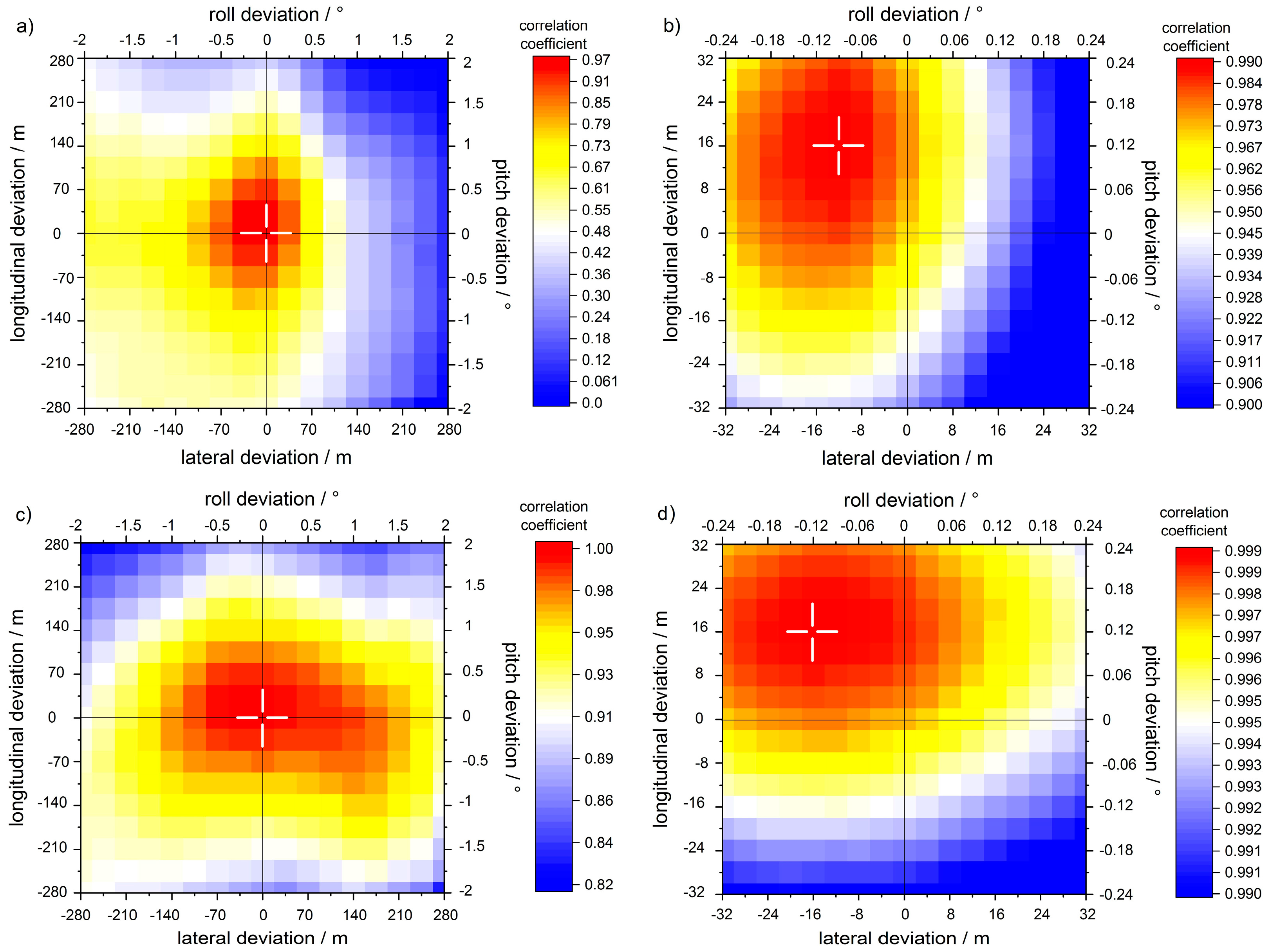
For testing purposes, 10 consecutive check intervals with 1000 lidar measurement points each (i.e., 4 km length) were analyzed. For two of them the resulting correlation arrays are visualized in Figure 4. The centers of the plots correspond to the initially assumed ground spot trace (i.e., assumed pointing angle pair). On the left hand side the arrays are shown for spatial deviations of up to 280 m (35 m per pixel) and on the right hand side zooms are plotted with deviations of up to 32 m (4 m per pixel). The white cross depicts the pitch and roll angle pair, for which the highest correlation between lidar data and DEM was found. For all tested cases, the values in the array around the maximum are strictly monotonic, increasing in both dimensions towards one point of maximum correlation. The resulting offsets were found to be consistent for the 10 consecutive test sections showing a maximum variation of 6 m from their mean, which is well below both the laser ground spot diameter and the horizontal resolution of the DEM. Note that this value is also increased by the spatial uncertainty of the DEM pixel allocation (relative to each other).

The optimal length of the check interval depends on the present topography and the actual pointing deviation. For large pointing deviations, lidar and SRTM elevations can become uncorrelated for certain lengths of the check interval (e.g., >2° roll deviation for the test section no. 1 shown above). For those cases, longer check intervals help to achieve significant correlation coefficients again, since terrain structures on larger scales can contribute to the calculation.

Figure 5 shows an example for stronger deviations from the true pointing along with the application of an extended check interval of 8 km. Here, a pitch offset of 3.5° (≈500 m longitudinal shift on the ground) and a roll offset of 3.5° (≈500 m lateral shift on the ground) result in a correlation coefficient of 0.819. Therefore, the length of the check interval has to be adjusted to the expected deviations, depending on the characteristic of the topography inside the check interval, to get an optimal performance of this method. Further tests on the available data show that the consistency of the pointing determination for consecutive check intervals (i.e., the achieved pointing angle determination precision) can be increased by using longer check intervals.

For information: For the 10 test sections discussed above, the optimized lidar ground spot traces lead to elevation differences between lidar and DEM between 3.1 m and 5.5 m (mean absolute deviations) with standard deviations of the elevation differences (DEM minus lidar using single lidar shots) between 4.2 m and 6.8 m.

4. Discussion

The results shown in the previous section indicate that this method is mainly limited by the precision and accuracy of the used data, as long as a sufficient number of lidar measurements in combination with an appropriate length of the check interval is chosen for the analysis.

The calculation of correlation coefficients is obvious for this kind of objective, but is not the only way to quantify the degree of the matching; the results show the effectiveness, but the required computing time is long. For example, adding up the point-to-point differences of DEM elevations minus lidar elevations along the check interval could reduce the computing time and give useful values as well. The performance of this or of similar simpler calculations was not tested in this study in detail.

Transferring the results presented above to satellite geometries, the pointing angle determination sensitivity is increased due to the higher distance to the ground. However, a lower spatial resolution of the lidar ranging data on the ground has to be assumed, because of the larger laser ground spot diameter. Assuming a LEO (low earth orbit) satellite carrying a lidar with an orbit altitude of 500 km (i.e., 50 times higher angle resolution) and a laser ground spot diameter of 150 m (i.e., 6 times lower spatial resolution on the ground), a pointing angle sensitivity of about 0.007° (120 μrad) can be estimated (assuming a 60 m ground spot trace geolocation uncertainty, resulting from a decreased lidar-DEM matching precision, conservatively estimated). The check interval would be longer, because of the fast ground speed of a LEO satellite (e.g., 360 km length for 1000 measurement points, assuming 7.2 km/s speed and 20 Hz laser repetition rate). This means the required pointing stability for the MERLIN lidar can be verified by this method using the above mentioned parameters. It can be assumed that the application of a DEM with higher spatial precision and accuracy than the SRTM-DEM in combination with an appropriate amount of lidar measurements can lead to even better performances of the presented method.

5. Conclusions

This paper describes a method for the determination of lidar pointing angle deviations from the assumed pointing for airborne or spaceborne systems and discusses its sensitivity. It is based on the matching of lidar ground spot elevation data, obtained from the lidar ranging, with ground elevation data from a digital elevation model.

The approach is to calculate a correlation coefficient array, resulting from a (sufficiently wide) stepwise variation of pitch and roll angles around the initially assumed lidar pointing. This results in a unique optimum (i.e., a pair of pitch and roll values), representing the best match between lidar and DEM along a chosen check interval, thus specifying the real pointing angles. The length of the check interval on the ground and the number of the applied lidar measurements have to be adapted in order to achieve appropriate correlation coefficients and precise results. In addition, the expected pointing deviations as well as the required pointing sensitivity have to be considered. The topography of low mountain ranges was found to be suitable for this kind of analysis.

Applying the method on airborne lidar measurements, a geo-referencing of the lidar ground spot trace with uncertainties of below 10 m related to the DEM used (SRTM/X-SAR) was reached. 1000 lidar measurement points compared with DEM data are sufficient for stable results. Thus, the achieved uncertainty was mainly limited by the spatial accuracy and precision of the DEM.

This means that for airborne lidar systems (e.g., with flight altitudes of 9000 m, as in the case presented here) that the pointing can be determined with uncertainties of below 0.05° (related to the DEM used). For spaceborne lidar systems, e.g., on LEO satellites with a 500 km orbit altitude, the angle sensitivity is correspondingly improved to about 0.007° (120 μrad). For instance, this is below the required pointing stability specified for the MERLIN lidar instrument. Hence, this technique allows for a reliable verification of its pointing. Even higher angle resolutions can be expected from using DEMs with correspondingly high precision and accuracy as well as an appropriately adapted amount of lidar measurement points.