
Estimating the Biomass of Maize with Hyperspectral and LiDAR Data


Abstract
:
1. Introduction
2. Materials
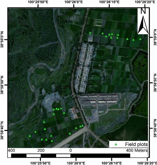
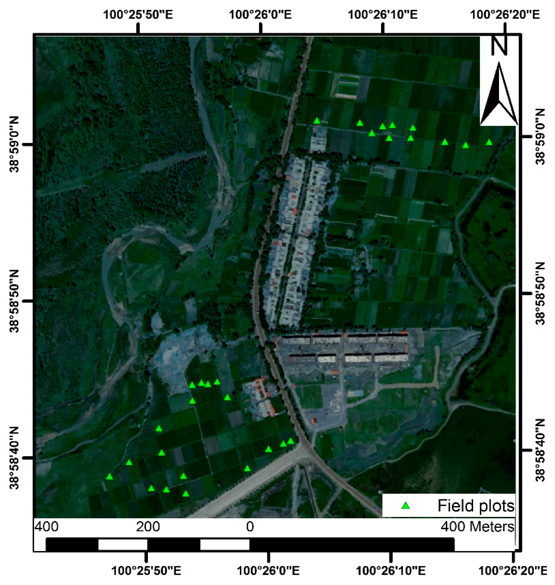
2.1. Study Area
2.2. Airborne LiDAR Data
2.3. Airborne Hyperspectral Data
2.4. Field Measurement
3. Methods
3.1. Deriving Metrics from Hyperspectral Data
3.2. Deriving Metrics from LiDAR
3.3. Regression Analysis
4. Results
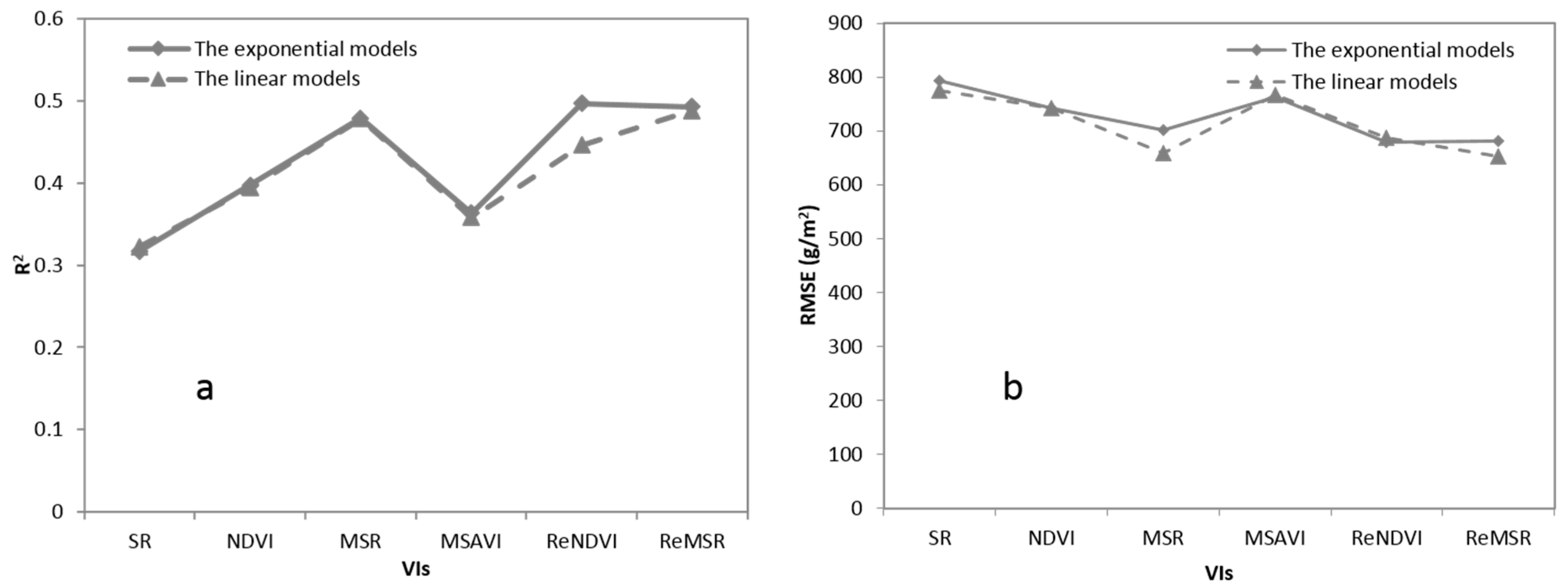
4.1. VIs as Predictors of Vegetation Biomass
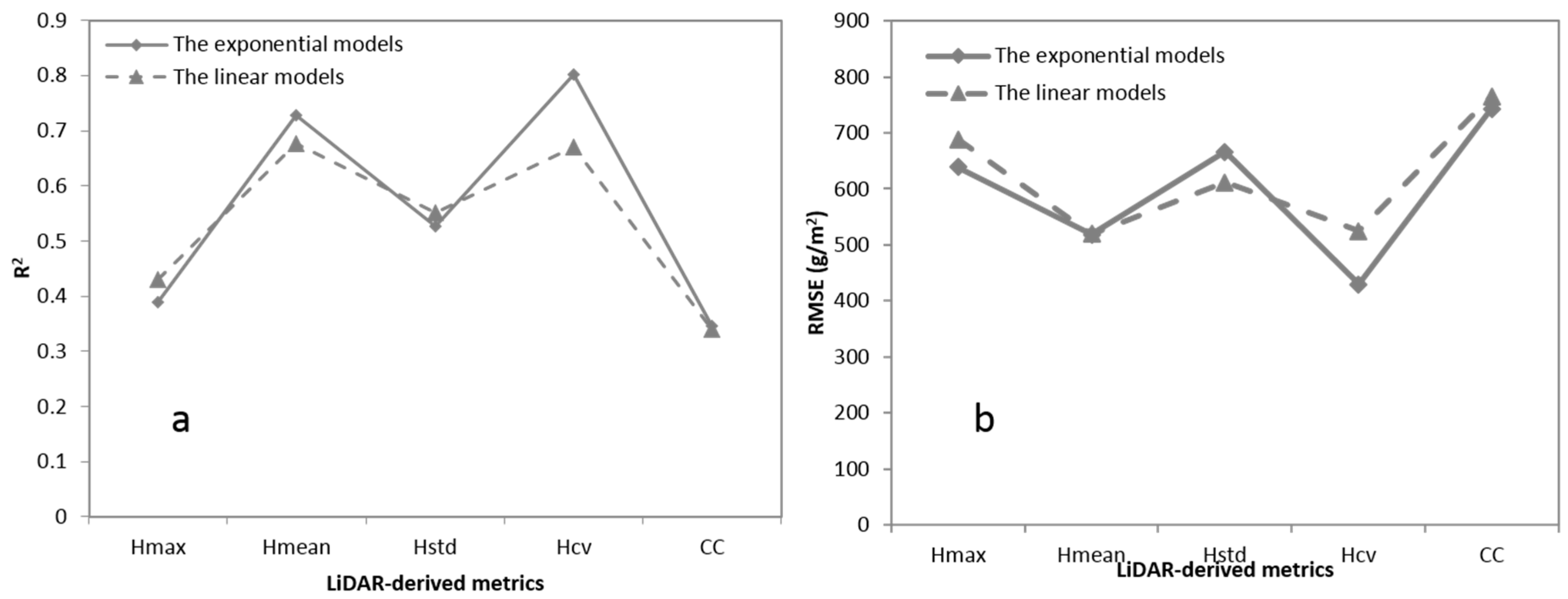
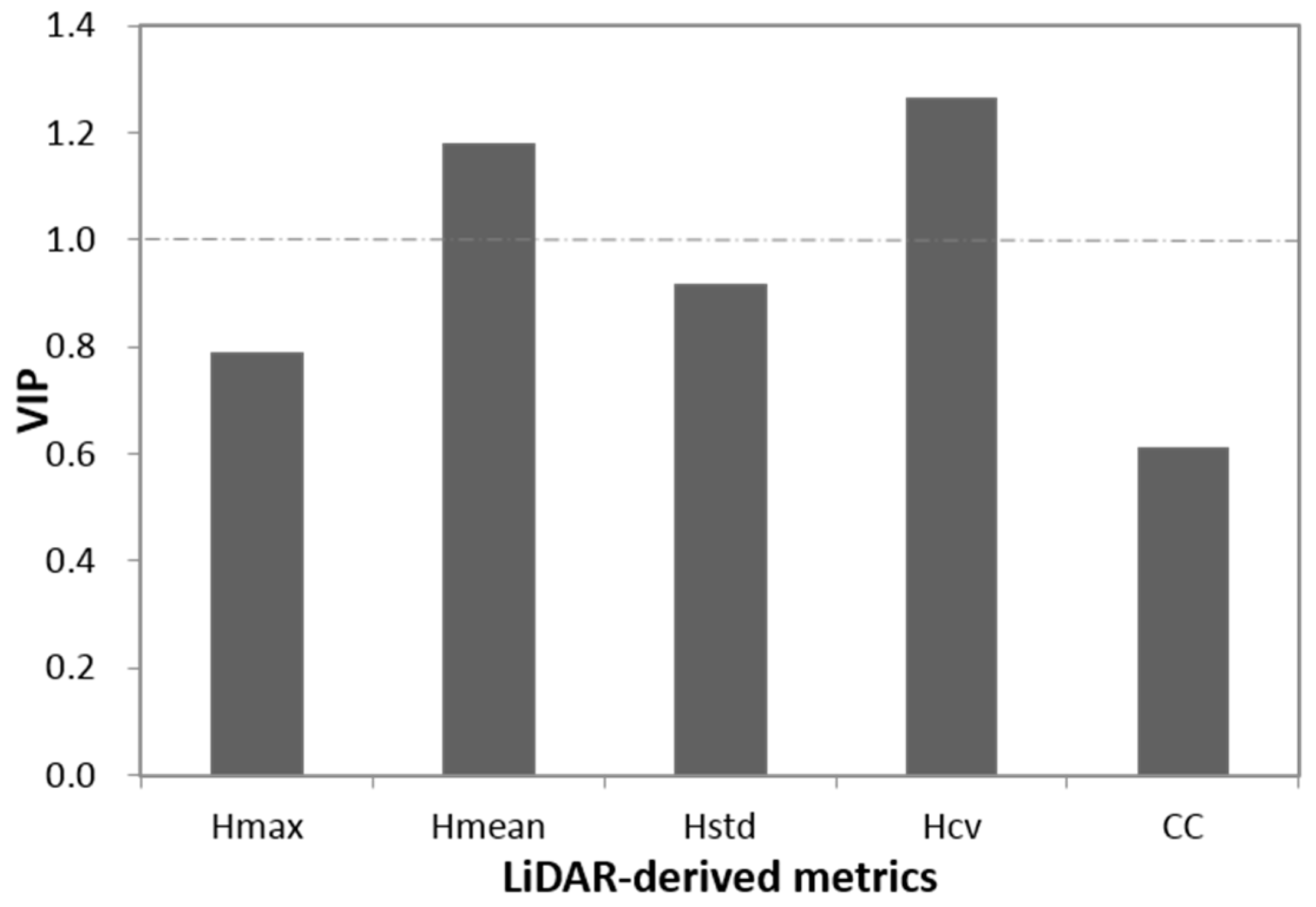
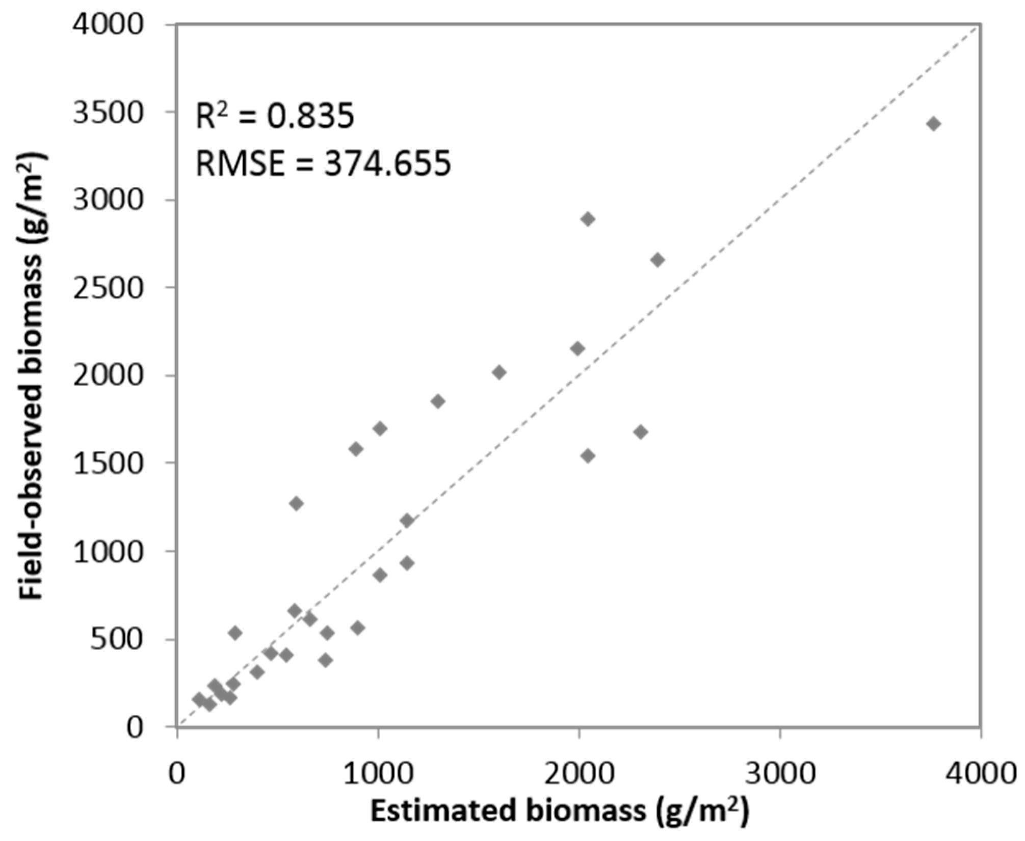
4.2. LiDAR-Derived Metrics as Predictors of Vegetation Biomass
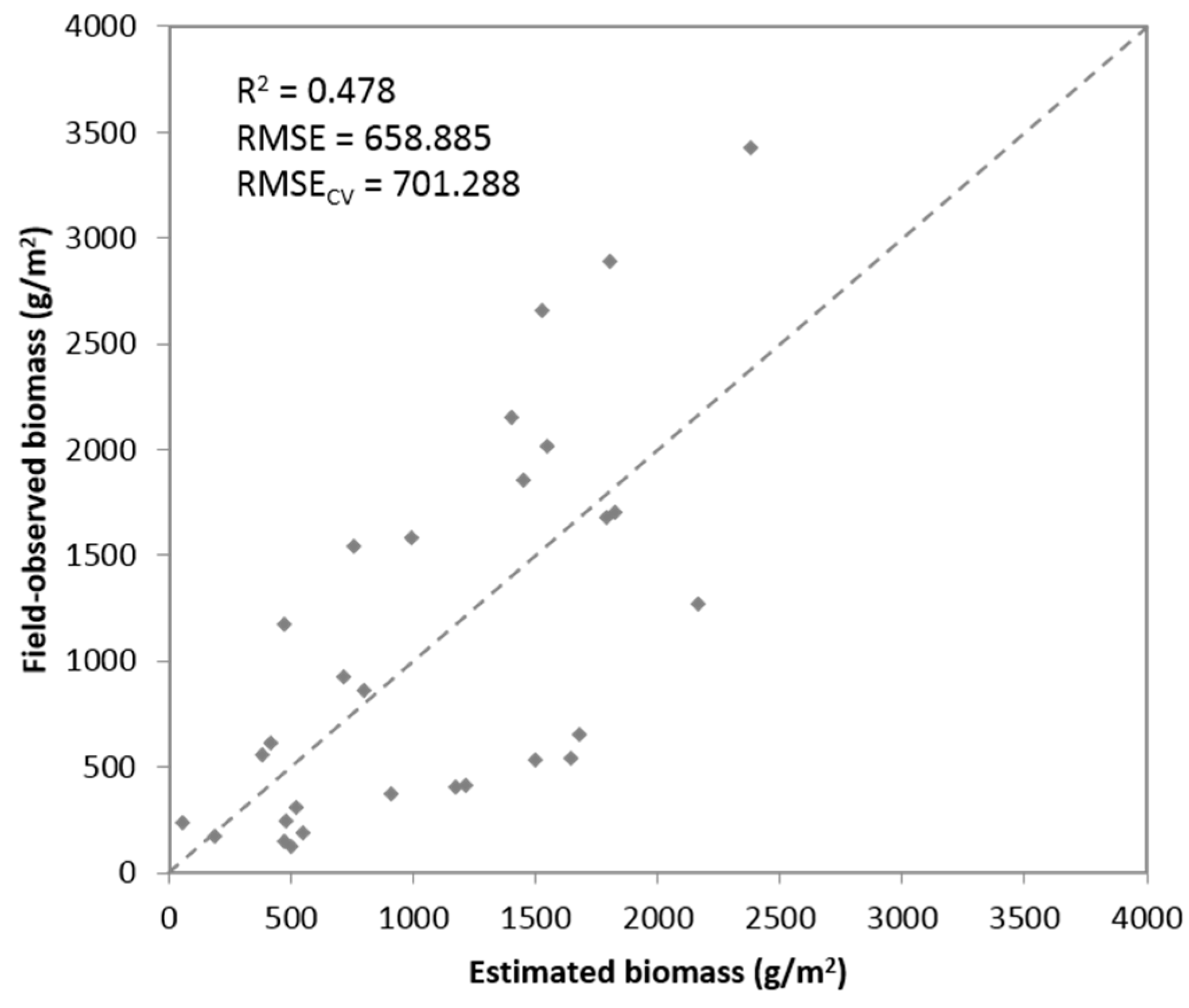
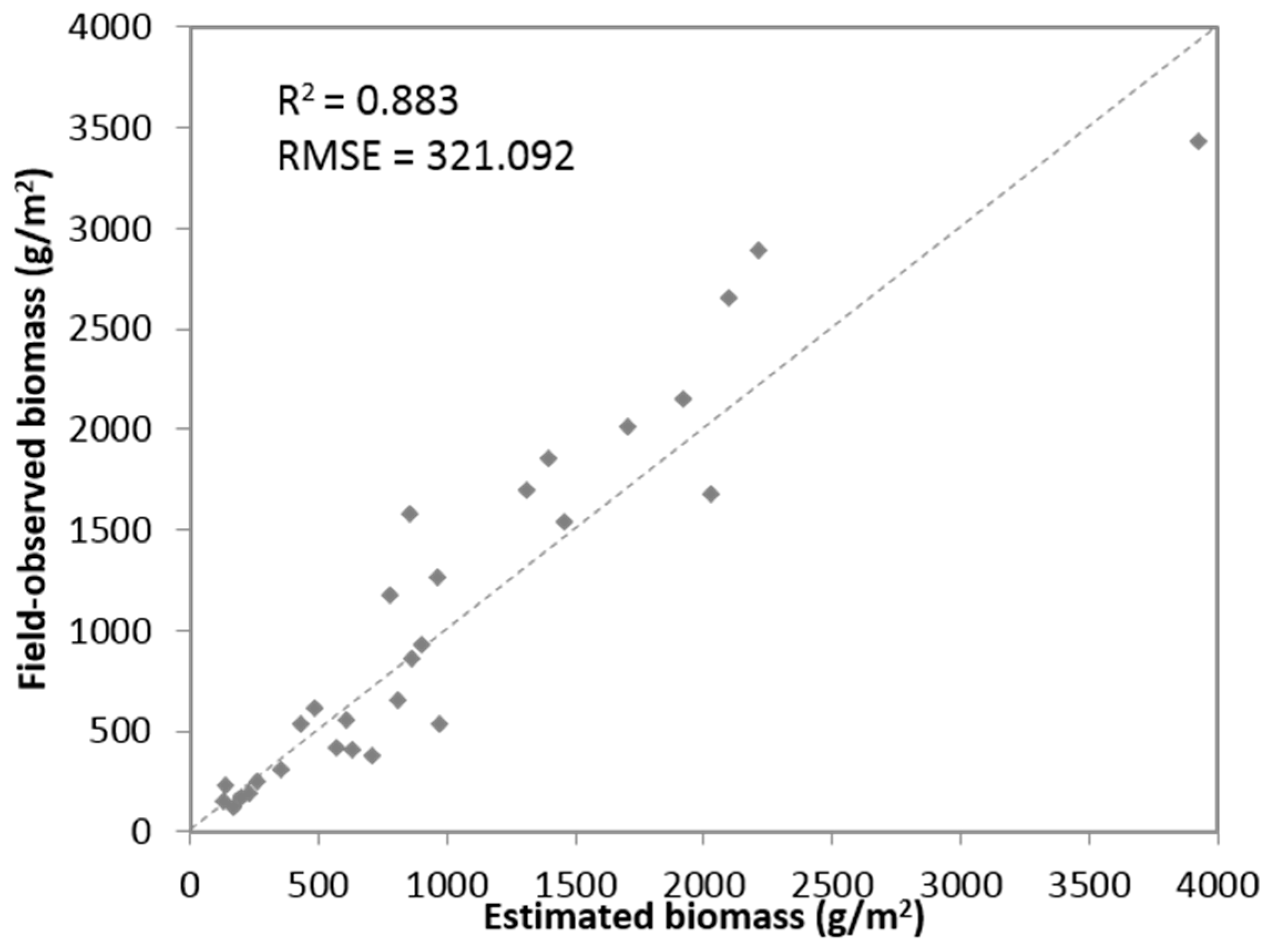
4.3. Fusion of LiDAR and Hyperspectral Data for Vegetation Biophysical Variables Predictions
5. Discussion
6. Conclusions
Acknowledgments
Author Contributions
Conflicts of Interest
References
- Gitelson, A.; Merzlyak, M.N. Spectral reflectance changes associated with autumn senescence of Aesculus hippocastanum L. and Acer platanoides L. Leaves. Spectral features and relation to chlorophyll estimation. J. Plant Physiol. 1994, 143, 286–292. [Google Scholar] [CrossRef]
- Liu, J.; Pattey, E.; Miller, J.R.; McNairn, H.; Smith, A.; Hu, B. Estimating crop stresses, aboveground dry biomass and yield of corn using multi-temporal optical data combined with a radiation use efficiency model. Remote Sens. Environ. 2010, 114, 1167–1177. [Google Scholar] [CrossRef]
- Chen, Q. Lidar remote sensing of vegetation biomass. Remote Sens. Nat. Resour. 2013, 399, 399–420. [Google Scholar]
- Pereira Coltri, P.; Zullo, J.; Ribeiro do Valle Goncalves, R.; Romani, L.A.S.; Pinto, H.S. Coffee crop’s biomass and carbon stock estimation with usage of high resolution satellites images. IEEE J. Sel. Top. Appl. Earth Obs. Remote Sens. 2013, 6, 1786–1795. [Google Scholar] [CrossRef]
- Eitel, J.U.H.; Magney, T.S.; Vierling, L.A.; Brown, T.T.; Huggins, D.R. Lidar based biomass and crop nitrogen estimates for rapid, non-destructive assessment of wheat nitrogen status. Field Crop. Res. 2014, 159, 21–32. [Google Scholar] [CrossRef]
- Li, W.; Niu, Z.; Huang, N.; Wang, C.; Gao, S.; Wu, C. Airborne lidar technique for estimating biomass components of maize: A case study in Zhangye City, Northwest China. Ecol Indic. 2015, 57, 486–496. [Google Scholar] [CrossRef]
- Haboudane, D.; Miller, J.R.; Pattey, E.; Zarco-Tejada, P.J.; Strachan, I.B. Hyperspectral vegetation indices and novel algorithms for predicting green LAI of crop canopies: Modeling and validation in the context of precision agriculture. Remote Sens. Environ. 2004, 90, 337–352. [Google Scholar] [CrossRef]
- Tilly, N.; Hoffmeister, D.; Cao, Q.; Huang, S.; Lenz-Wiedemann, V.; Miao, Y.; Bareth, G. Multitemporal crop surface models: Accurate plant height measurement and biomass estimation with terrestrial laser scanning in paddy rice. J. Appl. Remote Sens. 2014, 8. [Google Scholar] [CrossRef]
- Becker-Reshef, I.; Vermote, E.; Lindeman, M.; Justice, C. A generalized regression-based model for forecasting winter wheat yields in Kansas and Ukraine using MODIS data. Remote Sens. Environ. 2010, 114, 1312–1323. [Google Scholar] [CrossRef]
- Gao, S.; Niu, Z.; Huang, N.; Hou, X. Estimating the leaf area index, height and biomass of maize using HJ-1 and RADARSAT-2. Int. J. Appl. Earth Obs. Geoinf. 2013, 24, 1–8. [Google Scholar] [CrossRef]
- Jacquemoud, S.; Bacour, C.; Poilve, H.; Frangi, J.P. Comparison of four radiative transfer models to simulate plant canopies reflectance: Direct and inverse mode. Remote Sens. Environ. 2000, 74, 471–481. [Google Scholar] [CrossRef]
- Tang, S.; Chen, J.; Zhu, Q.; Li, X.; Chen, M.; Sun, R.; Zhou, Y.; Deng, F.; Xie, D. LAI inversion algorithm based on directional reflectance kernels. J. Environ. Manag. 2007, 85, 638–648. [Google Scholar] [CrossRef] [PubMed]
- Boegh, E.; Soegaard, H.; Broge, N.; Hasager, C.; Jensen, N.; Schelde, K.; Thomsen, A. Airborne multispectral data for quantifying leaf area index, nitrogen concentration, and photosynthetic efficiency in agriculture. Remote Sens. Environ. 2002, 81, 179–193. [Google Scholar] [CrossRef]
- Broge, N.H.; Mortensen, J.V. Deriving green crop area index and canopy chlorophyll density of winter wheat from spectral reflectance data. Remote Sens. Environ. 2002, 81, 45–57. [Google Scholar] [CrossRef]
- Wu, C.; Niu, Z.; Tang, Q.; Huang, W. Estimating chlorophyll content from hyperspectral vegetation indices: Modeling and validation. Agric. For. Meteorol. 2008, 148, 1230–1241. [Google Scholar] [CrossRef]
- Nguy-Robertson, A.L.; Peng, Y.; Gitelson, A.A.; Arkebauer, T.J.; Pimstein, A.; Herrmann, I.; Karnieli, A.; Rundquist, D.C.; Bonfil, D.J. Estimating green LAI in four crops: Potential of determining optimal spectral bands for a universal algorithm. Agric. For. Meteorol. 2014, 192–193, 140–148. [Google Scholar] [CrossRef]
- Xie, Q.; Huang, W.; Liang, D.; Chen, P.; Wu, C.; Yang, G.; Zhang, J.; Huang, L.; Zhang, D. Leaf area index estimation using vegetation indices derived from airborne hyperspectral images in winter wheat. IEEE J. Sel. Top. Appl. Earth Obs. Remote Sens. 2014, 7, 3586–3594. [Google Scholar] [CrossRef]
- Gong, P.; Pu, R.; Biging, G.S.; Larrieu, M.R. Estimation of forest leaf area index using vegetation indices derived from hyperion hyperspectral data. IEEE Trans. Geosci. Remote Sens. 2003, 41, 1355–1362. [Google Scholar] [CrossRef]
- Koetz, B.; Sun, G.; Morsdorf, F.; Ranson, K.J.; Kneubuehler, M.; Itten, K.; Allgoewer, B. Fusion of imaging spectrometer and lidar data over combined radiative transfer models for forest canopy characterization. Remote Sens. Environ. 2007, 106, 449–459. [Google Scholar] [CrossRef]
- Gilmore, M.S.; Wilson, E.H.; Barrett, N.; Civco, D.L.; Prisloe, S.; Hurd, J.D.; Chadwick, C. Integrating multi-temporal spectral and structural information to map wetland vegetation in a lower connecticut river tidal marsh. Remote Sens. Environ. 2008, 112, 4048–4060. [Google Scholar] [CrossRef]
- Delegido, J.; Alonso, L.; González, G.; Moreno, J. Estimating chlorophyll content of crops from hyperspectral data using a normalized area over reflectance curve (NAOC). Int. J. Appl. Earth Obs. Geoinf. 2010, 12, 165–174. [Google Scholar] [CrossRef]
- Hladik, C.; Schalles, J.; Alber, M. Salt marsh elevation and habitat mapping using hyperspectral and LiDAR data. Remote Sens. Environ. 2013, 139, 318–330. [Google Scholar] [CrossRef]
- Zhao, K.; Valle, D.; Popescu, S.; Zhang, X.; Mallick, B. Hyperspectral remote sensing of plant biochemistry using bayesian model averaging with variable and band selection. Remote Sens. Environ. 2013, 132, 102–119. [Google Scholar] [CrossRef]
- Chen, J.M.; Cihlar, J. Retrieving leaf area index of boreal conifer forests using Landsat TM images. Remote Sens. Environ. 1996, 55, 153–162. [Google Scholar] [CrossRef]
- Vaglio Laurin, G.; Chen, Q.; Lindsell, J.A.; Coomes, D.A.; Frate, F.D.; Guerriero, L.; Pirotti, F.; Valentini, R. Above ground biomass estimation in an African tropical forest with LiDAR and hyperspectral data. ISPRS J. Photogramm. 2014, 89, 49–58. [Google Scholar] [CrossRef]
- Cui, Y.; Zhao, K.; Fan, W.; Xu, X. Retrieving crop fractional cover and LAI based on airborne LiDAR data. J. Remote Sens. 2011, 15, 1276–1288. [Google Scholar]
- Hofle, B. Radiometric correction of terrestrial LiDAR point cloud data for individual maize plant detection. IEEE Geosci. Remote Sens. Lett. 2014, 11, 94–98. [Google Scholar] [CrossRef]
- Zhao, K.; Popescu, S.; Nelson, R. LiDAR remote sensing of forest biomass: A scale-invariant estimation approach using airborne lasers. Remote Sens. Environ. 2009, 113, 182–196. [Google Scholar] [CrossRef]
- Clark, M.L.; Roberts, D.A.; Ewel, J.J.; Clark, D.B. Estimation of tropical rain forest aboveground biomass with small-footprint LiDAR and hyperspectral sensors. Remote Sens. Environ. 2011, 115, 2931–2942. [Google Scholar] [CrossRef]
- Swatantran, A.; Dubayah, R.; Roberts, D.; Hofton, M.; Blair, J.B. Mapping biomass and stress in the Sierra Nevada using LiDAR and hyperspectral data fusion. Remote Sens. Environ. 2011, 115, 2917–2930. [Google Scholar] [CrossRef]
- Luo, S.; Wang, C.; Pan, F.; Xi, X.; Li, G.; Nie, S.; Xia, S. Estimation of wetland vegetation height and leaf area index using airborne laser scanning data. Ecol. Indic. 2015, 48, 550–559. [Google Scholar] [CrossRef]
- Nie, S.; Wang, C.; Dong, P.; Xi, X. Estimating leaf area index of maize using airborne full-waveform lidar data. Remote Sens. Lett. 2016, 7, 111–120. [Google Scholar] [CrossRef]
- Luo, S.; Wang, C.; Xi, X.; Pan, F. Estimating FPAR of maize canopy using airborne discrete-return lidar data. Opt. Express 2014, 22, 5106–5117. [Google Scholar] [CrossRef] [PubMed]
- Asner, G.P.; Knapp, D.E.; Kennedy-Bowdoin, T.; Jones, M.O.; Martin, R.E.; Boardman, J.; Field, C.B. Carnegie airborne observatory: In-flight fusion of hyperspectral imaging and waveform light detection and ranging for three-dimensional studies of ecosystems. J. Appl. Remote Sens. 2007, 1. [Google Scholar] [CrossRef]
- Anderson, J.; Plourde, L.; Martin, M.; Braswell, B.; Smith, M.; Dubayah, R.; Hofton, M.; Blair, J. Integrating waveform LiDAR with hyperspectral imagery for inventory of a northern temperate forest. Remote Sens. Environ. 2008, 112, 1856–1870. [Google Scholar] [CrossRef]
- Latifi, H.; Fassnacht, F.; Koch, B. Forest structure modeling with combined airborne hyperspectral and LiDAR data. Remote Sens. Environ. 2012, 121, 10–25. [Google Scholar] [CrossRef]
- Kulawardhana, R.W.; Popescu, S.C.; Feagin, R.A. Fusion of LiDAR and multispectral data to quantify salt marsh carbon stocks. Remote Sens. Environ. 2014, 154, 345–357. [Google Scholar] [CrossRef]
- Lin, X.; Zhang, J. Segmentation-based filtering of airborne LiDAR point clouds by progressive densification of terrain segments. Remote Sens. 2014, 6, 1294–1326. [Google Scholar] [CrossRef]
- Axelsson, P. DEM generation from laser scanner data using adaptive tin models. Int. Arch. Photogramm. Remote Sens. 2000, 33, 111–118. [Google Scholar]
- Li, X.; Cheng, G.; Liu, S.; Xiao, Q.; Ma, M.; Jin, R.; Che, T.; Liu, Q.; Wang, W.; Qi, Y. Heihe watershed allied telemetry experimental research (HiWATER): Scientific objectives and experimental design. Bull. Am. Meteorol. Soc. 2013, 94, 1145–1160. [Google Scholar] [CrossRef]
- Matthew, M.W.; Adler-Golden, S.M.; Berk, A.; Felde, G.; Anderson, G.P.; Gorodetzky, D.; Paswaters, S.; Shippert, M. Atmospheric correction of spectral imagery: Evaluation of the flaash algorithm with AVIRIS data. In Proceedings of the IEEE Applied Imagery Pattern Recognition Workshop, Washington, DC, USA, 16–18 October 2002; pp. 157–163.
- Berk, A.; Bernstein, L.; Anderson, G.; Acharya, P.; Robertson, D.; Chetwynd, J.; Adler-Golden, S. Modtran cloud and multiple scattering upgrades with application to AVIRIS. Remote Sens. Environ. 1998, 65, 367–375. [Google Scholar] [CrossRef]
- Thomas, V.; Finch, D.A.; McCaughey, J.H.; Noland, T.; Rich, L.; Treitz, P. Spatial modelling of the fraction of photosynthetically active radiation absorbed by a boreal mixedwood forest using a LiDAR-hyperspectral approach. Agric. For. Meteorol. 2006, 140, 287–307. [Google Scholar] [CrossRef]
- Jordan, C.F. Derivation of leaf-area index from quality of light on the forest floor. Ecology 1969, 50, 663–666. [Google Scholar] [CrossRef]
- Rouse, J., Jr. Monitoring the Vernal Advancement and Retrogradation (Green Wave Effect) of Natural Vegetation; NASA Technical Reports Server: Hampton, VA, USA, 1974.
- Qi, J.; Chehbouni, A.; Huete, A.; Kerr, Y.; Sorooshian, S. A modified soil adjusted vegetation index. Remote Sens. Environ. 1994, 48, 119–126. [Google Scholar] [CrossRef]
- Gitelson, A.A.; Viña, A.; Arkebauer, T.J.; Rundquist, D.C.; Keydan, G.; Leavitt, B. Remote estimation of leaf area index and green leaf biomass in maize canopies. Geophys. Res. Lett. 2003, 30. [Google Scholar] [CrossRef]
- Jin, X.; Yang, G.; Xu, X.; Yang, H.; Feng, H.; Li, Z.; Shen, J.; Lan, Y.; Zhao, C. Combined multi-temporal optical and radar parameters for estimating LAI and biomass in winter wheat using HJ and RADARSAR-2 data. Remote Sens. 2015, 7, 13251–13272. [Google Scholar] [CrossRef]
- Luo, S.; Wang, C.; Xi, X.; Pan, F.; Peng, D.; Zou, J.; Nie, S.; Qin, H. Fusion of airborne LiDAR data and hyperspectral imagery for aboveground and belowground forest biomass estimation. Ecol. Indic. 2017, 73, 378–387. [Google Scholar] [CrossRef]
- Brovelli, M.A.; Crespi, M.; Fratarcangeli, F.; Giannone, F.; Realini, E. Accuracy assessment of high resolution satellite imagery orientation by leave-one-out method. ISPRS J. Photogramm. Remote Sens. 2008, 63, 427–440. [Google Scholar] [CrossRef]
- Peduzzi, A.; Wynne, R.H.; Thomas, V.A.; Nelson, R.F.; Reis, J.J.; Sanford, M. Combined use of airborne LiDAR and DBinSAR data to estimate LAI in temperate mixed forests. Remote Sens. 2012, 4, 1758–1780. [Google Scholar] [CrossRef]


| Min | Max | Mean | SD | |
| Height (cm) | 121.82 | 309.09 | 228.62 | 0.52 |
| LAI | 1.59 | 4.69 | 2.88 | 0.9 |
| Biomass (g/m2) | 126.12 | 3428.78 | 1078.61 | 912.08 |
| Index | Abbr. | Formula |
|---|---|---|
| Simple Ratio Vegetation Index | ||
| Normalized Difference Vegetation Index | ||
| Modified Simple Ratio Index | ||
| Modified Soil-Adjusted Vegetation Index | ||
| Red Edge NDVI | ||
| Red Edge Modified Simple Ratio Index |
| Index | Abbr. | Formula |
|---|---|---|
| Max height | , | |
| Mean height | ||
| Standard deviation | ||
| Coefficient of variation | ||
| Canopy cover |
| VIs | SR | NDVI | MSR | MSAVI | ReNDVI | ReMSR |
| SR | 1.000 | 0.986 | 0.893 | 0.996 | 0.896 | 0.900 |
| NDVI | 0.986 | 1.000 | 0.953 | 0.996 | 0.951 | 0.959 |
| MSR | 0.893 | 0.953 | 1.000 | 0.927 | 0.969 | 0.995 |
| MSAVI | 0.996 | 0.996 | 0.927 | 1.000 | 0.925 | 0.933 |
| ReNDVI | 0.896 | 0.951 | 0.969 | 0.925 | 1.000 | 0.989 |
| ReMSR | 0.900 | 0.959 | 0.995 | 0.933 | 0.989 | 1.000 |
© 2016 by the authors; licensee MDPI, Basel, Switzerland. This article is an open access article distributed under the terms and conditions of the Creative Commons Attribution (CC-BY) license (http://creativecommons.org/licenses/by/4.0/).
Share and Cite
Wang, C.; Nie, S.; Xi, X.; Luo, S.; Sun, X. Estimating the Biomass of Maize with Hyperspectral and LiDAR Data. Remote Sens. 2017, 9, 11. https://doi.org/10.3390/rs9010011
Wang C, Nie S, Xi X, Luo S, Sun X. Estimating the Biomass of Maize with Hyperspectral and LiDAR Data. Remote Sensing. 2017; 9(1):11. https://doi.org/10.3390/rs9010011
Chicago/Turabian StyleWang, Cheng, Sheng Nie, Xiaohuan Xi, Shezhou Luo, and Xiaofeng Sun. 2017. "Estimating the Biomass of Maize with Hyperspectral and LiDAR Data" Remote Sensing 9, no. 1: 11. https://doi.org/10.3390/rs9010011
APA StyleWang, C., Nie, S., Xi, X., Luo, S., & Sun, X. (2017). Estimating the Biomass of Maize with Hyperspectral and LiDAR Data. Remote Sensing, 9(1), 11. https://doi.org/10.3390/rs9010011