1. Introduction
Terrestrial snow cover and glaciers are major components of the cryosphere, representing two of the fastest-changing geographical features on the earth’s surface. They occur over a large proportion of the Earth’s continents. They are also sensitive indicators of climate change because they show a wide range of responses to variations in global temperature. Snow cover extent in the Northern Hemisphere is greatest in January of each year, encompassing an average area of 46.5 million·km
2. The annual average areal cover is approximately 25.3 million·km
2, with a standard deviation of 1.1 million·km
2 [
1]. In arid regions such as the Tarim River Basin in China, mountain-fed rivers are the only available water sources that can meet societal needs such as public supply, agriculture, irrigation, and hydropower. Hence, variation in the extent of snow cover in the Tarim Basin might affect subsequent spring and summer river runoff, which could have an impact on the socioeconomic development of the region, disturb fragile ecosystems, and even lead to an increase in the frequency of droughts and/or flood-related disasters [
2]. The mapping of snow cover is important for both the calculation of energy balances and the prediction of climate patterns; therefore, its accurate determination is of paramount importance [
3].
Recent technological advances in remote sensing have made it possible to use satellite data to extract historical and near real-time information on the areal amount and extent of snow cover. Of the many options available, the Snow Cover Daily L3 Global 500-m Grid (MOD10A1) dataset is used widely to monitor daily changes in the spatiotemporal distribution of snow over large areas. This freely available global dataset, which has undergone many reprocessing steps, has proven highly useful for the monitoring and mapping of snow cover changes at high temporal frequency [
4,
5,
6].
One MODIS (MODerate-resolution Imaging Spectroradiometer) scan line is composed of 2708 observations at 500-m intervals, where the sensor zenith angle (SZA) approaches 65° at the end of each profile [
7]. Pixels representing snow cover in MOD10A1 are selected by a scoring algorithm that uses observations obtained nearest to local noon and closest to the SZA nadir [
8]. However, the large cross-track scan angle of MODIS has raised doubts about the quality of MOD10A1 data at the end of each scan line. Uncertainty related to the estimation of snow cover at high values of SZA is mentioned in the MOD10A1 official documentation [
9], which has led many workers to investigate the effect of viewing geometry on the image reflectance, normalized index, and pixel areas [
10]. Associated studies have also been conducted into the influence of topography or underlying surface conditions [
11].
Variations in the SZA and solar zenith angle in relation to the canopy reflectance of wheat have shown that the ratio of off-nadir to nadir radiance increases (or decreases) as SZA increases (or decreases) [
12]. MODIS Level-3 data have also been used to quantify the effects of SZA on the cloud properties of MODIS, which revealed that the amount of cloud “observed” by MODIS increases remarkably between the nadir and the scan-line terminus [
13]. A lower SZA was found to coincide with higher reflectance, and vice versa [
14], which led to the discovery of inaccuracies in snow cover pixels at off-nadir viewing angles. The primary source of error in this case is thought to stem from pixel expansion at off-nadir viewing angles, which leads to neighboring (non-snow-covered) pixels adopting incorrect reflectance values [
15]. A semiempirical parametric model of the angular pattern of snow cover in forested areas has been established [
16]. Errors in snow cover estimation are exacerbated for large SZAs in forested areas [
17] because the snow-covered canopy causes the sensor to interpret a greater snow cover fraction at near-nadir views. By contrast, observable snow cover is reduced at the end of a MODIS scan line.
Some researchers have attempted to define suitable SZA thresholds that produce accurate pixel data from MODIS. Gridding artifacts have been found to affect the spatial properties of MODIS images because of mismatches between observed and predefined pixels when viewing zenith angles are high. In the along-track direction for 500-m data, the overlap between consecutive scan lines is larger than the observation’s dimensions when the viewing zenith angle is ~27° [
18]. The angular threshold for the MODIS Snow Cover Area (SCA) and Grain Size (MODSCAG) snow cover model was determined to be 25°, with a deviation of up to 10%, calculated from the area at nadir for the MODIS pixels considered [
19,
20].
These studies have demonstrated that the variation in the SZA is intimately linked with uncertainty in the radiance or reflectance of MODIS data, which could ultimately result in the incorrect identification of targets such as wheat, cloud, vegetation, and/or snow cover. Pixel expansion and a “gridding” effect have been proposed as causes for this inaccuracy, and a preliminary linear relationship has been found between SZA and reflectance values. However, there is no firm conclusion or consensus about the value of the optimal SZA threshold, or how the SZA influences the final MODIS product. Determination of an angular threshold for MODSCAG requires investigation of the influence of SZA on MOD10A1 data. This work focused on investigating the relationship between the SCA of MOD10A1 data and its corresponding SZA in the Tarim River Basin, in order to produce daily snow cover data with greater reliability. A paired-date difference method was used for comparative analysis, which allowed the mechanism of overestimation to be determined based on statistical data obtained from five subwatersheds over a 10-year period. After determining an optimal threshold for a reliable SZA, a multiday refilling method was used to replace pixels related to large SZA values and high cloud cover with new snow cover interpretations. This modified dataset was evaluated in terms of its monthly and annual averages of snow cover percentage (SCP) and snow cover frequency (SCF), and it was validated using 30-m-resolution HJ-1A/B satellite data. The results indicated that the modified snow cover dataset presented herein is significantly more accurate than the unmodified version currently available.
2. Study Area and Data
2.1. Study Area
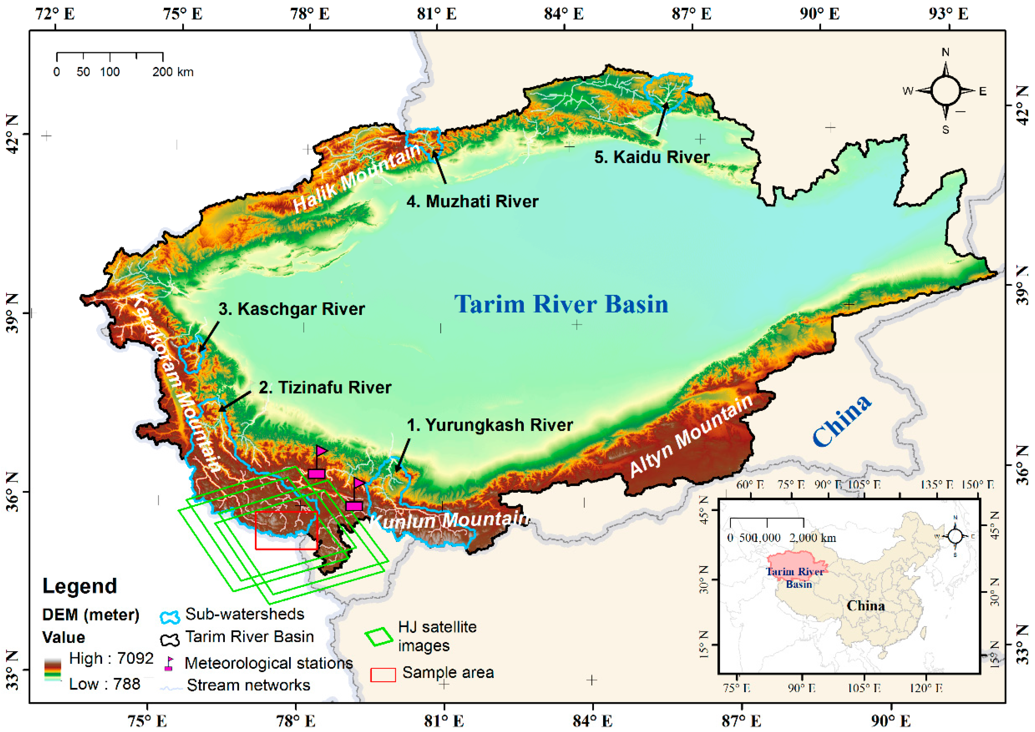
The Tarim River Basin is the largest continental river basin in China. It is bordered by the Qinghai–Tibetan Plateau and the Tianshan, Kunlun, and Altyn Mountain Ranges (
Figure 1). These mountains act as a block to the inward passage of warm and moist air, which has caused the Tarim River Basin to develop an extremely dry, desert microclimate with limited precipitation and high potential evaporation [
21,
22]. Annual precipitation in the mountainous headwater regions can reach ~250 mm, as opposed to 40–70 mm in the downstream regions of the basin. The Taklamakan Desert and the Lop Nur Basin have average annual precipitation of ~12 mm and annual potential evaporation of ~1000–1600 mm; thus, the Tarim River Basin has the highest aridity index in the world [
23]. Most snow cover—a key source of fresh water—occurs over the high-elevation parts of the basin, such as the western Tianshan area in the northwest, Pamirs and Karakorum Mountains in the west, Kunlun Mountains in the south, and Tianshan Mountains in the northeast. This limited and unevenly distributed resource makes the Tarim River Basin an ecologically vulnerable environment, which exemplifies the need for improved resource management and climatic and environmental governance.
2.2. Data Description
The MOD10A1 and MOD09GA (Surface Reflectance Daily L2G Global 500 m) datasets were used to determine the influence of SZA on snow cover and to calculate the daily SCA in the Tarim River Basin from 1 October 2002, to 30 September 2012 [
24,
25]. MOD10A1 data are based on a snow-cover-mapping algorithm that relies mainly on the normalized difference snow index (NDSI). Snow maps have been produced automatically on a daily basis at the National Snow and Ice Data Center Distributed Active Archive Center of the National Aeronautics and Space Administration (NASA) since 1999. This dataset has 500-m spatial resolution and it is gridded to a sinusoidal map projection of 7600 tiles of MOD10A1 data, which are compressed to a Hierarchical Data Format–Earth Observing System format [
8]. For this study, tiles h24v4, h25v4, h24v5, and h25v5 that covered the entire Tarim River Basin area were downloaded.
SZA data and reflectance data obtained from the MOD09GA dataset were downloaded from NASA’s Earth Observing System Data and Information System’s ECHO using the Reverb client. The MOD09GA provides seven bands of 500-m resolution daily surface reflectance data, and 1-km resolution observation and geolocation statistics. The latter low-resolution datasets were used to obtain the SZA degree data, which were represented as 16-bit signed integers to denote the SZA values in each tile [
26].
Meteorological data were downloaded from the National Meteorological Information Center of China website (
http://data.cma.cn/). Here, we used the dataset titled “Chinese terrestrial climate data,” which contains daily meteorological data obtained at ground stations since 1951. Relevant records for our study comprised daily precipitation (including snow depth information), and daily average, maximum, and minimum temperatures. Most meteorological stations in the Tarim River Basin are located in its snow-free interior, although some are peripheral to the snow-covered areas. As such, the small amount of meteorological data collected at the periphery of the basin cannot effectively assist in identifying the degree to which MOD10A1 data overestimate snow cover. Nonetheless, data for precipitation (snow) and temperature recorded by those stations closest to our study area (i.e., Tashkurghan and Pishan) were used as auxiliary data to understand the effects of snowfall within the region.
The Huanjing (HJ) satellite constellation was launched by the Chinese government on 6 September 2008, to monitor disasters and environmental conditions. The multitemporal, multispectral charge-coupled device (CCD) data and infrared scanner (IRS) data collected by HJ-1A and HJ-1B (two optical satellites with 30-m spatial resolution) were used as references to validate the MOD10A1 snow cover data (green boxes in
Figure 1). In theory, the four-day return period of each optical satellite could be used to provide daily, continuous CCD images by integrating two or more paths, which would validate the MOD10A1 snow cover data; however, the 30-m spatial resolution IRS data obtained by HJ-1A/B were also considered sufficient for validation purposes and were used as such herein. HJ-1A/B images acquired on 14–17 May 2011, were downloaded from the China Centre for Resources Satellite Data and Application website (
http://www.cresda.com), and their sensor types and path/row numbers are listed in
Table 1. The snow map method proposed by Dozier [
7,
8] was applied in our work in order to produce snow cover maps from the HJ-1A/B images. Sixty additional HJ-1A/B images were used to validate the modified product; their acquisition dates, orbit numbers, coordinates, and accuracies are listed in
Table S1.
3. Methodology
Snow-covered areas identified from MOD10A1 data were compared with reference data obtained from the HJ-1A/B satellite in the same area in order to verify the amount of overestimation of the former at large SZA values. Snow-melting periods (May–September) were selected for the study period, and data from the meteorological station were used to exclude those dates that registered snowfall events. For comparison purposes, suitable MOD10A1 data were also required for the same area and for dates consistent with the available HJ-1A/B satellite images. Visual inspection of the imagery resulted in the selection of four continuous days (14–17 May 2011) of cloud-free MOD10A1 data and HJ-1A/B satellite data. Precipitation and temperature data from nearby meteorological stations verified that snowfall did not occur during this period.
Snow pixels in MOD10A1 were extracted for the sample area to calculate the extent of the snow-covered areas. These same areas were categorized from the HJ-1A/B data using a snow-mapping algorithm, such that a pixel was classified as a snow-covered area when the NDSI value was >0.4 and the near-infrared reflectance (Band 4 of HJ-CCD) was >0.11 [
9]. The snow-mapping algorithm has been proven capable of extracting the snow-covered area from the HJ satellite data [
27,
28]. Thus, the SCA and the valid SCPs of the MOD10A1 and HJ-1A/B data were calculated, and the maximum, minimum, and average values of the corresponding SZA were determined for each pixel. A comparison between these values was used to confirm that the snow-covered areas were overestimated in a typical sample locality.
Five typical subwatersheds were also investigated to explore the effect of SZA across the entire study area. These subwatersheds were selected based on their different elevations, which allowed representative coverage of the Tarim River Basin’s snow-covered areas. Analysis of the overestimation effect caused by the SZA required selection of suitable precipitation-free paired dates, with an effective index (such as the valid SCP) also calculated for comparison. Specifically, the paired dates used to analyze the SZA overestimation effect in the Tarim River Basin were selected primarily based on the following two factors: whether they occurred during the melting season or within 10 years of each other. The daily SCPs of these dates were calculated by dividing the daily SCA by the study region’s overall area, and the values of the daily SCPs and their dates were plotted on 10 curves showing these paired dates over the course of 10 years. The ascending limb of each curve indicates an increase in SCA (i.e., new snowfall events), while the descending limb indicates a period of depletion. To exclude snowfall events, we only considered those dates that lay on the descending limb of the SCP curve, and we used two consistent days from each as a valid date pair. Finally, we used the valid SCP instead of the SCP in order to eliminate the influence of cloud cover. The valid SCP was calculated from the ratio of the mutual SCA to the mutual cloud-free area in the same region on both dates in each pair. Thus, the difference between the valid SCPs on each of these two days more accurately reflected the trend in snow cover variation. The difference between the valid SCP and that of the SZA for each date pair was plotted for each of the five subwatersheds to analyze the relationship between the variations in both SZA and SCP.
The mechanism by which SCA overestimation occurred for large values of SZA was analyzed by exploring the different responses of surface reflectance at Bands 4 and 6 and the change in the NDSI value when the SZA increased. Surface reflectance data for Bands 4 and 6 were extracted from the MOD09GA dataset to calculate the NDSI index. The minimum SZA value that introduces an overestimation in snow cover pixels (i.e., the sensitive SZA threshold) was determined by comparing these values to those of standard snow cover in the area when the SZA was at its nadir.
To reduce cloud obstruction and to complement missing MOD10A1 data in areas with a large SZA, we performed a spatiotemporal refilling of the entire dataset. In particular, we assigned a land cover class to the most recent cloudless observation (within a window of a few days) to a MOD10A1 data cell that had cloud cover, and assumed that land cover changes would not have been very drastic within this intervening period. This processing technique was defined as a multiday refilling method. Finally, the modified dataset of snow cover was validated using the standard snow cover classification results from the HJ-1A/B satellite.
4. Results
4.1. Quantifying the SZA Effect for Typical MOD10A1 Data
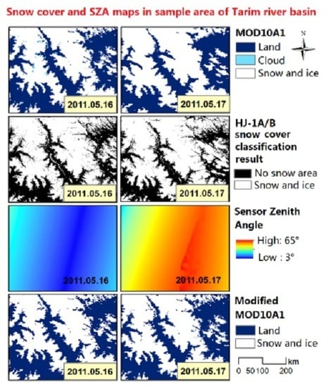
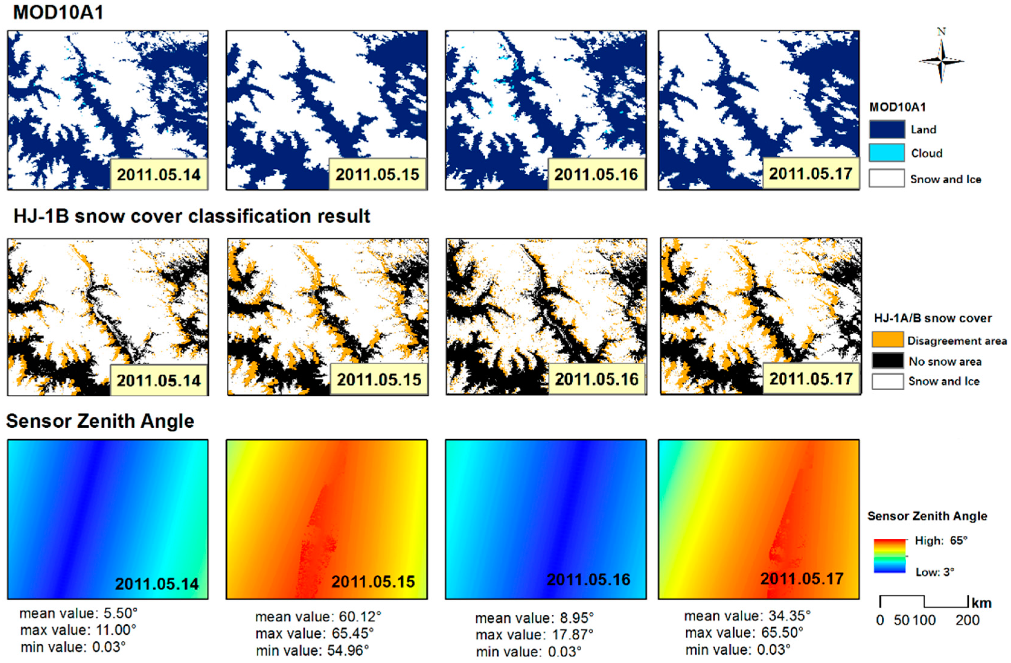
Figure 2 shows the snow cover distribution determined from the MOD10A1 and HJ-1A/B data, and their corresponding SZA distributions for four consecutive days in the study area within the Tarim River Basin (red box in
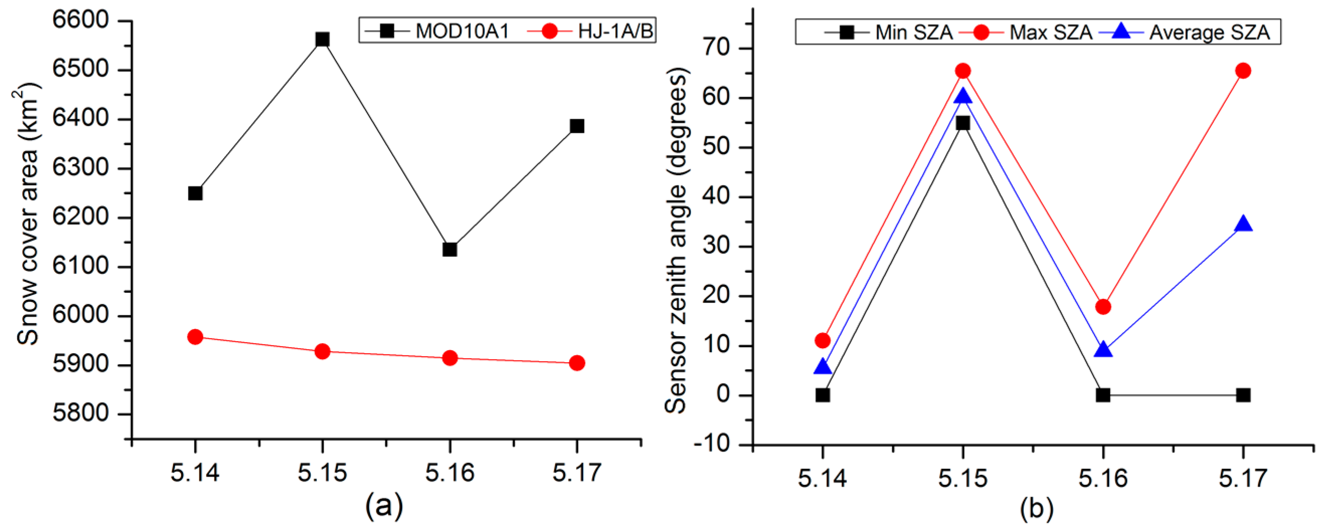
Figure 1). The corresponding SCAs for this four-day period are shown in
Figure 3a, and the maximum, minimum, and average SZA values are shown in
Figure 3b. A greater amount of detail on the snow cover information is missing from the MOD10A1 dataset on 15 and 17 May than that on 14 and 16 May (top row,
Figure 2). For example, the SCAs for 15 and 17 May are more expanded than those for 14 and 16 May because of the presence of a blurred margin for 15 and 17 May. As shown in the second row of
Figure 2, the disagreement area between HJ-1A/B and MOD10A are also larger for 15 and 17 May. The bottom row of
Figure 2 shows the corresponding SZA maps. It is evident that their values are elongated in a north–south direction each day, and that the absolute SZA values changed drastically each day. The SZA values on 15 and 17 May were higher than those on 14 and 16 May.
Figure 3a,b further verifies this areal contrast/overestimation phenomenon. The overall SCA of the sample area was ~8000 km
2. The reference SCA determined from the HJ-1A/B data changed slightly within this four-day period, having an average area of 5900 km
2. However, the SCA calculated from the MOD10A1 data during this period was not only higher than that derived from the HJ-1A/B data, but it also showed an oscillatory variation in amplitude by up to 200–300 km
2, accounting for 5% of the overall SCA. On 15 and 17 May, the average SZA values were clearly higher than those for the other two days; thus, the graphical and areal comparisons were successfully used to reveal this unusual expansion of the SCA during snow-melting periods, which was confirmed to be associated with an increase in SZA.
4.2. Analysis of SZA Effect in the Expanded Five Subwatersheds
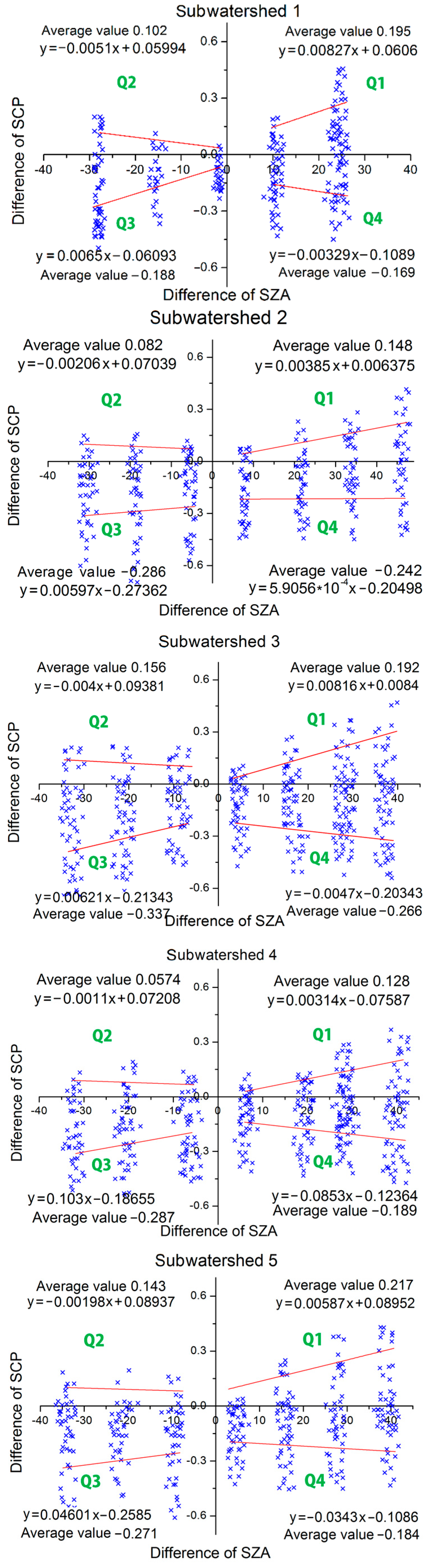
Based on the above result, we applied this technique to five subwatersheds of the Tarim River Basin during snow-melting periods using the same paired-date difference method (
Figure 4). In
Figure 4, the abscissa represents the SZA difference between the second day (15 August 2004) and the first day (14 August 2004), while the ordinate represents the valid SCP difference between the second and first days. Each scatter plot shows the change in the SCP difference based on the SZA difference for each of the subwatersheds over 10 hydrological years. Each scatter plot was divided similarly into four quadrants, where spots in the first quadrant represent suitable paired dates that showed an increase in both SZA and valid SCP from Day 1 to Day 2. A similar procedure was applied to the other quadrants.
Generally, there is no possibility of snow cover increasing during a snow-melting period. The valid SCP difference between the second and first days at such a time should therefore be negative, and data should plot at negative values on the ordinate. Reassuringly, most spots are distributed within the third and fourth quadrants in
Figure 4. However, even though these points indicate that snow cover decreased, the cause cannot be identified with confidence, as the reduction might have been the result of snow cover shrinkage during the depletion period or a decrease in the SZA value. Because it is difficult to distinguish the relative contribution of each mechanism, points plotted within these two quadrants were not analyzed further in this study. Nonetheless, some spots with positive ordinate values highlight an atypical increase in snow cover during the snow-melting period, but without new snowfall. Further investigation revealed more data points in the first quadrant than in the second quadrant, which showed that most of the increases in snow cover occurred when the SZA increased, verifying our initial hypothesis. Points in the second quadrant were interpreted as representing statistical errors or anomalies.
Average values and linear-fitting equations were calculated for valid SCP differences between the second and first days in each quadrant. We identified similarities in these data for all scatter plots, with the average first-quadrant values being consistently higher than second-quadrant values, indicating that the valid SCP increased more with increasing values of SZA. The absolute gradients of the fitting lines in the first quadrants were all larger than those in the second quadrants; indeed, the average values or gradients of the slopes for the first quadrant data were typically twice of those in the second quadrant. The linear relationship observed between the increases in valid SCP differences and SZA values in the first quadrant indicated that larger values of SZA lead to overestimation of SCP.
All the scatter plots contain groups of points that are aligned in columns at distinctly different distances along the abscissa. This is because of the change in the value of the SZA at the same location (i.e., the same pixel in the MOD10A1 data), which is related to the variation in the satellite’s orbital pattern. However, the SZA difference between two consecutive days was fixed, and therefore, the pixels in the same subwatershed were aligned by the same process that formulated the columns described above. The spatial areas of the different subwatersheds and the locations of areas where snowfall frequently occurred both affect the distance between these columns and their widths. Nonetheless, the point distributions observed still indicate a positive correlation between the SZA and SCP differences in all five subwatersheds. These experimental results, obtained from a large number of statistical data, adequately confirmed that a large value of SZA significantly affects the SCA estimation.
4.3. Analysis of the Mechanism Responsible for the SZA Effect
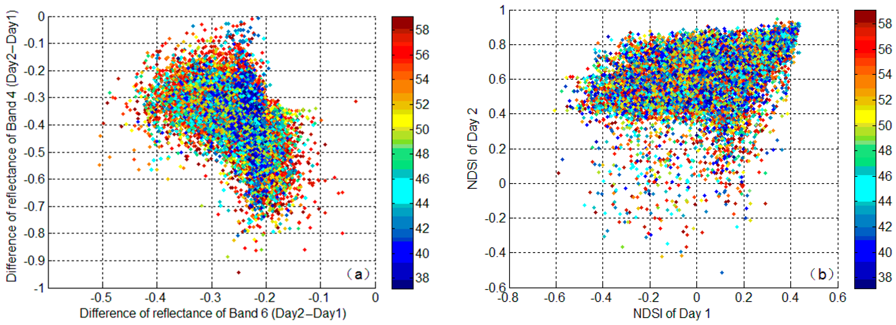
The mechanism responsible for the SZA effect was investigated using paired-date data points situated in the first quadrants of the aforementioned scatter plots. Data collected on 14 and 15 August 2004, during the snow-melting period, were chosen in this case. The SCA data for each day in same subwatershed were compared directly to calculate the amount of SCA on the second day. For each pixel of the overestimated area, the reflectance value differences between both days were plotted against the SZA differences for both days (
Figure 5).
Figure 5a shows that the Band-4 reflectance differences were negative, indicating that all such reflectance values decreased in the overestimated SCA following SZA increases. The average, maximum, and minimum values of the decreased reflectance were around −0.4, 0.0, and −0.95, respectively. The reflectance differences at Band 6 mainly ranged from −0.42 to −0.1, indicating that all such reflectances similarly decreased in the overestimated SCA when the SZA increased, although to a lesser degree. The average, maximum, and minimum values of the decreased reflectance at Band 6 were around −0.25, −0.05, and −0.51, respectively. Thus, the magnitude of decrease was larger for Band 4 than for Band 6.
Such unequal variation in reflectance between Bands 4 and 6 are interpreted as representing the spectral reflectance of snow being higher at green bands than at red bands, which has been corroborated by field-based experiments showing that different wavelengths produced different reflectances at different SZA values [
29]. The Algorithm Theoretical Basis Document for the MODIS Snow and Sea Ice-Mapping of a non-Lambertian reflector states that snow’s anisotropy might result in some errors when mapped at large view angles [
30]. The optical path through the atmosphere increases with higher values of SZA and shorter wavelengths, producing a larger bias in the Lambert reflectance [
31].
The different magnitudes of change at Bands 4 and 6 revealed an increased NDSI value in each pixel.
Figure 5b shows that the NDSI value on the first day was mainly between −0.6 and 0.4, whereas on the second day, it was mainly between 0.4 and 0.8. It is known that the NDSI value is critical for SCA identification using MOD10A1 data because the algorithm defines snow-covered pixels as those with an NDSI value of >0.4. Such an NDSI increase on the second day erroneously labeled pixels as snow covered, when in reality, this could not be the case in an area where no previous snowfall had been documented on the previous day during the snow-melting period. We therefore concluded that the main reason for SCA overestimation was a false increase in NDSI values caused by the different responses of Bands 4 and 6 to MODIS data when the SZA increased.
4.4. Determination of the Overestimation Threshold
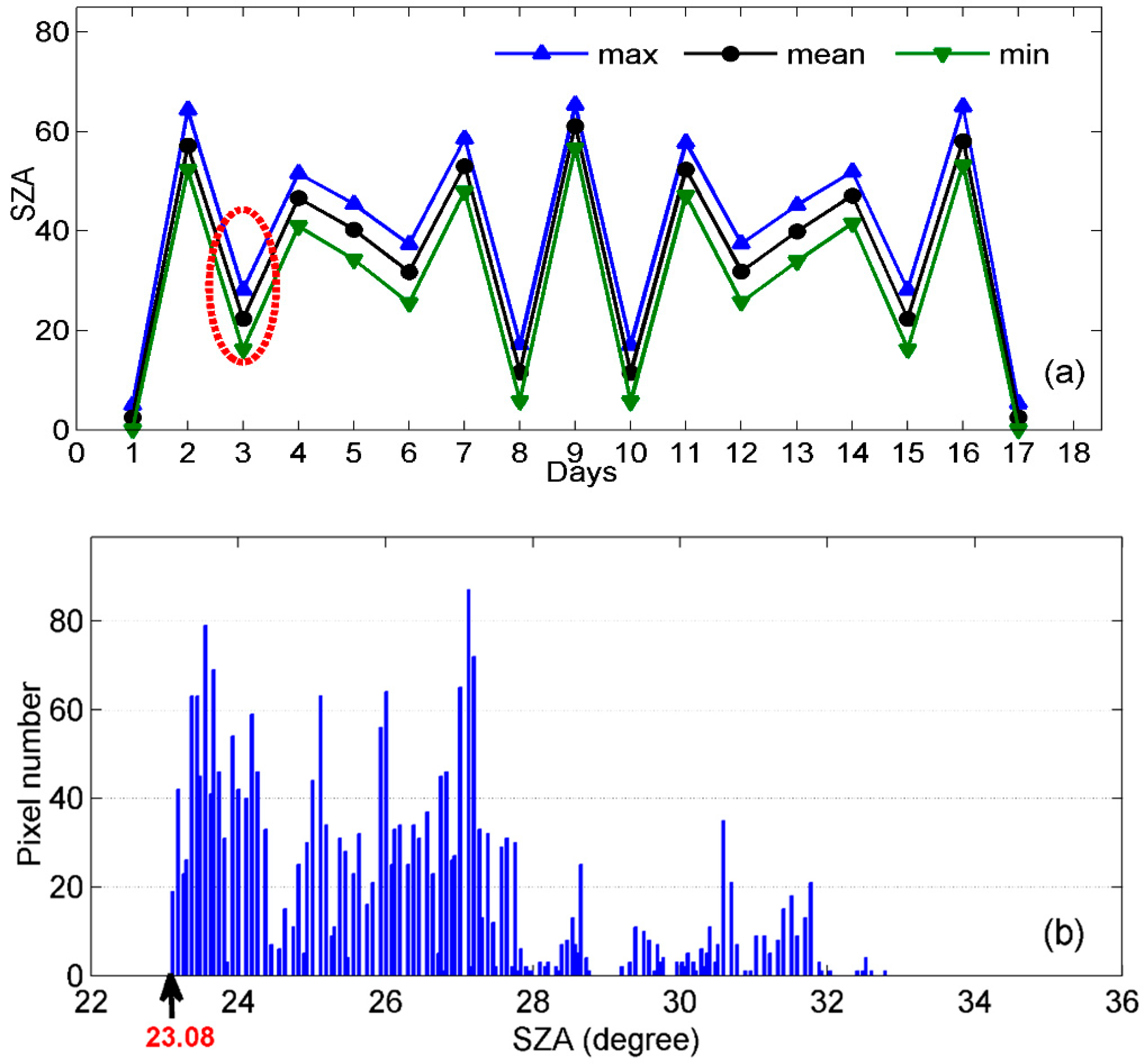
The positive correlation between overestimated SCA and increased SZA described above occurs extensively within the Tarim River Basin. From our results, it can be assumed that the erroneous expansion of snow-covered pixels would occur at a certain threshold value of SZA along a scan line between its nadir and its terminus. Snow pixel data obtained at SZA values larger than this threshold might therefore be untrustworthy. To delimit this threshold, we extracted data from a region within the Tarim River Basin with a nadir SZA (0° to 5°), and marked the imagery from that date as having been taken on “Day 1”. Owing to the 16-day cyclicity in SZA from MOD10A1, the following 16 days were also examined for comparative purposes. The highest, lowest, and average SZA values were calculated over this 17-day period (
Figure 6a) by averaging values obtained from 20 different test periods in the same region. We found that the SZA fluctuated for 16 days, and then returned to its original minimum value on the 17th day. Such a distinctive pattern existed across the entire Tarim River Basin.
Because of this cyclicity, we treated the SCA on Day 1 (SZA of 0° to 5°) as a benchmark that did not contain unwanted effects attributable to SZA; thus, all snow-covered areas determined during the following 16-day period would inevitably be considered influenced by the SZA effect. In theory, any minimum SZA value recorded during this 16-day period during snow melting that produced an SCA greater than that on the first day could be considered a possible threshold; therefore, in this work, we selected the third day for comparison with the first. This was done because the SZA value on the second day was nearly 60°, which was too high to determine a sensitive angular threshold. The third day had an appropriately low SZA value of between 16° and 30°, and it constituted only a short period from the first day. All other days were dismissed because of extensive shrinkage of the snowpack.
In order to find the lowest SZA that induced an overestimation, all pixels with emerging snow cover on the third day were recorded and plotted on a histogram with their corresponding SZA value (
Figure 6b). Over 750,000 pixels were collected for one test period, which produced a minimum SZA value of 23.08° for the emergence of new snow cover. This statistical test was conducted for 20 test periods and the calculated SZA minimum values ranged from 21.08° to 23.26°. We calculated a final optimal threshold of 22.37°, which represents the average of all 20 calculated minima, and we used this value to apply modifications to the snow cover data within the Tarim River Basin.
4.5. MOD10A1 Dataset Modification and Evaluation
We used the optimal threshold described above to modify the MOD10A1 snow cover data for the Tarim River Basin as follows. Firstly, we resampled the SZA images onto a 500-m-resolution grid for consistency, and then overlaid the MOD10A1 and SZA data and marked all pixels in MOD10A1 with SZA ≥22.37° as the missing data. Finally, a multiday refilling method [
32] was used to replace the missing data, so as to produce a modified snow cover dataset free of cloud and the SZA effect.
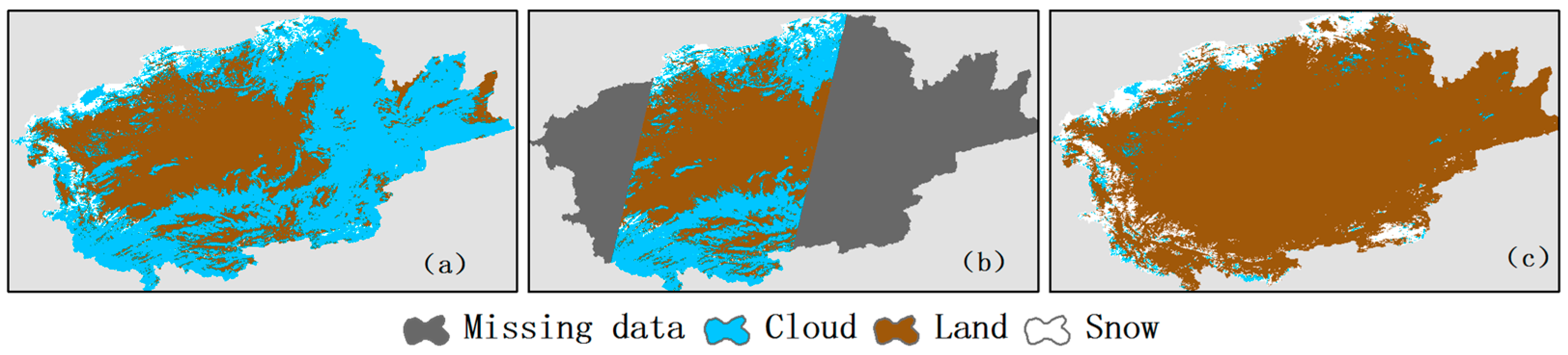
Figure 7 shows a comparison of maps produced before and after the modification of the snow cover data in the Tarim River Basin on 18 November 2003.
Figure 7a shows the original map derived from the MOD10A1 data,
Figure 7b shows the map from
Figure 7a after the removal of pixels with an SZA value ≥22.37° threshold (missing data are colored gray), and
Figure 7c shows the modified snow cover map after applying the cloud-removal method to the map shown in
Figure 7b.
Figure 7a shows that there was an extensive cloud cover (blue) across the entire research area and that visible snow-covered areas were indistinguishable. Additionally,
Figure 7b shows that almost half the area of study of the Tarim River Basin would have been influenced detrimentally by the effect of the large SZA (gray-colored areas). The SCA MOD10A1 data that fall within the SZA limits of confidence are therefore quite limited. The modified map (
Figure 7c) illustrates that the snow-covered areas can be identified clearly, once the missing data have been effectively filled in, and that issues related to cloud cover have been almost eliminated.
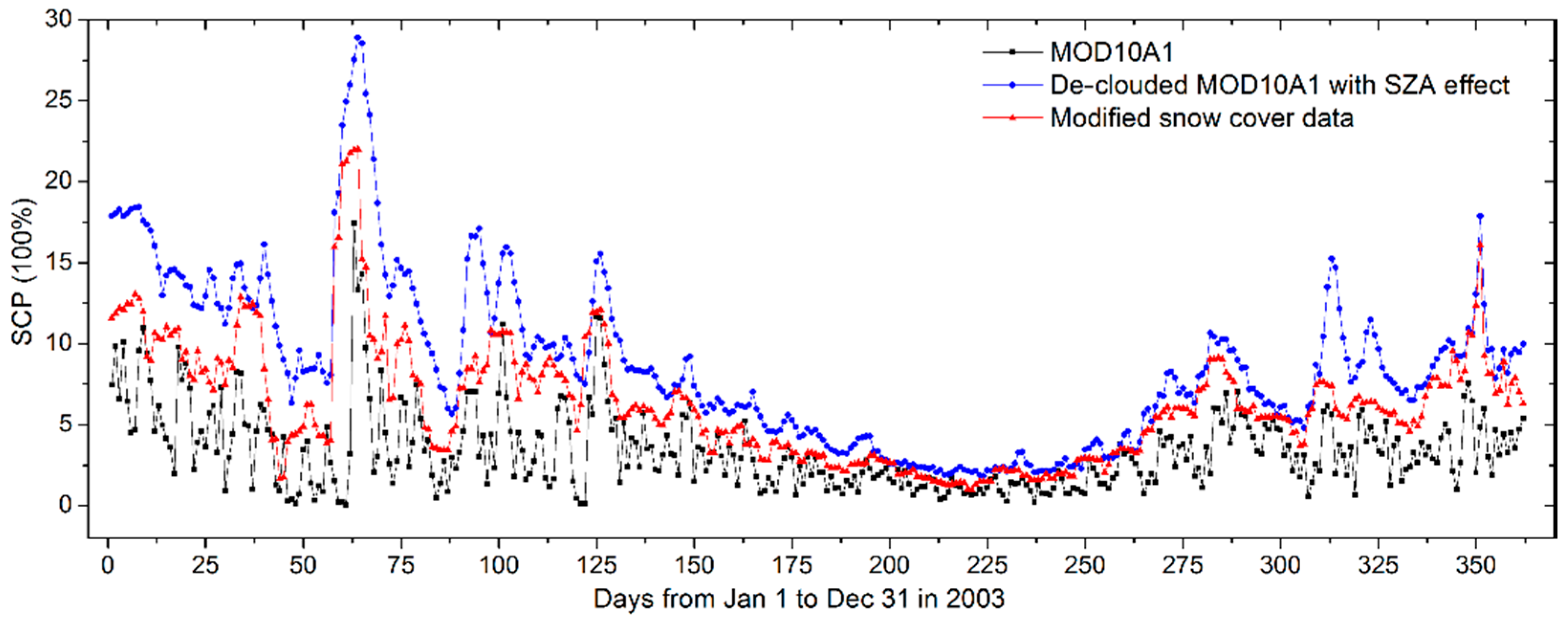
We used this multiday refilling method to modify the MOD10A1 data for 2003 and examined the changes in daily SCP (
Figure 8). The SCP values for de-clouded MOD10A1 data were consistently higher than the calculated SCP values obtained from the original MOD10A1 data, whereas the SCP values for the modified snow cover data were lower than those for the de-clouded SCP. Annual SCP average values for the MOD10A1 data, de-clouded MOD10A1 data, and modified MOD10A1 data were 3.42%, 8.69%, and 6.24%, respectively. We can therefore reasonably assume that the differences between the de-clouded and modified data were due to overestimation caused by a larger SZA, which clearly had a significant influence. The results also revealed that the modified data would considerably improve the accuracy of MOD10A1-based interpretations.
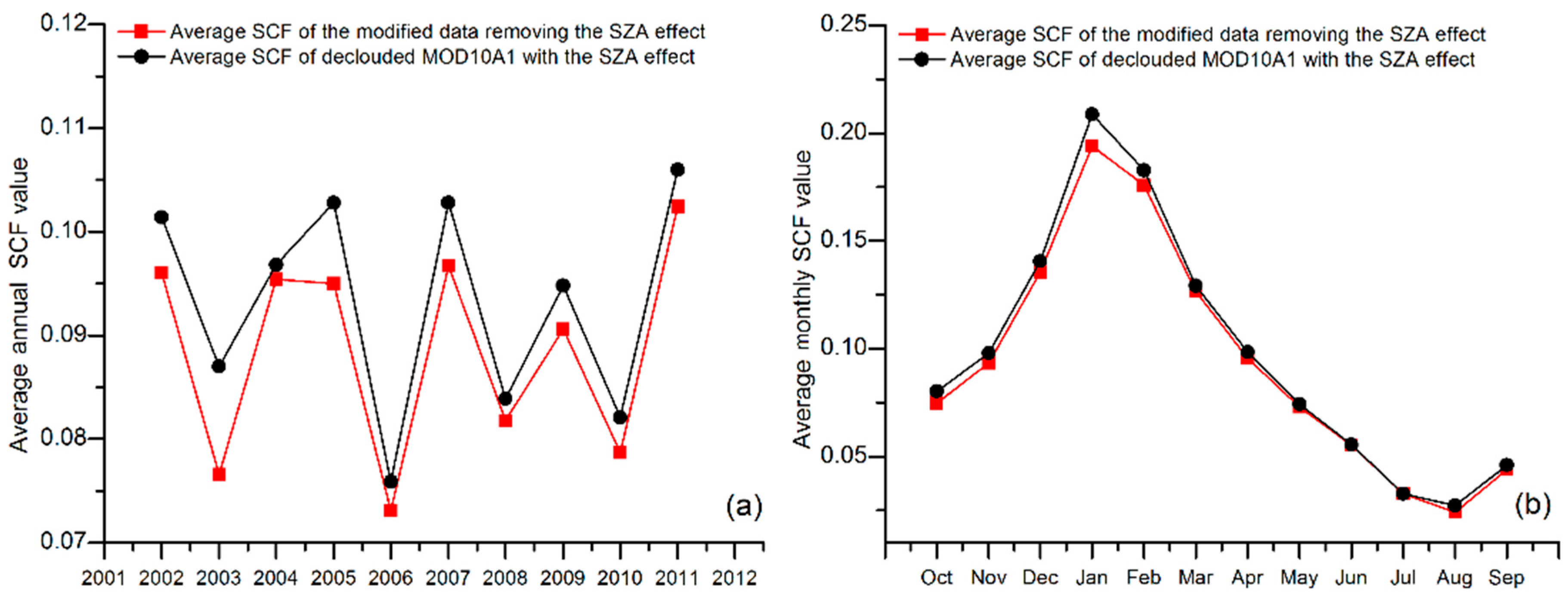
The SCF data for the 10 years between 2002 and 2011 were also used to evaluate the SZA effect.
Figure 9a shows the annual average SCF values in the Tarim River Basin (2002–2011) before and after removing pixels with SZA values larger than the threshold value. The SCF is defined as the number of times that a MODIS pixel is classified as snow covered relative to the total number of valid observations obtained during a certain period [
33]; thus, it is a spatiotemporal measure of snow cover distribution. These data show that the average SCF of the modified snow cover data decreased relative to that for the average de-clouded MOD10A1 SCF data over this 10-year period. The maximum difference between the average SCF values was a decrease from 0.087 to 0.076 in 2003, which was a relative change of 12.6%, whereas even the minimum change of SCF in 2004 had a relative change of 1.5%. The average decrease was 5.4%. The average SCF values for the same month in each of the 10 years are shown in
Figure 9b, which shows that the monthly SCF difference has a clear seasonal pattern. The SZA effect during periods without snow melting was larger than that during snow-melting periods, with a maximum relative difference of 7.6% in January. Even in April—the snow-melting period—there was a non-negligible difference of 3.03%. The only month that exhibited no difference was July, which also indicated that our results are real and meaningful. The monthly decrease in the average SCF values reached 4.3%, which approached the results obtained for the annual decrease.
4.6. Comparison and Validation of Modified MOD10A1 Data with HJ-1A/B Data
HJ-1A/B is a new generation of small, Chinese, civilian, earth-observing optical remote sensing satellites that have medium/high spatial resolution, high temporal resolution, hyperspectral resolution, and wide bandwidth. They are equipped with a wide-coverage multispectral charge-coupled device camera that has a nadir pixel resolution of 30 m and a field-of-view width of 360 km [
34]. Multitemporal and multispectral data provided by HJ-1A/B can provide daily snow cover classification maps; thus, we utilized these images in our work as reference materials because of their superior resolution in both space and time.
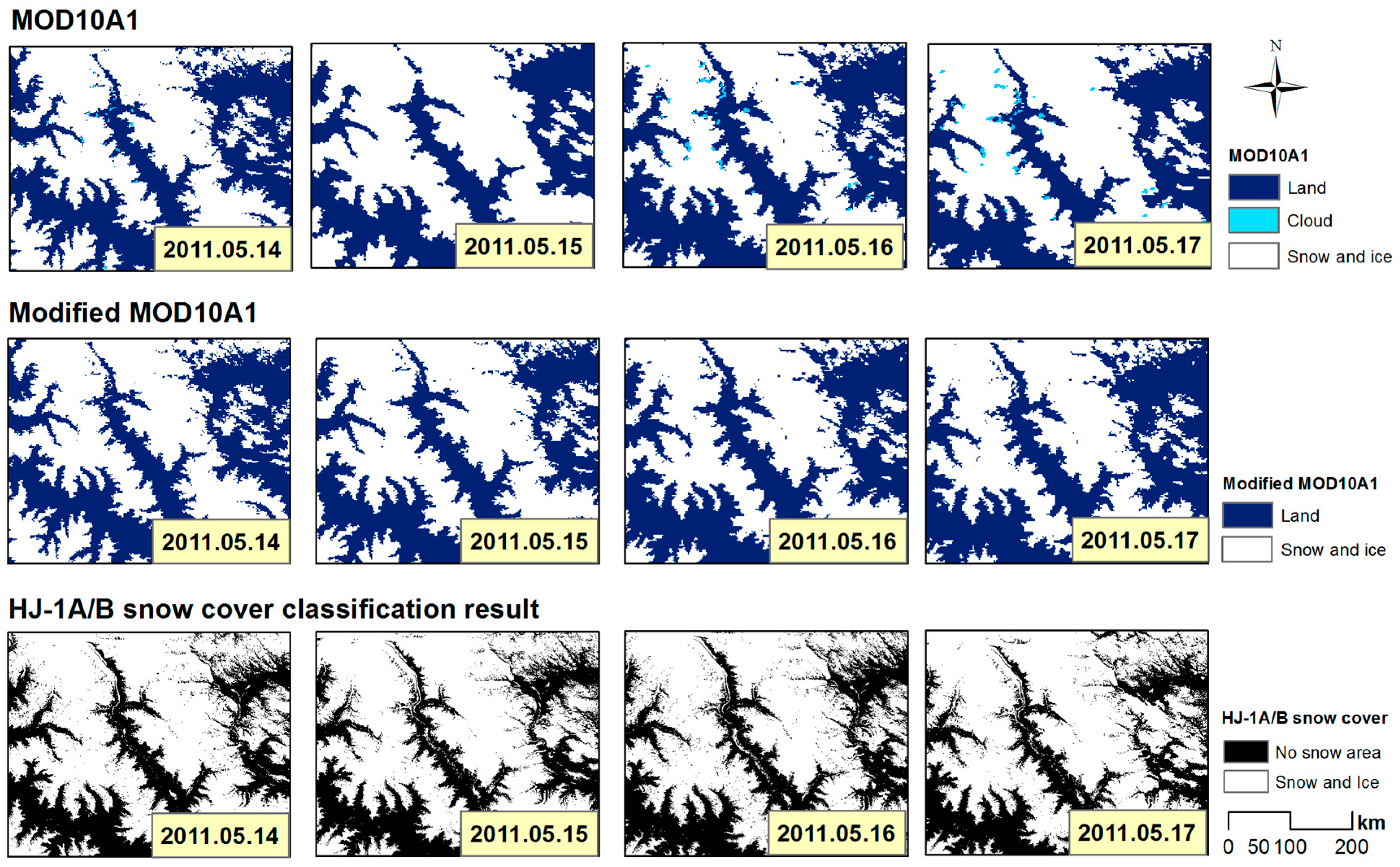
Figure 10 shows a graphical comparison of snow-covered areas derived from raw MOD10A1 data, modified MOD10A1 data, and HJ-1A/B data for four consecutive days from 14–17 May 2011. In comparison with data from the original MOD10A1 dataset, visual inspection shows that the modified MOD10A1 data have clearer snow cover outlines and they are more consistent with the snow cover results calculated from the HJ-1A/B data. In particular, the blurred edges of snow cover on the images of 15 and 17 May disappear following our modification, and the minor amount of cloud cover was accounted for on each daily image.
Daily SCP values, the changes in these SCP values, their overall accuracies, and the calculated rates of increase of the overall accuracy for each of these three datasets are given in
Table 2. By taking the HJ-1A/B SCP values as a reference, the decrease in SCP after modification of the MOD10A1 dataset indicated that snow cover overestimation due to a large SZA was especially important on 15 and 17 May, 2011. The overall accuracies of the MOD10A1 data for the four days were 67.75%, 63.28%, 66.68%, and 62.86%, respectively; the overall accuracies of the modified snow cover dataset were 68.14%, 67.96%, 67.20%, and 66.63%, respectively; and the overall accuracies for each improved by 0.39%, 4.68%, 0.52%, and 3.77%, respectively. The minor increases in the overall accuracies on 14 and 16 May were likely due to the occurrence of low SZA values that were below the threshold outlined above, whereas the clear increases in the overall accuracies on 15 and 17 May can be attributed to the modification of the snow cover overestimation pixels that had a large SZA.
In order to demonstrate more convincingly the effects of this modification, we selected 30 snow-covered areas in 2011 that had SZA values larger than the optimal threshold of 22.37°, and we compared the overall accuracies calculated for raw MOD10A1 data and modified MOD10A1 snow cover data using HJ-1 A/B as a reference. These results are given in
Table S1 in the supporting material and they show that the overall accuracies of the modified dataset all increased in comparison with the overall accuracies of the original MOD10A1 data. These data showed an average increase of 4.11% in the accuracy, which we take as confirmation that our modified snow cover dataset is both practical and effective.
5. Discussion
We used reference SCA data obtained from the HJ-1 A/B satellite over several consecutive days to demonstrate a relationship between the expanded snow cover within the MOD10A1 dataset and high SZA values. Ten years’ continuous hydrological data from MOD10A1 were used to develop SZA sensitivity relationships for both individual points in time and for all suitable days throughout a melting season. This enabled comparisons between SCA calculations made using different sensors. Scatter plots for five subwatersheds of the Tarim River Basin showed that a large SZA directly correlated with an overestimation of snow cover, and that a linear relationship existed between the increased SZA and SCA.
Previous investigations into the effect of an increased SZA have focused mainly on the sensitivity of SZA to vegetation indices. For example, a significant SZA effect was reported for a normalized difference vegetation index at a forest site (NDVI), which indicated that the former affected the latter by up to 15% [
35]. In the case of the NDVI, the red band has been reported much more sensitive to SZA than the near-infrared band [
36]. In our study, the green band was found significantly more sensitive to SZA than the near-infrared band, which caused the NDSI to show acute SZA sensitivity. The different responses that snow or vegetation show to SZA must be investigated further and it is important to note that the SZA effect is not limited to MOD10A1 data. Together, these findings indicate that SZA effects would not cancel each other out and that the NDSI/NDVI would show sensitivity to SZA. This is because a normalized difference index will not eliminate SZA sensitivity if both spectral bands in the index have different SZA sensitivities. In any case, when dealing with an index that is an arithmetic combination of reflectance in several bands, the magnitude of the SZA effect is also dependent on both the arithmetic form of the index and the changes in the actual index value for different canopy components that might be viewed at different angles.
A nadir SZA area was used as a reference in our work to establish the minimum sensitive angle that caused overestimation of snow-covered pixels. In the Tarim River Basin, this angular threshold was determined to be 22.37°, which is close to that of MODIS Persistent Ice (MODICE). MODICE determines the annual minimum amount of exposed snow and ice cover by searching each pixel’s time series of MODSCAG retrievals for a given snow-free date, and it only includes MODSCAG retrievals for pixels that have an SZA of less than or equal to 25°. The existence of a regional difference of this angular threshold is interesting and worthy of further study. Where coincident data exist, particular effort could be focused on comparisons and analyses that extend beyond the Tarim River Basin for many years.
The multiday filling method used herein has the dual function of replacing pixels with large SZA values with reliable SCA data and removing the extensive cloud cover from the MOD10A1 dataset. The paired-date method was applied to investigate the existence of overestimation of snow cover in MOD10A1 data and to identify a linear correlation between increases in SCP and SZA. An increase in the overall accuracy also showed that our modified product constituted a significant improvement on the original dataset, and further verified the existence of the SZA overestimation effect. However, other influential factors should also be taken into consideration, such as the effects of topography, solar geometry, time of acquisition, error in mapping from projection, and the shading effect caused by the difference between forward- or back-scatter directions [
37,
38,
39]. In particular, the shading effect in mountainous areas is of prime importance, because considerable subpixel topographic variation occurs within a given visible area. Nonetheless, this is likely less important for our study because of the low-resolution sensor used to collect the MOD10A1 data. The daily fluctuation of the solar zenith angle in the Tarim River Basin was more stable than that of the SZA due to the fixed acquisition time. An improvement to the sun-angle correction was also made in MOD10A1 to correct for within-orbit variation, as seen in the ground-based control point residuals [
40]. As such, we did not consider these factors in this study, although long-term seasonal changes in the solar zenith angle will cause it to increase, which will also affect these variations.
6. Conclusions
In this study, the overestimation of snow cover by MOD10A1 within the Tarim River Basin was verified to be correlated with high values of SZA and the mechanism responsible for the SZA effect was analyzed. A facile modification technique was proposed to modify the MOD10A1 dataset. The following conclusions can be drawn from this work:
(i) A clear overestimation of SCA resulting from high SZA values was confirmed in various regions of the Tarim River Basin. Hydrological statistics (e.g., amount of snow cover) spanning 10 years in the region corroborated the existence of a positive correlation between high SCP and high SZA during snow-melting periods, which was documented from five different subwatersheds in the region.
(ii) Analysis of the mechanism responsible for this SZA effect showed that reflectance at Band 4 and Band 6 of MODIS changes unevenly throughout the same range in SZA variation, which led to an increase in NDSI and an overestimation of SCA in pixels with large SZA values. A threshold SZA value of 22.37° was determined as the minimum at which a statistically significant response in snow cover overestimation occurred.
(iii) By adopting an appropriate SZA threshold and using a multiday refilling method, a modified snow cover dataset could be produced with ease. After removal of the cloud cover, the calculated decreases in SCF and SCP from this modified snow cover data further indicated the importance of this SZA effect.
(iv) Data collected by the HJ-1A/B satellite (with pixel resolution of 30 m) was compared with the snow cover data within our modified MOD10A1 dataset (with pixel resolution of 500 m). It showed that the removal of areas of overestimation led to an increase in the accuracy of the calculated snow cover from about 63% to 67%. This increase indicated that our modified dataset could be used for reliable daily analysis of snow cover identification by minimizing the detrimental effects of SZA.


