Estimation of Boreal Forest Attributes from Very High Resolution Pléiades Data

Abstract

In this study, the potential of using very high resolution Pléiades imagery to estimate a number of common forest attributes for 10-m plots in boreal forest was examined, when a high-resolution terrain model was available. The explanatory variables were derived from three processing alternatives. Height metrics were extracted from image matching of the images acquired from different incidence angles. Spectral derivatives were derived by performing principal component analysis of the spectral bands and lastly, second order textural metrics were extracted from a gray-level co-occurrence matrix, computed with an 11 × 11 pixels moving window. The analysis took place at two Swedish test sites, Krycklan and Remningstorp, containing boreal and hemi-boreal forest. The lowest RMSE was estimated with 1.4 m (7.7%) for Lorey’s mean height, 1.7 m (10%) for airborne laser scanning height percentile 90, 5.1 m²·ha⁻¹ (22%) for basal area, 66 m³·ha⁻¹ (27%) for stem volume, and 26 tons·ha⁻¹ (26%) for above-ground biomass, respectively. It was found that the image-matched height metrics were most important in all models, and that the spectral and textural metrics contained similar information. Nevertheless, the best estimations were obtained when all three explanatory sources were used. To conclude, image-matched height metrics should be prioritised over spectral metrics when estimation of forest attributes is concerned.

1. Introduction

Accurate information about the forest is essential for making well-founded management decisions. The necessary information has traditionally been obtained from field visits and sample-based forest inventories [1]. To improve the accuracy, more samples are collected. However, field measurements are expensive and time-consuming, and the method is inefficient on larger scales. Remote sensing techniques complement and can further increase the value of the field inventoried data, with large detailed coverages at acceptable costs [2,3,4]. The combined use of remote sensing data and field based measures has been evaluated for estimations of common forest attributes, such as Lorey’s mean height, H_L (the tree height is weighted with its basal area, BA), stem diameter, stem volume (VOL), and biomass [5,6,7,8].

There are numerous remote sensing techniques available, with their respective (dis-)advantages. For the past 10 years, airborne laser scanning (ALS) has been considered the most accurate remote sensing technique for forest estimations [5,6,7]. The strength of ALS is its ability of reconstructing the forest at a very high level of details in three dimensions (3D). However, it is a rather expensive technique, which restricts its use for frequent acquisitions and larger areas. The airborne platform is, moreover, not directly available to most people, and requires arduous practicalities to be managed, which might limit its use in small applications, for example by private forest owners.

To cope with these problems related to costs, availability, and practicalities, image-matching techniques may be an alternative. In its simplest form, the same objects (pixels) are detected in at least two images, acquired from different positions in space, and, based on the appeared differences (parallaxes) and the known positions for the acquisitions, the x, y, z coordinates can be computed for the objects. Digital surface models (DSMs) can be computed from air- and space-borne images, which in combination with an accurate digital terrain model (DTM) can be used to derive forest attributes [9,10,11]. Typical 3D attributes, e.g., forest height and some volumetric metric, can be derived at sufficient quality (better than traditional field inventory methods currently used by many forest companies), and the spectral information can be combined to further improve model accuracies [10,12]. Airborne photogrammetry is an old, well-known technique used in many countries including Sweden, but it suffers from high costs similar to those of ALS. However, it has the advantage of also providing spectral data, and promising results for estimation of forest attributes have been reported by, e.g., Bohlin et al. [13], Stepper et al. [14], and White et al. [11]. An attractive alternative to the expensive aerial platform is satellites, which provide frequent acquisition with large coverage at reasonable cost and short repetition intervals. New stereo acquisitions can simply be ordered directly via the Internet. Moreover, the resolution of the very high resolution (VHR) satellite sensors available today is similar (~0.5 m ground sampling distance) to imagery from airborne platforms flown at ~5000 m elevation (commonly used for photogrammetry). Additionally, the VHR sensors often provide more and narrower spectral bands, facilitating complex analyses. The set of optical VHR sensors (including, e.g., GeoEye-1, Ikonos, Pléiades and WorldView-2), are normally steerable sensors that make stereo or even tri-stereo acquisitions available from a single overpass, which is crucial to obtain two cloud-free images within a short temporal interval.

Thus far, a limited number of studies have used optical VHR sensors for image matching and estimation of forest attributes. However, they have covered different conditions. Kayitakire et al. [15] used textural metrics from Ikonos-2 imagery to retrieve different forest attributes in temperate forest with mainly spruce in Belgium. They predicted top height with 2.2 m RMSE (10%), stocking (stems·ha⁻¹) with 276 stems·ha⁻¹ (29%), and BA with 7.1 m²·ha⁻¹ (16%). St-Onge et al. [16] evaluated the accuracy of average dominant forest height (1.7 m RMSE, 8%) and above-ground biomass (AGB; 71 tons·ha⁻¹, 47%) at plot level, based on an Ikonos stereo pair and an ALS DTM at a Canadian boreal test site located in Quebec. The coefficient of determination (R²) reached 0.91 and 0.79, respectively. WorldView-2 imagery has been involved in studies from different biomes around the globe. Ozdemir and Karnieli [17] evaluated numerous structural parameters in a dryland forest plantation with mostly pine trees in Israel. They found that WorldView-2 textural metrics could be used to estimate BA with 1.8 m²·ha⁻¹ RMSE (17%), stocking with 110 stems·ha⁻¹ (29%) and VOL with 27 m³·ha⁻¹ (44%), for 29 plots of 30 m × 30 m. One conclusion was that further studies should cover different ecological regions. Straub et al. [18] used Cartosat-1 and WorldView-2 stereo images to estimate growing stock (VOL) in a mixed German temperate forest. They found the RMSE for VOL to be 162 m³·ha⁻¹ (50%) for Cartosat-1 and 143 m³·ha⁻¹ (44%) with WorldView-2 data at plot level. Similarly, Shamsoddini et al. [19] used WorldView-2 multispectral data to map pine plantation structures in a temperate forest in New South Wales, Australia. They investigated several combinations of spectral and height derivatives to explain tree height, diameter, VOL, BA, and stocking. Their final models were combinations of different spectral derivatives, height- and textural metrics. The RMSEs were 1.9 m (8%) for tree height, 4.1 cm (14%) for diameter, 90 m³·ha⁻¹ (30%) for VOL, 7.7 m²·ha⁻¹ (23%) for BA, and 151 trees·ha⁻¹ (25%) for stocking. They pointed out that textural features perform better than spectral information for estimating forest attributes. Perko et al. [20] examined the mapping potential of Pléiades stereo and triplet data at two mountainous test sites, located in Trento, Italy, and Innsbruck, Austria. Their focus was geo-locational accuracy and height accuracy compared to ALS data. They found it necessary to manually assign ground control points (GCPs) to achieve sub-pixel accuracy and, moreover, the image matching computed from an image triplet was preferred over matching from only an image pair.

Immitzer et al. [21] used WorldView-2 stereo images in combination with national forest inventory data to map growing stock wall-to-wall in a temperate forest in Bavaria, Germany. They found the combination of using both spectral and height data to be the best, corresponding to the R² being 0.53 and the RMSE for VOL was 120 m³·ha⁻¹ (32%) at plot level. Maack et al. [22] used WorldView-2 imagery for a German test site and Pléiades data for a test site located in Chile in order to estimate AGB. They emphasized the evaluation of combining spectral derivatives, textural metrics, in addition to image matched height metrics. They found the highest model performance when combining either height metrics and spectral derivatives, or height metrics and textural metrics. The model combining height metrics and spectral derivatives had 47 tons·ha⁻¹ (24%) RMSE at the German test site and 59 tons·ha⁻¹ (36%) at the test site in Chile. Both Immitzer et al. [21] and Maack et al. [22] obtained their main model contributions from the height metrics, while the spectral/textural contributions were rather limited. In Finland, Yu et al. [7] used WorldView-2 data to evaluate forest attributes in boreal forest. They compared numerous remote sensing techniques to estimate AGB (22 tons·ha⁻¹ RMSE, 16%), VOL (43 m³·ha⁻¹, 16%), BA (4.3 m²·ha⁻¹, 16%), basal area-weighted mean diameter (3.4 cm, 13%), and H_L (1.4 m RMSE, 7%) at plot level. They found the upper height percentiles 80 to 100 (p80 to p100) to be the most powerful predictors for H_L and mean diameter, while p30, mean height, and a canopy closure metric were most important for estimation of VOL and AGB.

From the review of past articles, few papers [20,22] have evaluated Pléiades satellite data for forestry purposes. The objective for this study is therefore to examine the use of Pléiades satellite data for estimating forest attributes in boreal forest, when a high-resolution DTM from ALS is available. Specifically, the explanatory capacity of using spectral data and texture metrics in addition to image matched height metrics is assessed. The evaluated forest attributes are H_L, ALS height p90, BA, VOL, and AGB. The attribute ALS p90, highly correlated to H_L, is included to facilitate comparisons to other sensors, and to regions where field data are not available. For comparison, the forest attributes are also estimated solely from ALS data.

2. Materials and Methods

2.1. Test Sites

Two Swedish test sites located in the boreal forest zone were used (Figure 1). The first test site is the Krycklan river catchment area, located in northern Sweden (64°16′N, 19°46′E). The forest is managed both by small private forest owners and large forest companies. The prevailing tree species were Scots pine (Pinus sylvestris; 44% volume, mainly in dry upslope areas), Norway spruce (Picea abies; 39% volume, mainly in wetter, low-lying areas), and birch (Betula pendula and Betula pubescens; 17% volume, in the riparian forest along larger streams). The stands contain mainly homogenous one-layered forest with a field layer consisting of different forbs, bilberry (Vaccinium myrtillus) and grasses (e.g., Deschampsia flexuosa). The region is hilly with elevations between 125 m and 350 m above sea level and slopes up to 61°.

The second test site is Remningstorp, located in southern Sweden (58°30′N, 13°40′E), which comprises about 1200 ha of productive managed forest land. The prevailing tree species were Scots pine (18% volume), Norway spruce (68% volume), and birch (13% volume). The dominant soil type is till (i.e., a mixture of glacial debris) with a field layer consisting of different forbs, bilberry, and grasses. In denser old spruce stands, the field layer is absent. It is a rather flat region with moderately varying ground elevations between 120 m and 145 m above sea level and slopes up to 21°.

2.2. Field Data

A systematic grid of circular plots with 10 m radius was distributed at both test sites. In Remningstorp 219 plots with about 200 m spacing were inventoried in the fall 2014. In Krycklan 326 plots with about 350 m spacing were inventoried in the fall 2015. The distribution of plots within the test sites is illustrated in Figure 2. The plot locations were measured using a Trimble GeoExplorer 6000 GeoXR, and all trees with a diameter at breast height (DBH) ≥ 0.04 m were calipered. The height was measured on a random sub-sample of about 10% of the trees, using a hypsometer. The tree height distribution at the two test sites is presented in Figure 3 and a few key statistical measures are presented in

Table 1. Properties for the reference dataset. SD denotes standard deviation.

Test Site	Forest Attribute	Mean	Min	Max	SD	Unit
Krycklan	HL	14.6	4.42	24.6	3.48	m
Krycklan	ALS p90	13.9	3.36	26.5	3.81	m
Krycklan	BA	23.2	1.51	62.8	8.80	m2·ha−1
Krycklan	VOL	288	7.45	1030	151	m3·ha−1
Krycklan	AGB	102	5.29	353	51.9	tons·ha−1
Remningstorp	HL	18.7	6.04	27.9	4.59	m
Remningstorp	ALS p90	16.8	4.23	26.5	4.51	m
Remningstorp	BA	26.5	1.38	66.7	10.5	m2·ha−1
Remningstorp	VOL	250	6.13	782	136	m3·ha−1
Remningstorp	AGB	143	3.67	421	71.8	tons·ha−1

.

2.3. Remote Sensing Data

ALS height data were collected for the test sites approximately the same time as the field and satellite data. Remningstorp was scanned on 4 August 2014 with a Riegl LMS 680i laser scanner at 240 kHz PRF and with >20 points m⁻² density. The wavelength was 1550 nm. Krycklan was scanned on 22 and 23 August 2015 with a Titan L359 laser scanner at 300 kHz PRF and with >20 points m⁻² density. The wavelength was 1064 nm.

The DTM utilized was produced by the Swedish National Land Survey (Lantmäteriet) from ALS data, with 0.5 m⁻² point density, and 2 m pixel size [23,24].

Ortho-photographs with 0.5 m resolution were provided by Lantmäteriet, and used for measuring of GCPs.

Optical satellite images were acquired from the Pléiades satellites in 2015. The images were delivered as pansharpened along-track stereo triplets in four bands (blue, green, red, near infrared), with a spatial resolution of 0.5 m and with a primary processing level, which contains corrections for radiometric and sensor distortions, using internal calibration parameters, ephemeris, and attitude measurements. The details of the satellite images are given in

Table 2. Acquisition properties for the satellite images. Ground sampling distance (GSD).

Test Site	Image No.	Incidence Angle Along-Track (°)	GSD Across/Along (m)	Date
Remningstorp	1	−13.2	0.77 × 0.80	4 April 2015
Remningstorp	2	1.33	0.75 × 0.75	4 April 2015
Remningstorp	3	14.3	0.72 × 0.75	4 April 2015
Krycklan	1	−13.3	0.74 × 0.73	17 August 2015
Krycklan	2	−8.15	0.72 × 0.72	17 August 2015
Krycklan	3	11.8	0.75 × 0.76	17 August 2015

,

Table 3. The spectral information of Pléiades images.

Band	Pixel Size (m)	Wavelength Range (nm)	Centre Wavelength (nm)
Blue	0.5	430–560	495
Green	0.5	500–617	559
Red	0.5	590–722	656
Near-infrared	0.5	740–945	843

and

Table 4. Sun elevation angles (°).

Image Pair	Sun Azimuth	Sun Elevation
Krycklan	174.65	39.27
Remningstorp	164.27	36.45

.

2.4. Data Processing

The different data sources were handled in different ways to derive the data that were extracted plot-wise. The processing chain is illustrated in Figure 4, and will be described in the following subsection.

2.4.1. Field Data Processing

The single-tree field data were used to compute plot-wise forest attributes. Linear regression was used to assign height values to all inventoried trees at the respective test sites. H_L was computed plot-wise, according to

$$H_L=\frac{{\displaystyle \sum }BA\times h}{{\displaystyle \sum }BA},$$

(1)

where h is the tree height. The VOL was computed using Brandel’s functions, derived for Swedish forest [25]. The AGB was computed using modified Marklund functions [26,27]. The VOL and AGB functions use h and DBH as explanatory variables. Field plots located on mires and within 10 m from clear-cuts were removed. Out of the 326 field measured plots in Krycklan, and 219 in Remningstorp, 275 plots and 169 plots were used, respectively.

2.4.2. ALS Data Processing

The ALS data were classified, normalized (converted to heights above the ground), and filtered for noise (points > 40 m were dropped to avoid errors from, for example, birds) using the software Lastools (http://rapidlasso.com/lastools). Then plot-wise height metrics were extracted above a 1.37 m height cutoff to avoid undervegetation. The height metrics extracted were mean height, canopy cover (COV), height percentiles 20, 50, 60, 70, 80, 90, 95, 99, and 100, kurtosis and skewness, and SD.

2.4.3. Geometric Corrections

Pléiades panchromatic imagery is reported to possess a geo-locational accuracy of 8.5 m CE90 (circular error at 90% confidence) at the nadir direction and 10.5 m CE90 within 30° off-nadir, when applying the provided rational polynomial coefficient (RPC) model [28]. However, for the kind of purposes this study examines, sub-meter accuracy is important. Therefore, about 10 GCPs (sufficient according to [20]) were manually distributed across the respective image within the triplet. Ground truth was obtained from ortho-photographs and the ALS DTM. The resulting accuracies are presented in

Table 5. Accuracy analysis after geometric correction using GCPs.

Test Site	RMSE m (x)	RMSE m (y)	RMSE m (z)	GCPs
Krycklan	0.59	0.61	2.2	11
Remningstorp	0.68	0.29	1.5	9

. The GCPs were used both for geocoding of the image matched data and for ortho-rectification of the individual images.

Because of the hilly conditions at the Krycklan test site, some topographic corrections were considered. Both the cosine correction and the Minnaert correction were evaluated, but none of them improved the overall accuracy of the estimated attributes and, hence, these corrections were neglected [29].

2.4.4. Image Matching

The image matching was computed with the software Remote Sensing Graz (RSG; http://www.remotesensing.at/en/remote-sensing-software.html). It used epipolar rectification of the images based on optimized sensor models, derived from the GCPs. Hence, a pre-defined point in the reference image can be found along a horizontal line in the search image. A semi-global image matching, similar to Hirschmüller [30], was used to compute disparities for each pixel for the three stereo pairs (images 1-2, 1-3, and 2-3). The result yields two dense disparity maps for each image pair, one from the reference to the search image and one vice versa. Finally, spatial point intersection was applied to calculate ground coordinates in a least-squares manner out of the image matching disparities. The final step resulted in six 3D point clouds (three image pairs, both forward and backward matching) that were merged together, from which plot-wise metrics were extracted. The employed procedure is very similar to the more comprehensive description in Perko et al. [20]. The same metrics as for the ALS data were extracted, but no height cutoff was found to be necessary. An extraction of one of the point clouds is illustrated in Figure 5.

2.4.5. Spectral Derivatives

The ortho-rectified satellite images were visually compared to ortho-photographs for the respective test sites and the most nadir satellite image (close to 0 degrees look angle) was found most similar and therefore most suited to use for extraction of the spectral data. The average spectral values for all four available bands were extracted plot-wise. The bands are normally highly correlated and therefore to improve data handling and analysis, principal component analysis (PCA) was applied to the data. This linear orthogonal transform causes the principal components (PCs) to be orthogonal and minimizes the cross-correlation. In practice, the first PC (PC1) generally represents the dominant signal while the remaining principal components (PC2 to PC4) increasingly possess more noise. However, it is highly dependent on the application, and thus the first PC was not always necessarily included in every regression analysis.

2.4.6. Textural Metrics

In order to not only average the spectral values within plots, but also consider the inter-spatial relations, statistical textural analysis can be used. A few studies have shown these to be of similar importance as the image-matched height metrics [21,22] and some other are based purely on textural analysis [15,17,19]. The literature honour co-occurrence analysis, and specifically the grey-level co-occurrence matrix (GLCM) method with its related attributes. It is a way of extracting second-order statistical texture features, while the spectral derivatives can be considered first-order features, as they do not consider pixel neighbour relationships. GLCM was developed by Haralick, Shanmugam, and Dinstein [31], and has commonly been applied in remote sensing studies [15,17,19,22,32,33]. Ten common textural attributes (contrast, dissimilarity, homogeneity, second moment, energy, max probability, entropy, average, variance, and correlation) were computed using the Sentinel Application Platform (SNAP; http://step.esa.int/main/toolboxes/snap) commissioned by the European Space Agency (ESA). The computations were carried out with four different window sizes (5 × 5, 7 × 7, 9 × 9 and 11 × 11 pixels), as these features can be affected by for example, image resolution, forest characteristics, and environmental conditions at the time of acquisition. The average textural values for the 10 GLCM features were extracted plot-wise for respective bands, which in total gave 40 explanatory variables. To address correlations and increase the signal-to-noise ratio, PCA was also applied to these data and the first seven PCs were selected as input in the empirical models. The cumulative proportion for the seven PCs was >0.98, and no single additional PC could support important improvements in the explanation of the data variation.

2.5. Empirical Modelling and Validation Assessment

Multiple linear regression was used for determining the relationship between the different extracted attributes and metrics described in Section 2.4.4, Section 2.4.5 and Section 2.4.6, and the field- and ALS-based forestry metrics described in Section 2.4.1 and Section 2.4.2. The explanatory variables were chosen to increase accuracy (lower RMSE and higher adjusted coefficient of determination; R²). In case of residual plots that showed a dependence or trend for a specific variable, some simple transformations were evaluated (e.g., different powers or logarithmic transformations). The suitable explanatory variables were tested in four groups: (1) Only height metrics; (2) Only spectral metrics (PCs); (3) Only textural metrics; (4) All explanatory variables (from all groups). The complete models with their significance levels are described in

Table A1. Coefficients and significance levels (*** = p ≤ 0.001, ** = p ≤ 0.01, * = p ≤ 0.05) for the complete models from Group 4. α0 denotes the intercept while the following α denotes the explanatory variables in the same order.

Test Site	Estimated Variable	Explanatory Variables	α0	α1	α2	α3	α4	α5
Krycklan	HL	H100 + tPC2 + tPC3 + sPC1	8.73 ***	0.557 ***	−2.59 ***	−4.47 ***	−1.24 ***
Remningstorp	HL	Hmean + HSD	7.28 ***	0.828 ***	0.565 ***	0.145 *	0.776 ***	−0.702 ***
Krycklan	ALS p90	H100 + tPC1 + sPC2	5.69 ***	0.720 ***	−0.109 ***	0.825 ***
Remningstorp	ALS p90	H100 + Hmean + HSD	3.46 ***	0.182 **	0.657 ***	0.725 ***
Krycklan	BA	Hmean + tPC5 + tPC7 + sPC1 + sPC2	12.0 ***	1.91 ***	−0.970 ***	−4.22 ***	−1.30 ***	−6.33 ***
Remningstorp	BA	Hmean2 + sPC2 + tPC1	14.6 ***	−4.59 ***	0.0637 ***	0.445 *
Krycklan	VOL	H1002.3 + Hmean + tPC1 + tPC2 + tPC3	100 ***	0.201 ***	23.6 ***	−16.9 ***	−73.1 ***	−115 ***
Remningstorp	VOL	Hmean2.6 + H100 + sPC2	49.3 *	0.121 ***	3.88 *	−51.9 ***
Krycklan	AGB	H1002.3 + tPC1 + tPC2 + tPC3	39.9 ***	0.0736 ***	−6.03 ***	−20.1 ***	−31.4 ***	7.11 ***
Remningstorp	AGB	Hmean2.7 + sPC2 + HSD + tPC3 + tPC4	61.0 ***	0.0505 ***	−23.8 ***	5.83 *	8.72 **	6.99 *

. For the respective groups, the suitable explanatory variables were selected, and only variables with significance (p-values < 0.05) were kept. The models were evaluated using leave-one-out cross-validation. A single sample from the original dataset is used to validate the model, which is fitted using all other samples in the original dataset. This is repeated so that each observation is used once for validation. The RMSE was computed as [34]:

$$RMSE=\sqrt{\frac{{{\displaystyle \sum }}_{i = 1}^n{({\widehat{X}}_i-X_i)}^2}{n}}$$

(2)

$$RMSE(\%)=\frac{RMSE}{\overline{X}},$$

(3)

where n is the number of plots, ${\widehat{X}}_i$ is the value estimated from Pléiades data for plot i, and $X_i$ is the target value for plot i. $\overline{X}$ represents the sampled mean for the variable in question. The adjusted coefficient of determination (R²) was computed according to Kvålseth [35].

3. Results

The overall results showed that the height metrics were most important in all estimations of the target variables. The models based on spectral data gave only a minor, yet significant, improvement in addition to the height metrics. The textural metrics had a similar information content compared to the spectral derivatives. However, in some models they did complement each other and therefore the overall model accuracy mostly improved when the suitable spectral and textural metrics were added as explanatory variables. Hence, the following results will focus on only height metrics (group 1,

Table 6. Results estimated from height metrics. Subscript numbers represent height percentiles, while the mean denotes the average and SD the standard deviation.

Test Site	Estimated Feature	Explanatory Variables	RMSE	RMSE (%)	R2
Krycklan	HL	H100	2.03 m	13.9	0.66
Krycklan	ALS p90	H100	1.68 m	12.0	0.81
Krycklan	BA	Hmean	5.63 m2·ha−1	24.4	0.58
Krycklan	VOL	H1002.3 + Hmean	80.1 m3·ha−1	27.9	0.72
Krycklan	AGB	H1002.3 + Hmean	29.2 tons·ha−1	28.6	0.69
Remningstorp	HL	Hmean + HSD	1.62 m	8.70	0.88
Remningstorp	ALS p90	H100 + Hmean + HSD	1.65 m	9.80	0.88
Remningstorp	BA	Hmean2	7.39 m2·ha−1	27.9	0.51
Remningstorp	VOL	Hmean2.6 + H100	75.8 m3·ha−1	30.3	0.70
Remningstorp	AGB	Hmean2.7	44.3 tons·ha−1	31.0	0.63

) and on the best combination of height metrics, spectral derivatives and textural metrics (group 4,

Table 7. Results estimated from height metrics, spectral (s), and textural (t) principal components (PCs). The abbreviations have the same meaning as before.

Test Site	Estimated Feature	Explanatory Variables	RMSE	RMSE (%)	R2
Krycklan	HL	H100 + tPC2 + tPC3 + sPC1	1.92 m	13.2	0.70
Krycklan	ALS p90	H100 + tPC1 + sPC2	1.62 m	11.6	0.82
Krycklan	BA	Hmean + tPC5 + tPC7 + sPC1 + sPC3	5.12 m2·ha−1	22.2	0.66
Krycklan	VOL	H1002.3 + Hmean + tPC1 + tPC2 + tPC3	72.9 m3·ha−1	25.4	0.76
Krycklan	AGB	H1002.3 + Hmean + tPC1 + tPC2 + tPC3	26.4 tons·ha−1	25.9	0.75
Remningstorp	HL	Hmean + HSD + tPC1 + tPC3 + tPC4	1.44 m	7.70	0.91
Remningstorp	ALS p90	H100 + Hmean + HSD	1.65 m	9.80	0.88
Remningstorp	BA	Hmean2 + sPC2 + tPC1	6.56 m2·ha−1	24.8	0.63
Remningstorp	VOL	Hmean2.6 + H100 + sPC2	66.4 m3·ha−1	26.6	0.77
Remningstorp	AGB	Hmean2.7 + sPC2 + HSD + tPC3 + tPC4	38.5 tons·ha−1	26.9	0.73

). For comparison, results from estimations based solely on ALS data are also presented in Section 3.3.

3.1. Performance of Models Based on Height Metrics

Table 6 shows how only one height metric (H₁₀₀ or H_mean) was used to describe H_L, ALS p90, or BA in Krycklan. In Remningstorp, the combination of these height metrics and also the standard deviation of the height contributed to the best models. The heights at both test sites were described fairly well, although the range of available heights is lower in Krycklan. The BA is a metric related to the forest density, and the results reveal that height metrics are not sufficient to describe this two-dimensional property as well as the H_L or ALS p90. Notable is that in Krycklan this target feature was best explained using the mean height (H_mean), while in Remningstorp the squared height was a better option. Both VOL and AGB, which are volumetric features, also required a transformed height metric, alternatively or in combination. The top height (H₁₀₀) or the mean height was normally raised to the power coefficient of about 2.5 in order to contribute the most to the models. In Remningstorp, the modelled power coefficients were generally slightly larger than for the Krycklan models, likely because of the taller and denser forest there.

3.2. Performance of Models Based on Height Metrics, Spectral Derivatives, and Textural Metrics

Most models were slightly improved when some spectral derivative and/or textural metric was added as an explanatory variable. Considering height as one-dimensional, BA as two-dimensional, and VOL/AGB as 3D, the improvements increased with higher dimensions. For example, the RMSE for height in Krycklan improved from 13.9% to 13.2% using the full model, while the VOL improved from 27.9% to 25.4% (Table 7). The image-matched heights describe the height well, while supplementary explanatory information improve the derivation of the other forestry metrics of higher dimensions. Figure 6 shows the scatter plots for the combined models (group 4, Table 7), where height metrics, spectral derivatives, and textural metrics were used as explanatory variables. The estimated heights followed the sampled heights (1 to 1 line) reasonably well (Figure 6a–d), but the forest in Krycklan is lower than in Remningstorp, which causes the relative RMSEs, especially, to be somewhat higher, albeit the absolute RMSEs were similar for the ALS p90 (1.68 m vs. 1.65 m; Table 7). The BA was also estimated similarly across sites, with relative RMSEs of 22.2% and 24.8%, respectively. The scatter plots get more dispersed at higher volume/biomass, which might indicate a decreased sensibility as the canopy closes. Nevertheless, the residuals were uniformly distributed along the entire range. There is a high similarity between the VOL and AGB results. The RMSEs were almost identical across test sites and across the features (25.4% vs. 26.6% for VOL, 25.9% vs. 26.6% for AGB; Table 7).

The height metrics computed from image matching were relatively homogenous, even though the tails in the distributions sometimes deviated significantly within single plots. Hence, the use of mean height (H_mean) or the top height (H₁₀₀) as an explanatory variable is of minor importance. If anything, the tendency was that image-matched heights from the higher height percentiles (50th to 100th) were more robust and better suited than lower height percentiles.

The spectral PCs (sPCs) were rather overlapping the textural PCs (tPCs) and therefore, normally either the first few sPCs and higher tPCs in combination, or vice-versa, were used as input, while the first few PCs from both sources were rarely used simultaneously (Table 7). The textural metrics were computed at four different window sizes (5 × 5 to 11 × 11) and the highest contribution (best model performance) was obtained with the largest window size (11 × 11). Hence, the textural contributions for the presented results are all derived from the textures computed with the 11 × 11 window.

3.3. Performance of Models Based on ALS Metrics

Table 8. Results estimated solely from ALS metrics. COV describes the ALS canopy cover. The other abbreviations have the same meaning as before.

Test Site	Estimated Feature	Explanatory Variables	RMSE	RMSE (%)	R2
Krycklan	HL	ALS p90 + COV	1.25 m	8.61	0.87
Krycklan	ALS p90		-	-	-
Krycklan	BA	ALS p602 + COV	4.32 m2·ha−1	18.7	0.76
Krycklan	VOL	ALS p902 + COV	60.4 m3·ha−1	21.1	0.84
Krycklan	AGB	ALS p902 + COV	22.4 tons·ha−1	22.4	0.82
Remningstorp	HL	ALS p90 + COV	1.60 m	8.59	0.89
Remningstorp	ALS p90		-	-	-
Remningstorp	BA	ALS p602 + COV	5.71 m2·ha−1	21.6	0.71
Remningstorp	VOL	ALS p902 + COV	68.6 m3·ha−1	27.5	0.76
Remningstorp	AGB	ALS p902 + COV	39.1 tons·ha−1	27.4	0.71

shows the performance for models based solely on ALS data. This is important to enable comparisons of the Pléiades-based methods (Section 3.1 and Section 3.2) with this commonly applied technique. The forest heights (H_L) were modelled with similar relative RMSE across the test sites when ALS data were used, and was lower than the best VHR model combination in Krycklan (8.61% vs. 13.2%), while it was slightly higher in Remningstorp (8.59% vs. 7.70%; Table 7 and Table 8). The BA was estimated with lower RMSE at both test sites (18.7% in Krycklan and 21.6% in Remningstorp; Table 8) compared to the models based on Pléiades data (22.2% and 24.8%; Table 7). Moreover, the BA was the only attribute where ALS p90 was replaced with ALS p60 in order to find a suitable model with significant explanatory variables. The VOL and AGB were both modelled with similar relative RMSE at the respective test sites. However, the RMSE was lower for the Krycklan models (21.1% and 22.4%) compared to the Remningstorp models (27.5% and 27.4%; Table 8). Like the Pléiades-based models, the ALS-based models for VOL and AGB included a transformed height variable, ALS p90², where coefficient 2 was found suitable.

4. Discussion

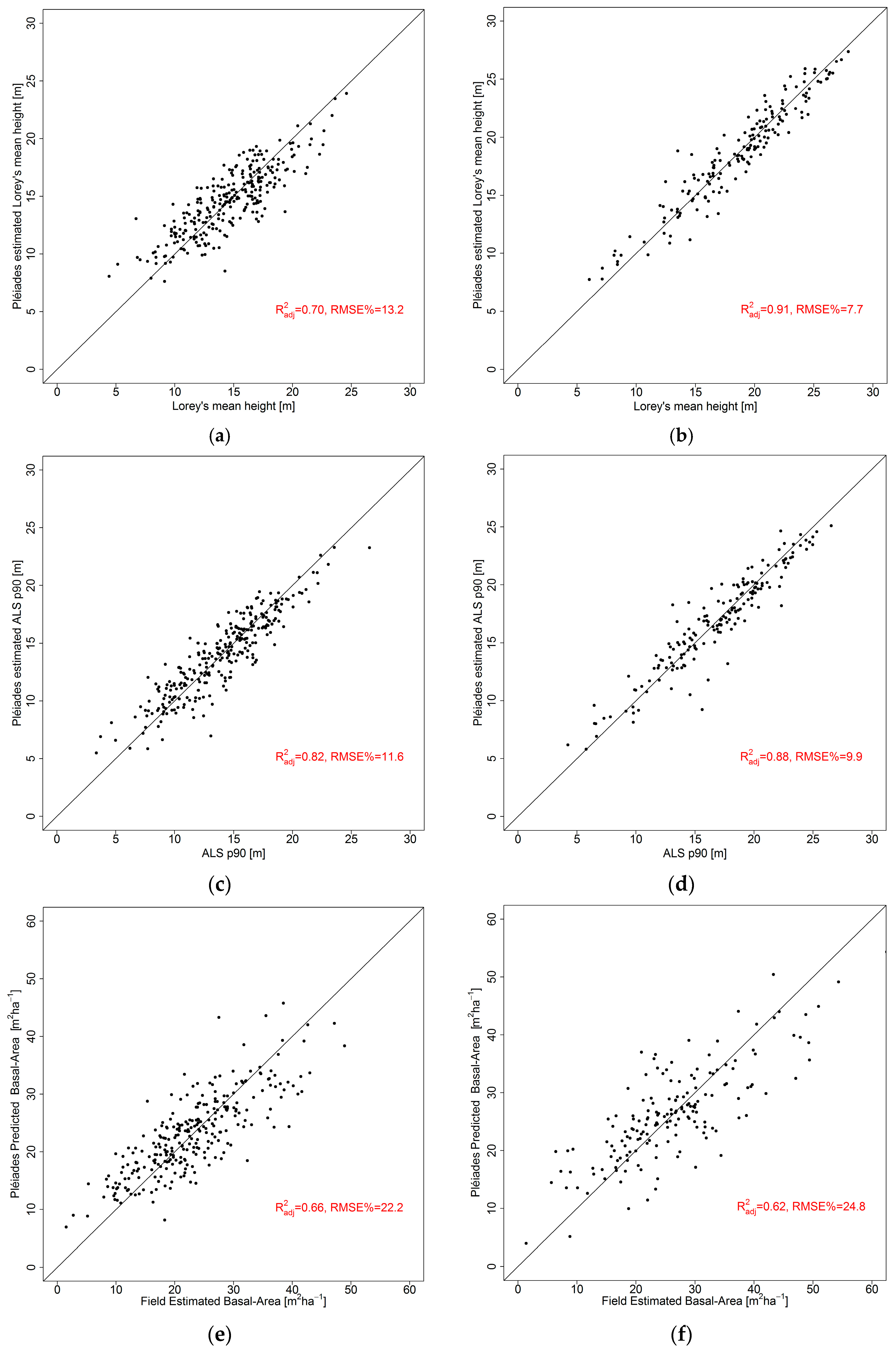
The image-matched height metrics showed a considerable potential for estimation of the target variables and, by adding also spectral derivatives and textural metrics, most models could be improved further. The tree height H_L was almost entirely described by the height metrics and the RMSE decreased only from 2.03 m to 1.92 m in Krycklan, and 1.62 m to 1.44 m in Remningstorp (Table 6 and Table 7). Similarly, the ALS p90 decreased from 1.68 m to 1.62 m in Krycklan, while no improvement could be achieved in Remningstorp (Table 6 and Table 7). This indicates that if only tree heights are of interest, there is a limited reimbursement of also acquiring and processing spectral and textural data. The accuracy of the height metrics modelled from Pléiades data are lower than models based solely on ALS data in Krycklan. However, the H_L was estimated better from VHR data (1.44 m) as from ALS data (1.60 m) in Remningstorp (Table 7 and Table 8). The accuracy of the height-modelled metrics is similar or slightly better than past studies based on other VHR sensors. When image-matched heights from the Ikonos sensor were used, the dominant forest height was estimated with 1.7 m RMSE [16], and when models based purely on spectral/textural features were used, Shamsoddini et al. [19] estimated the tree height with 1.9 m RMSE using WorldView-2 imagery; correspondingly, Kayitakire et al. [15] estimated the top height with 2.2 m, using Ikonos imagery. However, it is interesting that the latter two received such low RMSE values from models based merely on spectral/textural features. The pine plantation used as field data by Shamsoddini et al. [19] might have increased the textural importance, as the forest is similarly managed. This hypothesis is strengthened by the results from Kayitakire et al. [15], whose test site almost entirely consisted of a well-managed spruce plantation. This, therefore, would possibly explain the slightly larger improvement of height estimations in Remningtorp compared to Krycklan when the spectral/textural features were added (0.24 m and 0.12 m for H_L respectively), as Remningstorp is highly managed and Krycklan to a lower degree contains homogenous forest. A similar theory was also presented by Maack et al. [22], who claimed that natural regenerated forest would be more homogenous and therefore more sensible to textural metrics and less dependent on species, compared to other forests. Yu et al. [7] found that H_L could be estimated with 1.4 m RMSE in a Finnish boreal forest with approximately 75% coniferous forest. However, they used squared sample plots with 32 m × 32 m size, which gives a considerably larger plot area then in the current study (0.1 ha vs. 0.03 ha).

The estimation of BA was highly dependent on the height metrics, and the spectral/textural features added a limited improvement (0.5 to 0.8 m²·ha⁻¹; Table 6 and Table 7). The mean height was a suitable estimator for BA in Krycklan, and in Remningstorp the squared mean height was better suited. This could be due to different forest management actions, as thinning operations produce stands with different characteristics with respect to H_L, but similar characteristics for BA. Remningstorp is a highly managed test site, while Krycklan follows traditional management. Nevertheless, BA is frequently used to decide on forest management. The ALS-based models could to a slightly higher degree describe the BA well (4.3 m²·ha⁻¹ and 5.7 m²·ha⁻¹; Table 8). This might be due to the higher degree of penetration from ALS compared to the optical wavelengths in VHR data. The Pléiades-based models estimating BA achieved the lowest accuracy of the different target features, with RMSEs of 5.1 m²·ha⁻¹ (22%) and 6.6 m²·ha⁻¹ (25%), respectively. This is slightly better than Shamsoddini et al. [19] and St-Onge et al. [16], who reported the BA in a pine plantation at 7.7 m²·ha⁻¹ (23%) and 7.1 m²·ha⁻¹ (16%), respectively. However, it is higher both in absolute and relative terms compared to Yu et al. [7], who reported the BA with 4.3 m²·ha⁻¹ (16%), and Ozdemir and Karnieli [17], who reported the BA with 1.8 m²·ha⁻¹ (17%). The main difference and possible explanation of this are the larger plots (~0.1 ha) that were used in the two latter studies. Yu et al. [7] did also evaluate the effect of plot size, and could show that their estimations of BA increased by 3 to 10 percentage points when the plot size decreased from 32 m × 32 m to 16 m × 16 m. Consequently the present results seem to be of similar magnitude and reasonably accurate. The BA is overall estimated with comparable accuracy to VOL or AGB, regardless of sensor for both our test sites, and this is also the case in the study by Yu et al. [7].

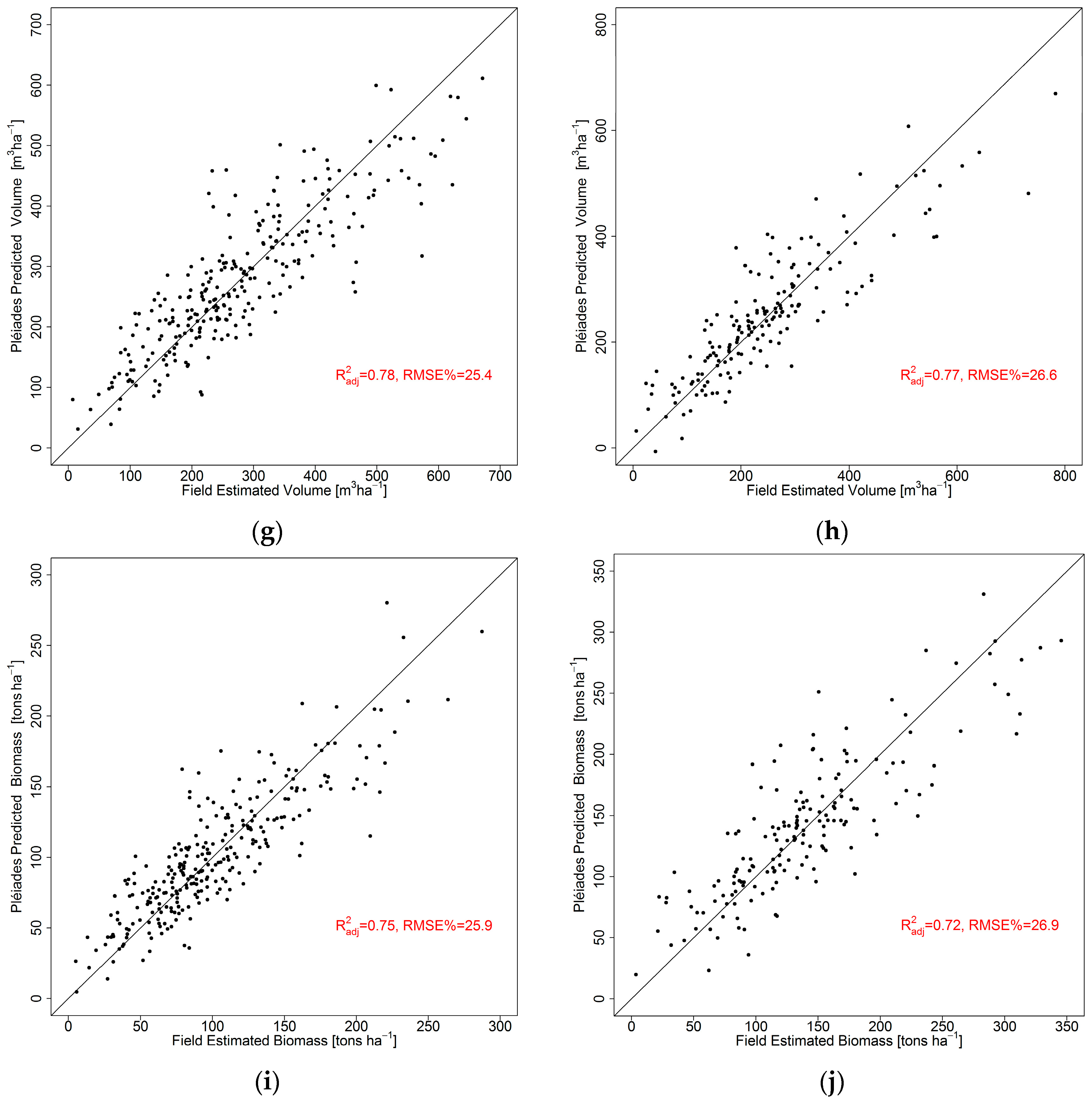
The VOL and AGB are highly correlated, as was reflected in the results. The R² values were between 0.73 and 0.77, and the RMSEs were 25.4% to 26.9% for both test sites and both attributes. From the scatter plots it can be concluded that estimations at higher volume/biomass possess considerably higher standard deviations, which might indicate a limited applicability for denser forest and southern forests with higher volumes/biomasses. Experience from using field data from these test sites together with other sensors (for example TanDEM-X radar data [36]) has shown that the standard deviations can remain constant along the entire evaluated range. In the current study, the heights generally had to be transformed to achieve significance in the regression modelling, and in Krycklan the heights were raised to the power of 2.3 while at Remningstorp the height was raised to the power of 2.6 and 2.7 for VOL and AGB, respectively (Table 6 and Table 7). In most VOL/AGB models, a non-transformed height variable complemented the transformed one to constitute the best model. The results are similar to what St-Onge et al. [16] achieved from Ikonos data (71 tons·ha⁻¹) and lower than Shamsoddini et al. [19] estimated from WorldView-2 spectral/textural features (90 m³·ha⁻¹, 30%). In relative terms, it is also lower than Ozdemir and Karnieli [17], who reported 44% RMSE (27 m³·ha⁻¹) for VOL, based on WorldView-2 imagery of an Israeli pine plantation forest. Immitzer et al. [21] estimated the VOL with 120 m³·ha⁻¹ (32%) from WorldView-2 data in a German forest. Moreover, Maack et al. [22] used Pléiades data to estimate AGB at a test site in Chile, and achieved 59 tons·ha⁻¹ (36%). Considering the results from other studies, the VHR data might be better suited for estimation of VOL/AGB in boreal forest than other forest types. Moreover, the Pléiades data specifically appear slightly better suited for estimation of forest attributes, compared to other VHR sensors.

It seems that the spectral and textural features were of greater importance for BA/VOL/AGB estimation than for those of H_L/ALS p90. This might be due to the missing information about forest density from merely height metrics (the BA was estimated with intermediate accuracy, R² = 0.51 to 0.58, from height metrics; Table 6), and this would therefore confirm the hypothesis that spectral/textural features from VHR imagery can contribute as a predictor for forest density. This study also confirms the hypothesis presented by Immitzer et al. and Maack et al. [21,22], that height metrics are superior to spectral derivatives and textural metrics when estimation of forest attributes are considered. This study found the spectral derivatives to be of similar importance to textural metrics, when the textural features were computed from VHR imagery with 1-m resolution, using an 11 × 11 pixels moving window. Smaller window sizes did not improve the results in this study, which is contrary to the conclusions of Maack et al. [22]. They found the smallest window size of 3 × 3 pixels gave the best AGB estimates. This study further confirms the hypothesis that textural metrics have a greater importance for estimation of forest attributes in homogenous forests (for example, plantation forests and well-managed forests) compared to more heterogeneous ones [15,16,17,19,22].

The potential of using Pléiades data as a replacement for ALS data seems promising. Overall, models from both sensors perform in similar ranges, although the performance of the ALS-based models appears to be more repeatable across the test sites. Nevertheless, the Pléiades-based models surpassed the performance of ALS-based models regarding H_L, VOL, and AGB in Remningstorp. A deeper understanding of the influence of the local forest conditions on the estimation results could increase the robustness and thus likelihood of replacing ALS data with Pléiades data.

Some of the past studies have involved some bias [7,22]. However, these have been based on non-parametric models (i.e., random forest or nearest-neighbour methods) and therefore this problem can be ignored in this study, which is based on regression analysis. The experience from the current study is that image matching from Pléiades imagery performs equally well as image matching with other VHR sensors (such as WorldView-2). 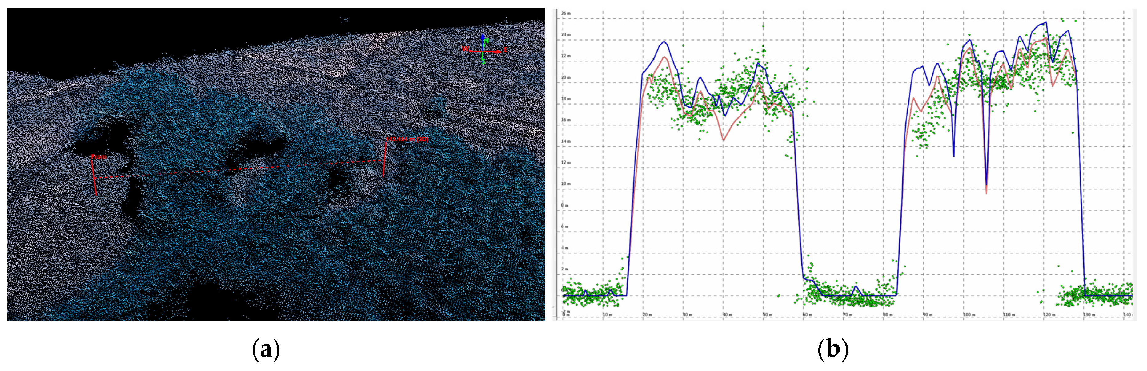Similarly to the Finnish study [7], it was found that the top height percentiles generally were most important, even though the mean height frequently became significant as an explanatory variable. In the current study, the ALS p90 was used as a height metric that is easy to obtain and practical for comparisons across test sites. It was also the ALS height metric that had the highest correlation to the image-matched height metrics. Sparse and low forest, typically young forest, was strongly influenced by underestimation in the image matching. Similarly, forest plots containing glades were frequently assigned too-low heights. This is likely due to the few (even absence of) matching points. Plots with deciduous trees in leaf-off conditions were also frequently noticed as outliers, probably by similar reasons. In this study, there was no obvious saturation in the estimations of VOL or AGB. However, the absence of a saturation effect could not be confirmed either, as the estimations of VOL/AGB exceeding ~250 tons·ha⁻¹ or 500 m³·ha⁻¹ started to flutter dubiously. In this study, most images possessed along-track incidence angles of about ±13° and, additionally, one more nadir acquisition. This causes the along-track intersection angles to be about optimum according to past studies, regarding the reconstruction of stereo heights [10,37]. However, the nadir image from Krycklan was −8°, which is less optimal than about 0°, as it causes one image pair to have a difference of only 5°, while the next stereo pair has a difference of ca. 20°. This causes the overall tri-stereo setup for Krycklan to be less optimal than the tri-stereo setup for Remningstorp. However, it is difficult to evaluate its influence on the final reconstructed heights, as other differences also separate the test sites.

5. Conclusions

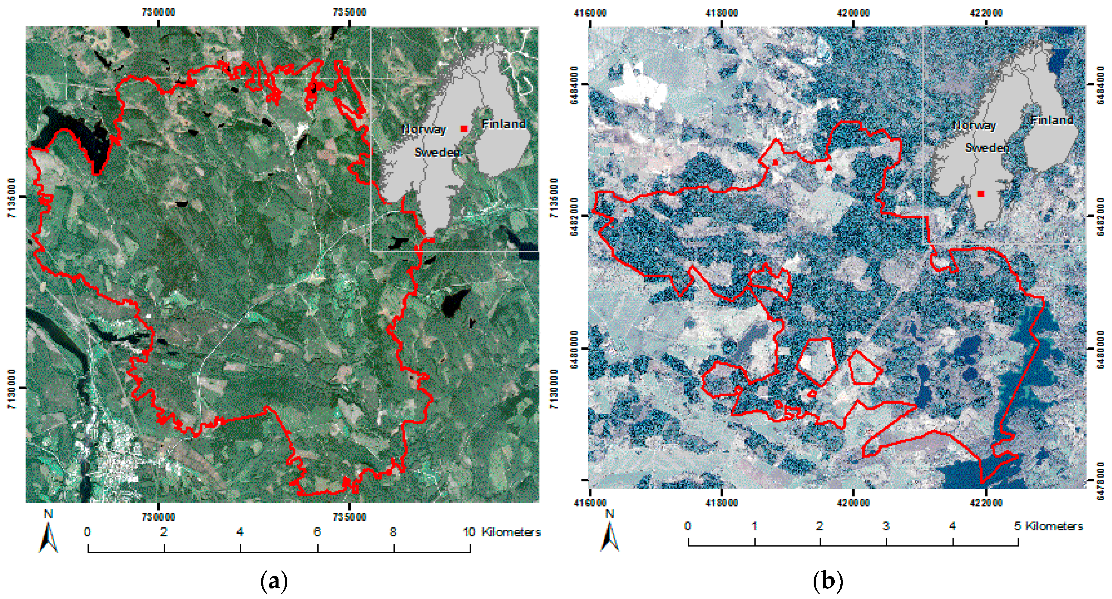
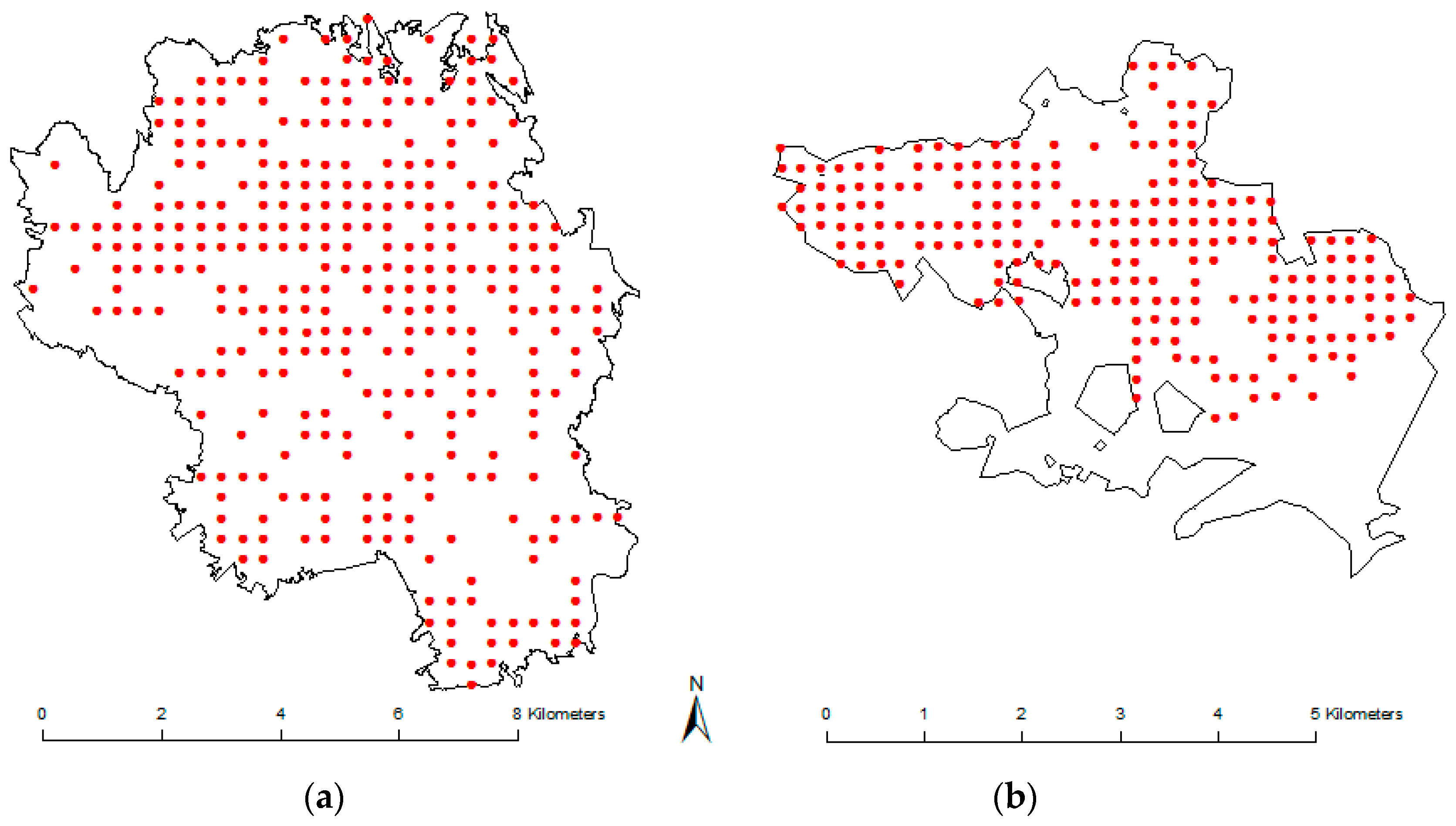
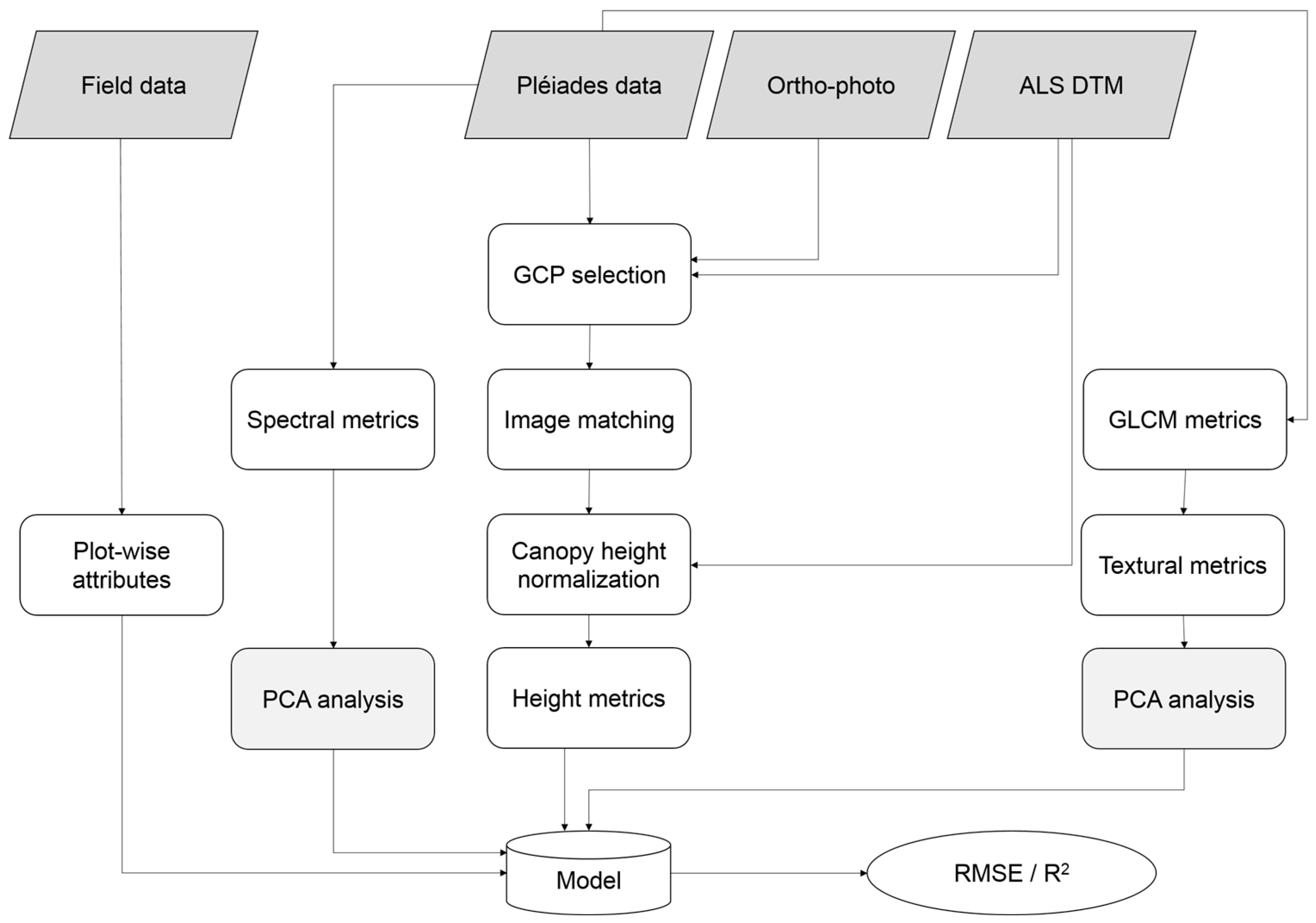
In this study, the potential of using very high resolution Pléiades imagery to estimate a number of common forest attributes in boreal forest was examined, when a high-resolution digital terrain model was available. The estimated attributes were H_L, ALS p90, BA, VOL, and AGB, derived for 10-m plots. The explanatory variables were derived from three processing alternatives. Height metrics were extracted from image matching of the images acquired from different incidence angles. Spectral derivatives were derived by performing principal component analysis of the spectral bands. Lastly, second-order textural metrics were extracted from a grey-level co-occurrence matrix, computed with an 11 × 11 pixels moving window. Principal component analysis was used to optimize the textural usage also. The analysis took place at two Swedish test sites, Krycklan and Remningstorp, containing boreal and hemi-boreal forest. It was found that the image-matched height metrics were most important in all models, and that the spectral and textural metrics contained similar information. Nevertheless, the best estimations were obtained when all three explanatory sources were used. The lowest RMSE was estimated with 1.4 m (7.7%) for H_L, 1.7 m (10%) for ALS p90, 5.1 m²·ha⁻¹ (22%) for BA, 66 m³·ha⁻¹ (27%) for VOL, and 26 tons·ha⁻¹ (26%) for AGB, respectively. For comparison, the same forest attributes were also estimated from ALS data. Overall, the Pléiades-based models showed similar performance to the ALS-based models, and for some attributes (H_L, VOL, and AGB) the Pléiades performance was even higher. The Pléiades results were similar across the test sites, despite the slightly different forest types and managements. Both test sites contained mainly coniferous forest and hence no influence of species was assessed. Sparse and low forest were generally assigned too-low heights in the image matching, and very dense forest with high volume/biomass were generally estimated with larger inaccuracy, which, however, could not directly be obtained as saturation. Textural features can improve the estimations, especially in homogenous forest, and a larger moving window (11 × 11 pixels) was preferred over smaller ones, though the computational cost is substantial.

In summary, this paper has shown the potential of using VHR satellite images suitable for image matching for the estimation of numerous relevant forest attributes. The presented method was shown to be an attractive alternative to ALS, and this method has the potential of being repeated frequently at reasonable cost.