
Agricultural Soil Alkalinity and Salinity Modeling in the Cropping Season in a Spectral Endmember Space of TM in Temperate Drylands, Minqin, China


Abstract
:
1. Introduction
2. Materials and Methods
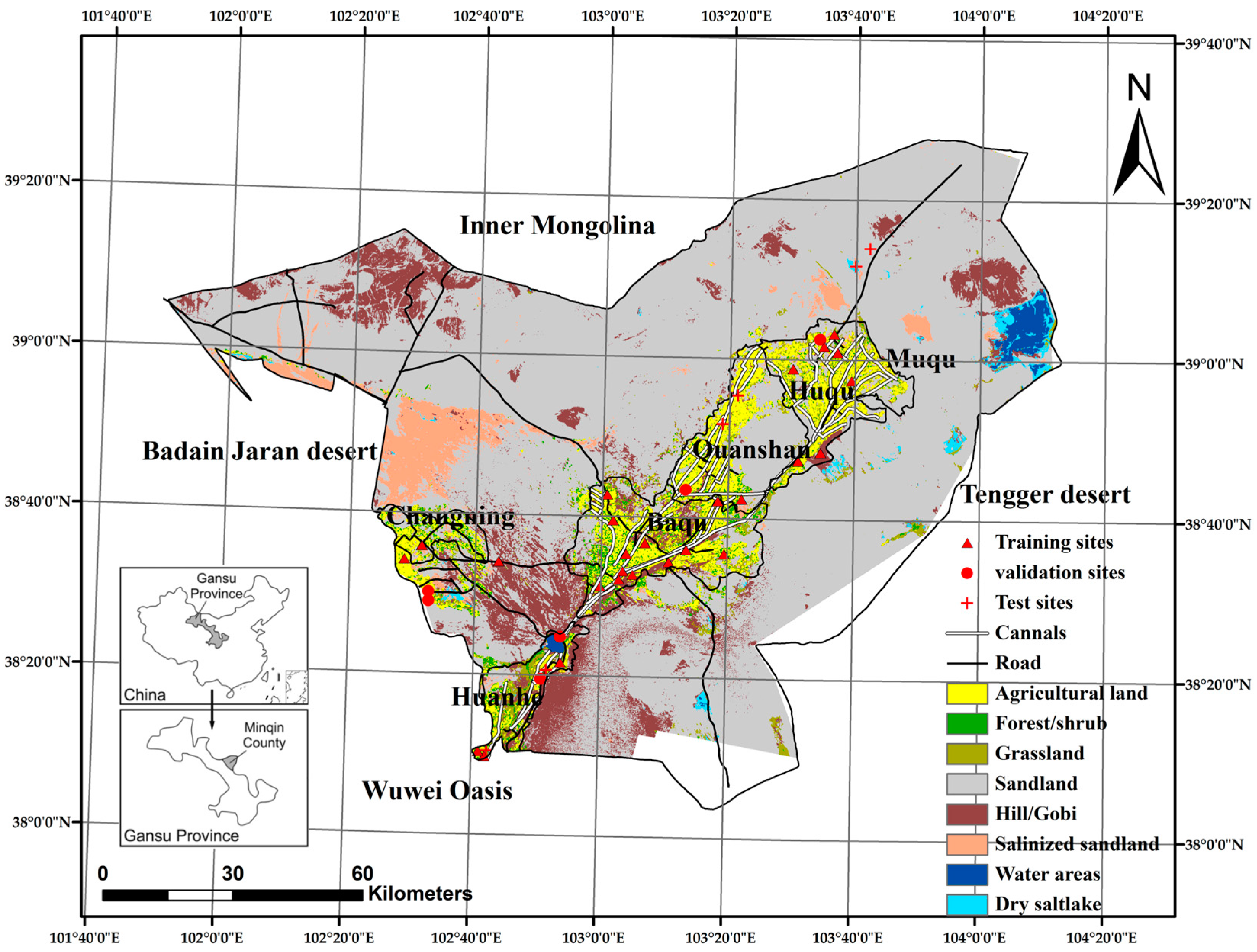
2.1. Study Area and in Situ Measurements
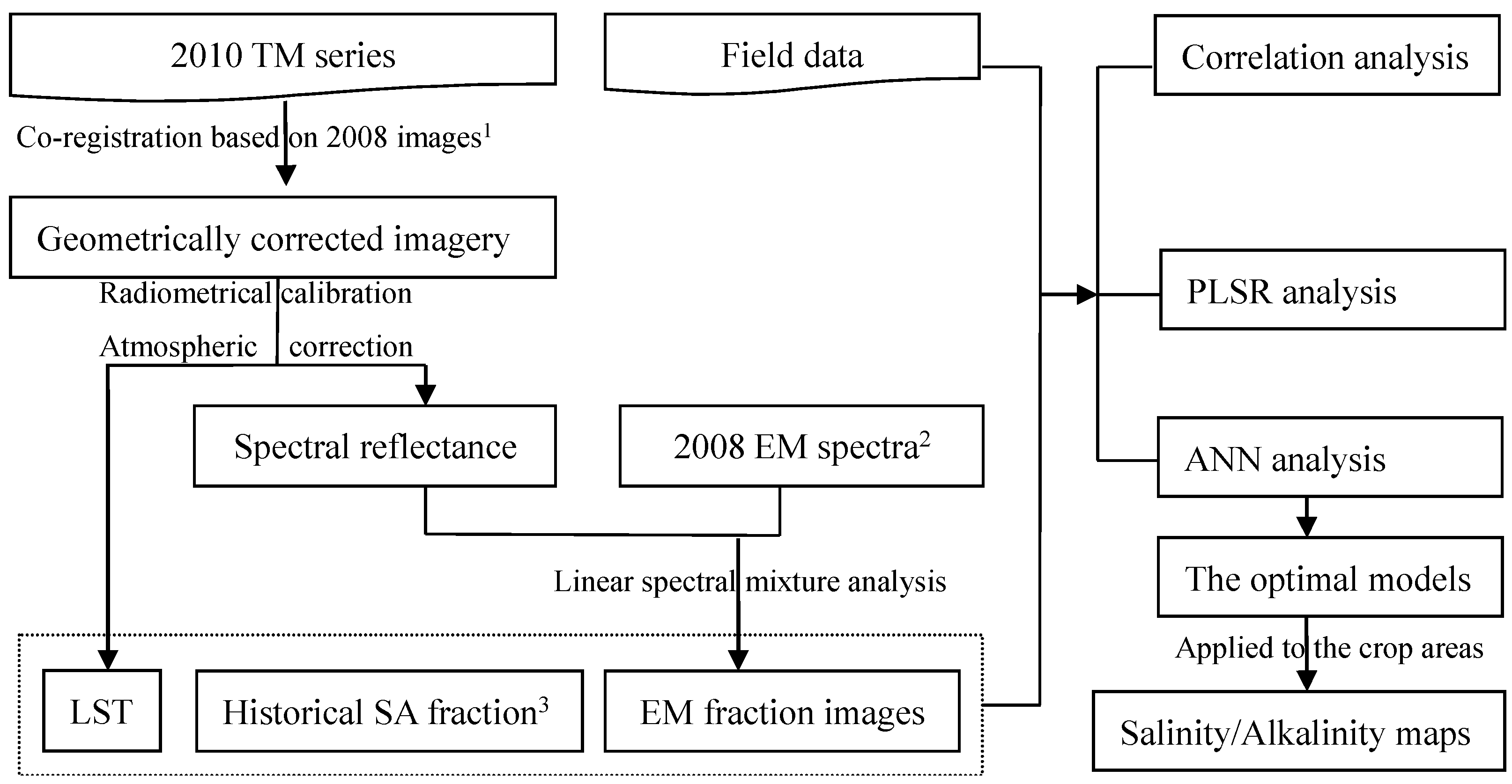
2.2. Remote Sensing Data and Preprocessing
2.3. SVD and LST for Solute Transport Process
2.4. PLSR and ANN Parameters and Calculation
3. Results
3.1. The Basic Description of Independent and Dependent Variables in the Study Area
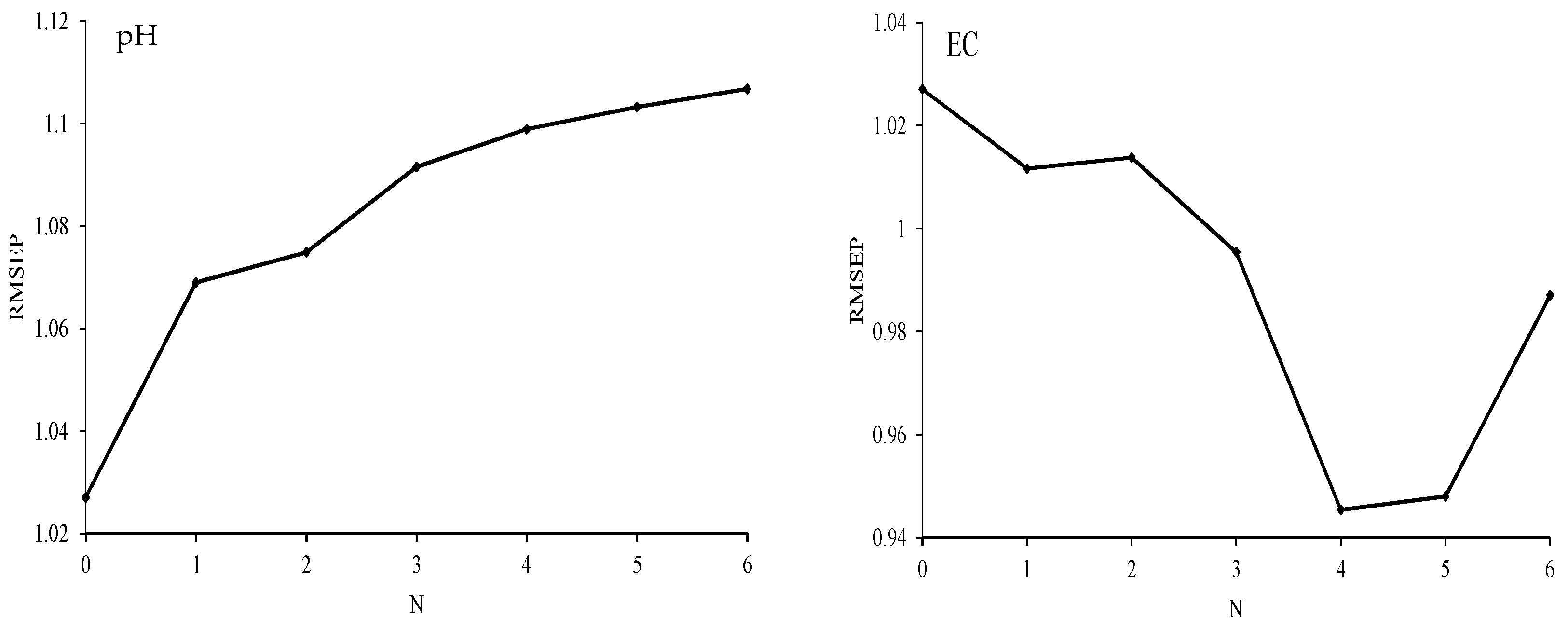
3.2. PLSR Models for Soil Salinity and Alkalinity Estimation
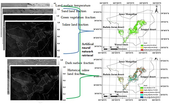
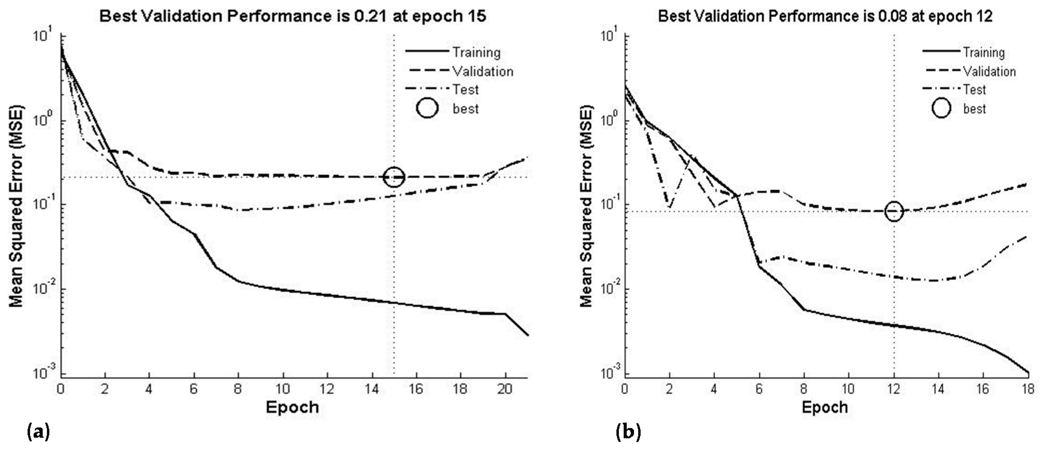
3.3. Neural Network Models for Salinity and Alkalinity Estimation
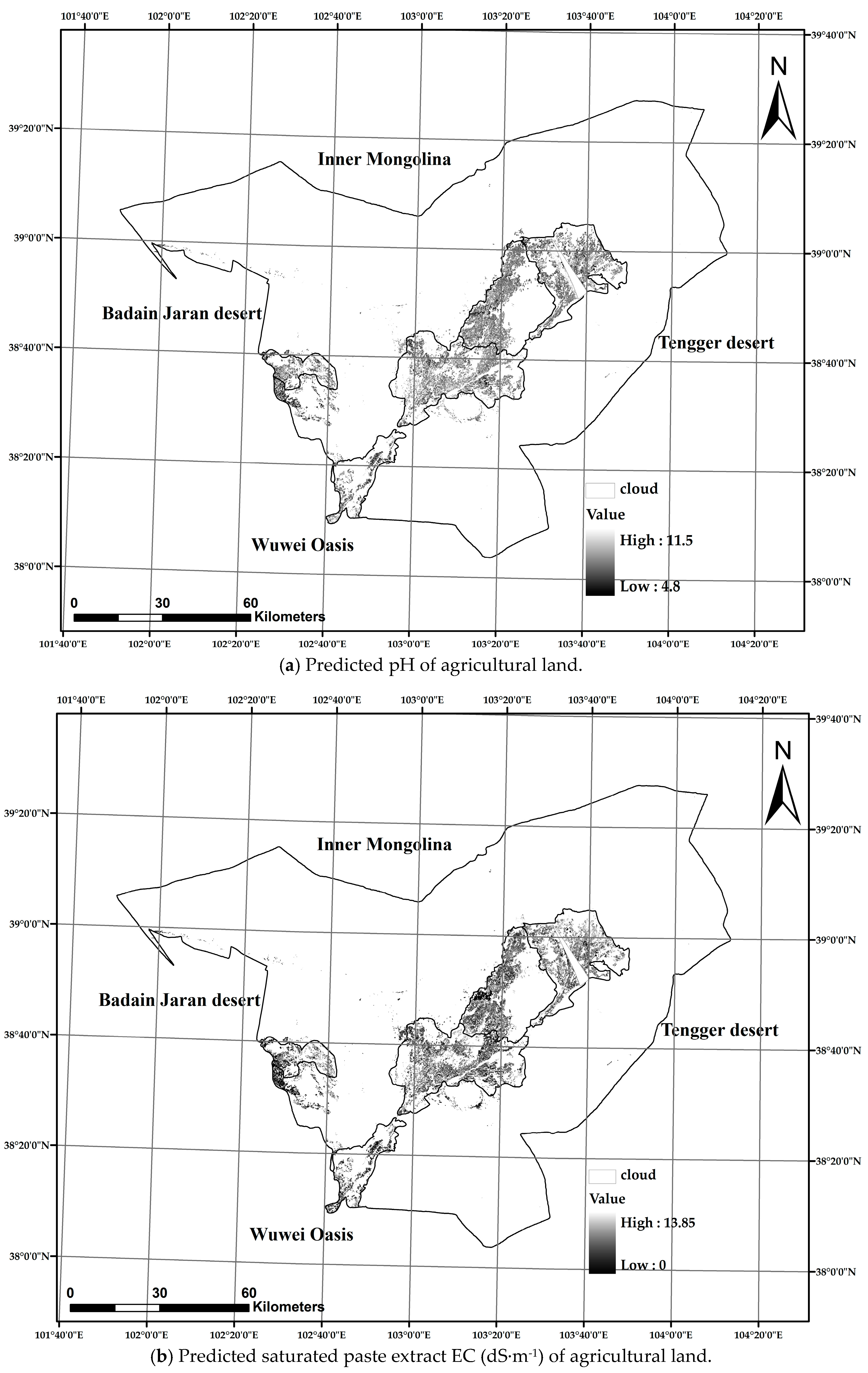
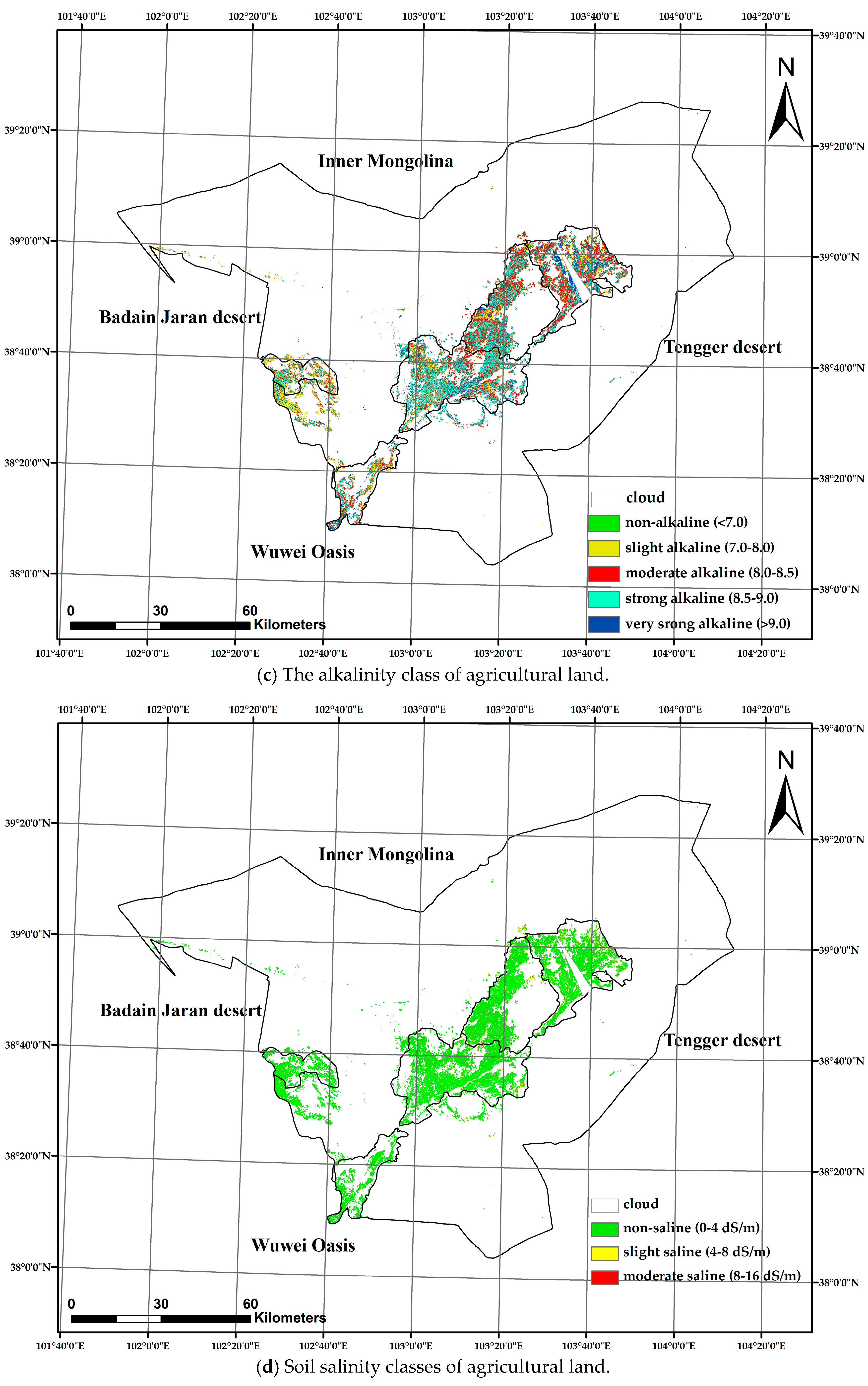
3.4. Soil Alkalinity and Salinity Mapping and Classification
4. Discussion
4.1. Agricultural Soil Alkalinity and Salinity Modeling in the Study Area
4.2. Potential of TM SVD for Regional Agricultural Soil Salinity and Alkalinity Mapping in the Root Zone
5. Conclusions
Acknowledgments
Author Contributions
Conflicts of Interest
References
- Farifteh, J.; Farshad, A.; George, R.J. Assessing salt-affected soils using remote sensing, solute modeling, and geophysics. Geoderma 2006, 130, 191–206. [Google Scholar] [CrossRef]
- Kassas, M. Seven paths to desertification. Desertification Control Bull. 1987, 15, 24–26. [Google Scholar]
- King, C.; Thomas, D.S. Monitoring environmental change and degradation in the irrigated oases of the Northern Sahara. J. Arid Environ. 2014, 103, 36–45. [Google Scholar] [CrossRef]
- Allbed, A.; Kumar, L.; Sinha, P. Mapping and modeling spatial variation in soil salinity in the Al Hassa Oasis based on remote sensing indicators and regression techniques. Remote Sens. 2014, 6, 1137–1157. [Google Scholar] [CrossRef]
- Fan, X.W.; Liu, Y.B.; Tao, J.M.; Weng, Y.L. Soil salinity retrieval from advanced multi-spectral sensor with partial least square regression. Remote Sens. 2015, 7, 488–511. [Google Scholar] [CrossRef]
- Zhang, W.T.; Wu, H.Q.; Gu, H.B.; Feng, G.L.; Wang, Z.; Sheng, J.D. Variability of soil salinity at multiple spatio-temporal scales and the related driving factors in the oasis areas of Xinjiang, China. Pedosphere 2014, 24, 753–762. [Google Scholar] [CrossRef]
- Tanji, K.K.; Kielen, N.C. Agricultural drainage water management in arid and semi-arid areas. In FAO Irrigation and Drainage; Food and Agriculture Organization of the United Nations: Rome, Italy, 2002; p. 61. [Google Scholar]
- Flowers, T.J.; Colmer, T.D. Salinity tolerance in halophytes. New Phytol. 2008, 179, 945–963. [Google Scholar] [CrossRef] [PubMed]
- Bai, L.; Wang, C.Z.; Zang, S.Y.; Zhang, Y.H.; Hao, Q.N.; Wu, Y.X. Remote sensing of soil alkalinity and salinity in the Wuyu’er-Shuangyang River Basin, Northeast China. Remote Sens. 2016. [Google Scholar] [CrossRef]
- Scudiero, E.; Skaggs, T.H.; Corwin, D.L. Regional-scale soil salinity assessment using Landsat ETM+ canopy reflectance. Remote Sens. Environ. 2015, 169, 335–343. [Google Scholar] [CrossRef]
- Sidike, A.; Zhao, S.; Wen, Y. Estimating soil salinity in Pingluo County of China using QuickBird data and soil reflectance spectra. Int. J. Appl. Earth Obs. Geoinf. 2014, 26, 156–175. [Google Scholar] [CrossRef]
- Dwivedi, R.S.; Rao, B.R.M. The selection of the best possible Landsat TM band combination for delineating salt-affected soils. Int. J. Remote Sens. 1992, 13, 2051–2058. [Google Scholar] [CrossRef]
- Fernandez-Buces, N.; Siebe, C.; Cram, S.; Palacio, J.L. Mapping soil salinity using a combined spectral response index for bare soil and vegetation: A case study in the former Lake Texcoco, Mexico. J. Arid Environ. 2006, 65, 644–667. [Google Scholar] [CrossRef]
- Wu, W.; Mhaimeed, A.S.; Al-Shafie, W.M.; Ziadat, F.; Dhehibi, B.; Nangia, V.; de Pauw, E. Mapping soil salinity changes using remote sensing in Central Iraq. Geod. Reg. 2004, 2, 21–31. [Google Scholar] [CrossRef]
- Fan, X.; Pedroli, B.; Liu, G.; Liu, Q.; Liu, H.; Shu, L. Soil salinity development in the yellow river delta in relation to groundwater dynamics. Land Degrad. Dev. 2002, 23, 175–189. [Google Scholar] [CrossRef]
- Fan, X.; Weng, Y.; Tao, J. Towards decadal soil salinity mapping using Landsat time series data. Int. J. Appl. Earth Obs. Geoinf. 2006, 52, 32–41. [Google Scholar] [CrossRef]
- Akramkhanov, A.; Vlek, P.L.J. The assessment of spatial distribution of soil salinity risk using neural network. Environ. Monit. Assess. 2012, 184, 2475–2485. [Google Scholar] [CrossRef] [PubMed]
- Samuel-Rosa, A.; Heuvelink, G.; Vasques, G.; Anjos, L. Do more detailed environmental covariates deliver more accurate soil maps? Geoderma 2015, 243, 214–227. [Google Scholar] [CrossRef]
- Small, C. The Landsat ETM+ spectral mixing space. Remote Sens. Environ. 2004, 93, 1–17. [Google Scholar] [CrossRef]
- Small, C.; Milesi, C. Multi-scale standardized spectral mixture models. Remote Sens. Environ. 2013, 136, 442–454. [Google Scholar] [CrossRef]
- Sun, D.; Liu, N. Coupling spectral unmixing and multiseasonal remote sensing for temperate dryland land-use/land-cover mapping in Minqin County, China. Int. J. Remote Sens. 2015, 36, 3636–3658. [Google Scholar] [CrossRef]
- Sun, D. Detection of dryland degradation using Landsat spectral unmixing remote sensing with syndrome concept in Minqin County, China. Int. J. Appl. Earth Obs. Geoinf. 2015, 41, 34–45. [Google Scholar] [CrossRef]
- Asner, G.P.; Bateson, C.A.; Privette, J.L.; Elsaleous, N.; Wessman, C.A. Estimating vegetation structural effects on carbon uptake using satellite data fusion and inverse modeling. J. Geophys. Res. 1998, 103, 28839–28853. [Google Scholar] [CrossRef]
- Hall, F.G.; Shimabukuro, Y.E.; Huemmerich, K.F. remote sensing of forest biophysical structure using mixture decomposition and geometric reflectance models. Ecol. Appl. 1995, 5, 993–1013. [Google Scholar] [CrossRef]
- Sonnentag, O.; Chen, J.M.; Roberts, D.A.; Talbot, J.; Halligan, K.Q.; Govind, A. Mapping tree and shrub leaf area indices in an ombrotrophic peatland through multiple endmember spectral unmixing. Remote Sens. Environ. 2007, 109, 342–360. [Google Scholar] [CrossRef]
- Farifteh, J.; van der Meer, F.; Atzberger, C.; Carranza, E. Quantitative analysis of salt-affected soil reflectance spectra: A comparison of two adaptive methods (PLSR and ANN). Remote Sens. Environ. 2007, 110, 59–78. [Google Scholar] [CrossRef]
- Lek, S.; Guégan, J.F. Artificial neural networks as a tool in ecological modeling, an introduction. Ecol. Model. 1999, 120, 65–73. [Google Scholar] [CrossRef]
- Dixon, B.; Candade, N. Multispectral land use classification using neural networks and support vector machines: One or the other, or both? Int. J. Remote Sens. 2008, 29, 1185–1206. [Google Scholar] [CrossRef]
- Gansu Provincial Water Resources Department; Gansu Provincial Development and Reform Commission. Planning of Key Rehabilitation and Comprehensive Management for Shiyang River Basin; Gansu Provincial Water Resources Department; Gansu Provincial Development and Reform Commission: Lanzhou, China, 2007. (In Chinese)
- Sun, D.; Dawson, R.; Li, H.; Li, B. Modeling desertification change in Minqin county, China. Environ. Monit. Assess. 2005, 108, 169–188. [Google Scholar] [CrossRef] [PubMed]
- ISSCAS (Institute of Soil Sciences Chinese Academy of Sciences). Physical and Chemical Analysis Methods of Soils; Shanghai Science Technology Press: Shanghai, China, 1978. (In Chinese) [Google Scholar]
- Wu, C.; Murray, A.T. Estimating impervious surface distribution by spectral mixture analysis. Remote Sens. Environ. 2003, 84, 493–505. [Google Scholar] [CrossRef]
- Landsat Project Science Office. Landsat 7 Science Data Users Handbook. Goddard Space Flight Center. Available online: http://landsat.gsfc.nasa.gov/?p=12723 (accessed on 26 June 2015).
- Markham, B.L.; Barker, J.L. Landsat MSS and TM postcalibration dynamic ranges, exoatmospheric reflectances and at-satellite temperatures. EOSAT Landsat Tech. Notes 1986, 1, 3–8. [Google Scholar]
- Wukelic, G.E.; Gibbons, D.E.; Martucci, L.M.; Foote, H.P. Radiometric calibration of Landsat Thematic Mapper thermal band. Remote Sens. Environ. 1989, 28, 339–347. [Google Scholar] [CrossRef]
- Washburne, J.C. A Distributed Surface Temperature and Energy Balance Model of a Semi-Arid Watershed. Ph.D. Thesis, University of Arizona, Tucson, AZ, USA, 1994. [Google Scholar]
- Jiménez Muñoz, J.C.; Sobrino, J.A. A generalized single-channel method for retrieving land surface temperature from remote sensing data. J. Geophys. Res. 2003. [Google Scholar] [CrossRef]
- Sobrino, J.A.; Jiménez-Muñoz, J.C.; Paolini, L. Land surface temperature retrieval from LANDSAT TM 5. Remote Sens. Environ. 2004, 90, 434–440. [Google Scholar] [CrossRef]
- Yu, Y.; Gu, H.B.; Zhang, L.; Yan, A.; Sheng, J.D.; Chai, Q.; Xie, F.H.; Cai, Y.F. Analysis of soil salt characteristics in oasis farmland. J China Agric. Univ. 2016, 21, 89–95. (In Chinese) [Google Scholar]
- Yu, Y.P. Soil alkalinity and its prevention. Soils 1984, 5, 163–170. (In Chinese) [Google Scholar]
- Bernstein, L. Effects of salinity and sodicity on plant growth. Annu. Rev. Phytopathol. 1975, 13, 295–312. [Google Scholar] [CrossRef]
- Huang, P.M.; Li, Y.; Sumner, M.E. Soil Sciences: Resource Management and Environmental Impacts; CRC Press: Boca Raton, FL, USA, 2012. [Google Scholar]
- Hornik, K.; Stinchcombe, M.; White, H. Multilayer feedforward networks are universal approximators. Neural Netw. 1989, 2, 359–366. [Google Scholar] [CrossRef]
- Dawson, C.W.; Wilby, R.L. Hydrological modeling using artificial neural networks. Prog. Phys. Geogr. 2001, 25, 80–108. [Google Scholar] [CrossRef]
- Schultz, A.; Wieland, R.; Lutze, G. Neural networks in agroecological modeling—Stylish application or helpful tool? Comput. Electron. Agric. 2000, 29, 73–97. [Google Scholar] [CrossRef]
- Haykin, S. Neural Networks: A Comprehensive Foundation, 2nd ed.; Prentice–Hall Inc.: Upper Saddle River, NJ, USA, 1999. [Google Scholar]
- Fletcher, D.; Goss, E. Forecasting with neural networks: An application using bankruptcy data. Inf. Manag. 1993, 24, 159–167. [Google Scholar] [CrossRef]
- Richards, L.A. Diagnosis and Improvement of Saline and Alkali Soils; U.S. Department of Agriculture: Washington, DC, USA, 1954.
- Xin, J.F.; Zhang, G.Y.; Li, Y.Z. The different soil electrical conductivity types and their relations. In Movement of Water-Salts in Salinized Soils; Shi, Y.C., Ed.; Beijing Agricultural University Publishing: Beijing, China, 1985; pp. 151–158. [Google Scholar]
- Atzberger, C.; Darvishzadeh, R.; Immitzer, M.; Schlerf, M.; Skidmore, A.; Maire, G. Comparative analysis of different retrieval methods for mapping grassland leaf area index using airborne imaging spectroscopy. Int. J. Appl. Earth Obs. Geoinf. 2015, 43, 19–31. [Google Scholar] [CrossRef]


| Soil Variables | Subsets | Sample Number | Mean | Minimum | Maximum | Std. 1 |
|---|---|---|---|---|---|---|
| pH | training | 26 | 8.57 | 7.70 | 9.89 | 0.44 |
| validation | 6 | 8.36 | 7.07 | 9.16 | 0.76 | |
| test | 6 | 8.83 | 8.53 | 9.40 | 0.33 | |
| EC | training | 26 | 0.37 | 0.08 | 1.43 | 0.28 |
| validation | 6 | 0.40 | 0.15 | 1.15 | 0.38 | |
| test | 6 | 0.33 | 0.07 | 0.91 | 0.31 |
| Variables | Definition | Unit | Mean | Minimum | Maximum | Std. 1 |
|---|---|---|---|---|---|---|
| pH | Soil reaction | 8.58 | 7.07 | 9.89 | 0.49 | |
| EC | Soil electrical conductivity | dS·m −1 | 0.37 | 0.07 | 1.43 | 0.29 |
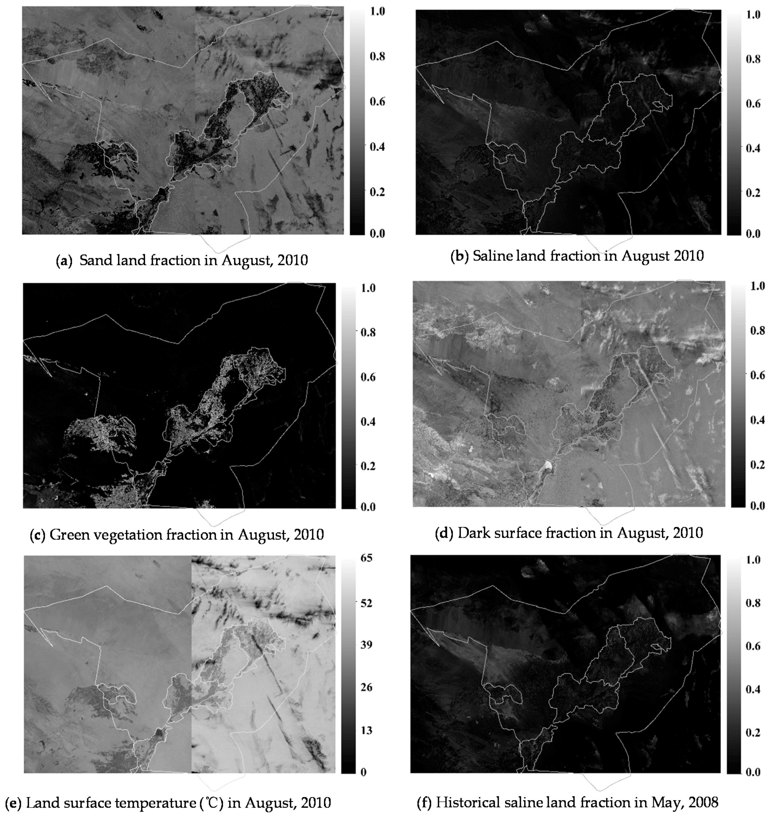
| SL | Sand land fraction | 0.19 | 0 | 0.52 | 0.15 | |
| SA | Saline land fraction | 0.09 | 0.01 | 0.2 | 0.04 | |
| GV | Green vegetation fraction | 0.29 | 0.01 | 0.81 | 0.23 | |
| DA | Dark surface fraction | 0.43 | 0.1 | 0.61 | 0.11 | |
| SAH | Historical saline land fraction in 2008 | 0.11 | 0.01 | 0.23 | 0.06 | |
| LST | Land surface temperature | °C | 36.13 | 25.02 | 51.87 | 7.55 |
| Variables | pH | EC | SL | SA | GV | DA | SAH | LST |
|---|---|---|---|---|---|---|---|---|
| pH | 1 | −0.569 *** | 0.217 | −0.002 | −0.137 | −0.013 | −0.304 * | 0.127 |
| EC | 1 | 0.123 | 0.147 | −0.129 | 0.044 | 0.313 * | 0.36 ** | |
| SL | 1 | 0.329 ** | −0.879 *** | 0.337 ** | 0.014 | 0.804 *** | ||
| SA | 1 | −0.435 *** | 0.08 | 0.38 ** | 0.252 | |||
| GV | 1 | −0.716 *** | 0.001 | −0.607 *** | ||||
| DA | 1 | −0.165 | 0.068 | |||||
| SAH | 1 | 0.005 | ||||||
| LST | 1 |
| N | Performances | Standardized Coefficients | ||||||||
|---|---|---|---|---|---|---|---|---|---|---|
| RPD | R2 | RMSE | SL | SA | GV | DA | SAH | LST | ||
| pH | 1 | 0.35 | 0.11 | 0.46 | 0.13 | 0 | −0.08 | −0.01 | −0.19 * | 0.08 |
| EC | 4 | 0.75 | 0.36 | 0.23 | −0.56 ** | 0.01 | 0.18 ** | 0.39 ** | 0.4 *** | 0.86 *** |
| pH | Predictor Variable Combinations | N | ||||||||
|---|---|---|---|---|---|---|---|---|---|---|
| 5 | 6 | 7 | 8 | 9 | 10 | 11 | 12 | 13 | ||
| R2 | ALL | 0.70 | 0.76 | 0.66 | 0.64 | 0.67 | 0.66 | 0.68 | 0.72 | 0.65 |
| ALL-SA | 0.70 | 0.66 | 0.60 | 0.63 | 0.60 | 0.57 | 0.64 | |||
| ALL-DA | 0.71 | 0.68 | 0.71 | 0.71 | 0.69 | 0.69 | 0.70 | |||
| ALL-LST | 0.61 | 0.61 | 0.60 | 0.68 | 0.68 | 0.60 | 0.60 | |||
| ALL-GV | 0.70 | 0.70 | 0.70 | 0.69 | 0.70 | 0.66 | 0.66 | |||
| ALL-SL | 0.65 | 0.70 | 0.67 | 0.69 | 0.69 | 0.66 | 0.66 | |||
| ALL-SAH | 0.71 | 0.73 | 0.66 | 0.70 | 0.67 | 0.60 | 0.68 | |||
| RMSE | ALL | 0.27 | 0.24 | 0.28 | 0.30 | 0.28 | 0.29 | 0.28 | 0.26 | 0.29 |
| ALL-SA | 0.28 | 0.29 | 0.32 | 0.30 | 0.31 | 0.32 | 0.30 | |||
| ALL-DA | 0.26 | 0.28 | 0.27 | 0.27 | 0.27 | 0.27 | 0.28 | |||
| ALL-LST | 0.31 | 0.31 | 0.32 | 0.29 | 0.28 | 0.31 | 0.33 | |||
| ALL-GV | 0.27 | 0.27 | 0.27 | 0.30 | 0.27 | 0.29 | 0.29 | |||
| ALL-SL | 0.32 | 0.27 | 0.28 | 0.27 | 0.27 | 0.29 | 0.28 | |||
| ALL-SAH | 0.26 | 0.26 | 0.29 | 0.30 | 0.30 | 0.33 | 0.28 | |||
| EC | Predictor Variable Combinations | N | |||||||||
|---|---|---|---|---|---|---|---|---|---|---|---|
| 4 | 5 | 6 | 7 | 8 | 9 | 10 | 11 | 12 | 13 | ||
| R2 | ALL | 0.64 | 0.63 | 0.65 | 0.65 | 0.64 | 0.61 | 0.64 | 0.65 | 0.66 | |
| ALL-SA | 0.62 | 0.67 | 0.66 | 0.61 | 0.66 | 0.61 | 0.66 | ||||
| ALL-GV | 0.67 | 0.67 | 0.67 | 0.66 | 0.69 | 0.66 | 0.66 | ||||
| ALL-DA | 0.69 | 0.72 | 0.64 | 0.66 | 0.71 | 0.67 | 0.74 | ||||
| ALL-SAH | 0.63 | 0.61 | 0.68 | 0.62 | 0.63 | 0.66 | 0.71 | ||||
| ALL-SL | 0.67 | 0.63 | 0.65 | 0.67 | 0.68 | 0.70 | 0.66 | ||||
| ALL-LST | 0.34 | 0.60 | 0.55 | 0.31 | 0.48 | 0.44 | 0.67 | ||||
| ALL-DA, SA | 0.61 | 0.67 | 0.66 | 0.68 | 0.64 | ||||||
| ALL-DA, GV | 0.68 | 0.72 | 0.73 | 0.70 | 0.69 | ||||||
| ALL-DA, SAH | 0.68 | 0.64 | 0.70 | 0.65 | 0.79 | ||||||
| ALL-DA, SL | 0.60 | 0.62 | 0.63 | 0.63 | 0.68 | ||||||
| ALL-DA, LST | 0.60 | 0.64 | 0.71 | 0.46 | 0.69 | ||||||
| ALL-DA, SAH, SA | 0.59 | 0.60 | 0.57 | 0.61 | |||||||
| ALL-DA, SAH, GV | 0.66 | 0.67 | 0.71 | 0.78 | |||||||
| ALL-DA, SAH, SL | 0.60 | 0.67 | 0.71 | 0.68 | |||||||
| ALL-DA, SAH, LST | 0.49 | 0.65 | 0.40 | 0.43 | |||||||
| RMSE | ALL | 0.18 | 0.18 | 0.17 | 0.19 | 0.18 | 0.18 | 0.18 | 0.17 | 0.17 | |
| ALL-SA | 0.18 | 0.18 | 0.17 | 0.18 | 0.17 | 0.18 | 0.17 | ||||
| ALL-GV | 0.17 | 0.17 | 0.17 | 0.17 | 0.16 | 0.17 | 0.17 | ||||
| ALL-DA | 0.17 | 0.15 | 0.19 | 0.17 | 0.16 | 0.18 | 0.15 | ||||
| ALL-SAH | 0.18 | 0.18 | 0.17 | 0.21 | 0.18 | 0.19 | 0.16 | ||||
| ALL-SL | 0.17 | 0.18 | 0.18 | 0.17 | 0.16 | 0.22 | 0.17 | ||||
| ALL-LST | 0.25 | 0.19 | 0.20 | 0.25 | 0.24 | 0.24 | 0.21 | ||||
| ALL-DA, SA | 0.18 | 0.17 | 0.17 | 0.17 | 0.18 | ||||||
| ALL-DA, GV | 0.17 | 0.15 | 0.16 | 0.16 | 0.17 | ||||||
| ALL-DA, SAH | 0.17 | 0.19 | 0.16 | 0.17 | 0.13 | ||||||
| ALL-DA, SL | 0.18 | 0.18 | 0.18 | 0.18 | 0.16 | ||||||
| ALL-DA, LST | 0.22 | 0.18 | 0.16 | 0.21 | 0.16 | ||||||
| ALL-DA, SAH, SA | 0.19 | 0.18 | 0.20 | 0.18 | |||||||
| ALL-DA, SAH, GV | 0.17 | 0.17 | 0.18 | 0.15 | |||||||
| ALL-DA, SAH, SL | 0.18 | 0.17 | 0.16 | 0.17 | |||||||
| ALL-DA, SAH, LST | 0.21 | 0.17 | 0.24 | 0.22 | |||||||
| Predictor Variable Combination | N | R2 | RMSE | Predictive Model Parameters | |||||||
|---|---|---|---|---|---|---|---|---|---|---|---|
| Tra. | Val. | Test | Tra. | Val. | Test | R2 | RMSE | RPD | |||
| pH | SL, SA, GV, DA, SAH, LST | 6 | 0.96 | 0.59 | 0.70 | 0.08 | 0.46 | 0.36 | 0.76 | 0.24 | 1.96 |
| EC | SL, SA, GV, LST | 9 | 0.95 | 0.33 | 0.84 | 0.06 | 0.29 | 0.12 | 0.79 | 0.13 | 1.95 |
| Non-Alkaline | Slight Alkaline | Moderate Alkaline | Strong Alkaline | Very Strong Alkaline | % Total Area | |
|---|---|---|---|---|---|---|
| Non-saline | 241.65 | 14,519.7 | 32,378.76 | 38,041.2 | 15,937.83 | 91.93 |
| Slight saline | 10.62 | 1730.43 | 4076.64 | 1432.26 | 738.54 | 7.27 |
| Moderate saline | 2.25 | 406.26 | 328.41 | 77.22 | 68.58 | 0.80 |
| % Total area | 0.23 | 15.14 | 33.44 | 35.96 | 15.22 |
© 2016 by the authors; licensee MDPI, Basel, Switzerland. This article is an open access article distributed under the terms and conditions of the Creative Commons Attribution (CC-BY) license (http://creativecommons.org/licenses/by/4.0/).
Share and Cite
Sun, D.; Jiang, W. Agricultural Soil Alkalinity and Salinity Modeling in the Cropping Season in a Spectral Endmember Space of TM in Temperate Drylands, Minqin, China. Remote Sens. 2016, 8, 714. https://doi.org/10.3390/rs8090714
Sun D, Jiang W. Agricultural Soil Alkalinity and Salinity Modeling in the Cropping Season in a Spectral Endmember Space of TM in Temperate Drylands, Minqin, China. Remote Sensing. 2016; 8(9):714. https://doi.org/10.3390/rs8090714
Chicago/Turabian StyleSun, Danfeng, and Wanbei Jiang. 2016. "Agricultural Soil Alkalinity and Salinity Modeling in the Cropping Season in a Spectral Endmember Space of TM in Temperate Drylands, Minqin, China" Remote Sensing 8, no. 9: 714. https://doi.org/10.3390/rs8090714
APA StyleSun, D., & Jiang, W. (2016). Agricultural Soil Alkalinity and Salinity Modeling in the Cropping Season in a Spectral Endmember Space of TM in Temperate Drylands, Minqin, China. Remote Sensing, 8(9), 714. https://doi.org/10.3390/rs8090714