1. Introduction
The assessment of the kinematical evolution of the slow landslides is challenging for the analysis and zonation of the risk in urban areas. Indeed, the capability to detect the spatial kinematical variability of a slow landslide processes can represent a fundamental source of knowledge to support the land management decision for the development of infrastructures in urban areas. In this perspective, the evaluation of the landslide displacement field at ground level in a certain time span, can impart important information for the prediction of the expected damage to buildings and infrastructure. In addition, the understanding of the landslides kinematics is also crucial in defining efficient prevention and mitigation strategies and can be effectively pursued only if multidisciplinary data, both in terms of temporal and spatial coverage of the area is available.
The kinematics of the landslide phenomena has been analyzed in a large number of scientific studies; the approaches range from the analytical one-dimensional (1D) infinite slope models, suitable for landslides bodies with sliding surface depth about constant and significantly lower than the landslide length [
1,
2,
3,
4,
5], to more sophisticated two- (2D) and three-dimensional (3D) Finite Element (FE) models aimed at detecting the different kinematical sectors along the slope area [
6,
7,
8,
9]. In particular, the recent development of three-dimensional numerical codes allows us to carry out simulations of the displacement rate field of a landslide process in a more realistic and accurate way. The simulations of the landslide kinematics are achieved through the implementation in a numerical domain, of the available a-priori information on the slope, as the topography, the landslide body geometry and the mechanical properties of the involved geomaterials. Such enhanced information is retrieved through a significant increase of the computational load of the 3D models with respect to 2D models. However, this computational complexity can be correctly reduced when the examined landslide shows the typical kinematical features of a landslide creep, i.e., landslide phenomena are characterized by very low pore water pressure variation rates and consequently, the displacement rates do not significantly change with time.
The reliability of the performed numerical models significantly improves when the same models are calibrated and validated by using the measurements collected by means of the available monitoring networks. To this purpose, the inverse analysis carried out via optimization procedures aimed at searching for the model best-fitting solution against the monitoring dataset, represents a very efficient tool in identifying the physical process that governs the observed phenomenon [
8,
9]. To accomplish an effective inverse analysis of a 3D landslide model, spatially distributed surface measurements are needed. In particular, a network of displacement measure points that covers a large portion of the landslide body is required to correctly constrain the three-dimensional FE model. However, surface deformation measurements based on in situ research (inclinometers, GPS, leveling) are often unavailable, or only partially available, due to the high costs related to these technologies, especially if needed for long-term research. In this context, satellite techniques offer an effective and reliable alternative or a complementary tool to traditional in situ research. In particular, the Differential Synthetic Aperture Radar (SAR) Interferometry (DInSAR) techniques are becoming a powerful tool for monitoring, with centimeter to millimeter accuracy, the spatial and temporal evolution of slow deformation phenomena [
10]. In the last few years, the DInSAR technique has been used to detect, study and monitor the surface displacements related to mass movement and slope instabilities [
11,
12,
13] through the availability of several advanced DInSAR algorithms able to retrieve deformation time series and velocity maps [
14,
15,
16,
17]. Among the DInSAR techniques currently available, the Small BAseline Subset (SBAS) approach [
16,
17] has well demonstrated its capability in monitoring the deformations related to mass movement phenomena with high spatial density of measure points [
18]. The SBAS DInSAR measurements have already used the implement optimization procedure for the FE model of a landslide process, mainly in two-dimensional domains [
8]. Although the proposed studies have allowed us to deeply explore the landslide kinematics along the considered 2D section, the achieved results do not permit us to fully clarify the role of the geometrical and geological three-dimensional features in the distribution of the deformation field at ground surface.
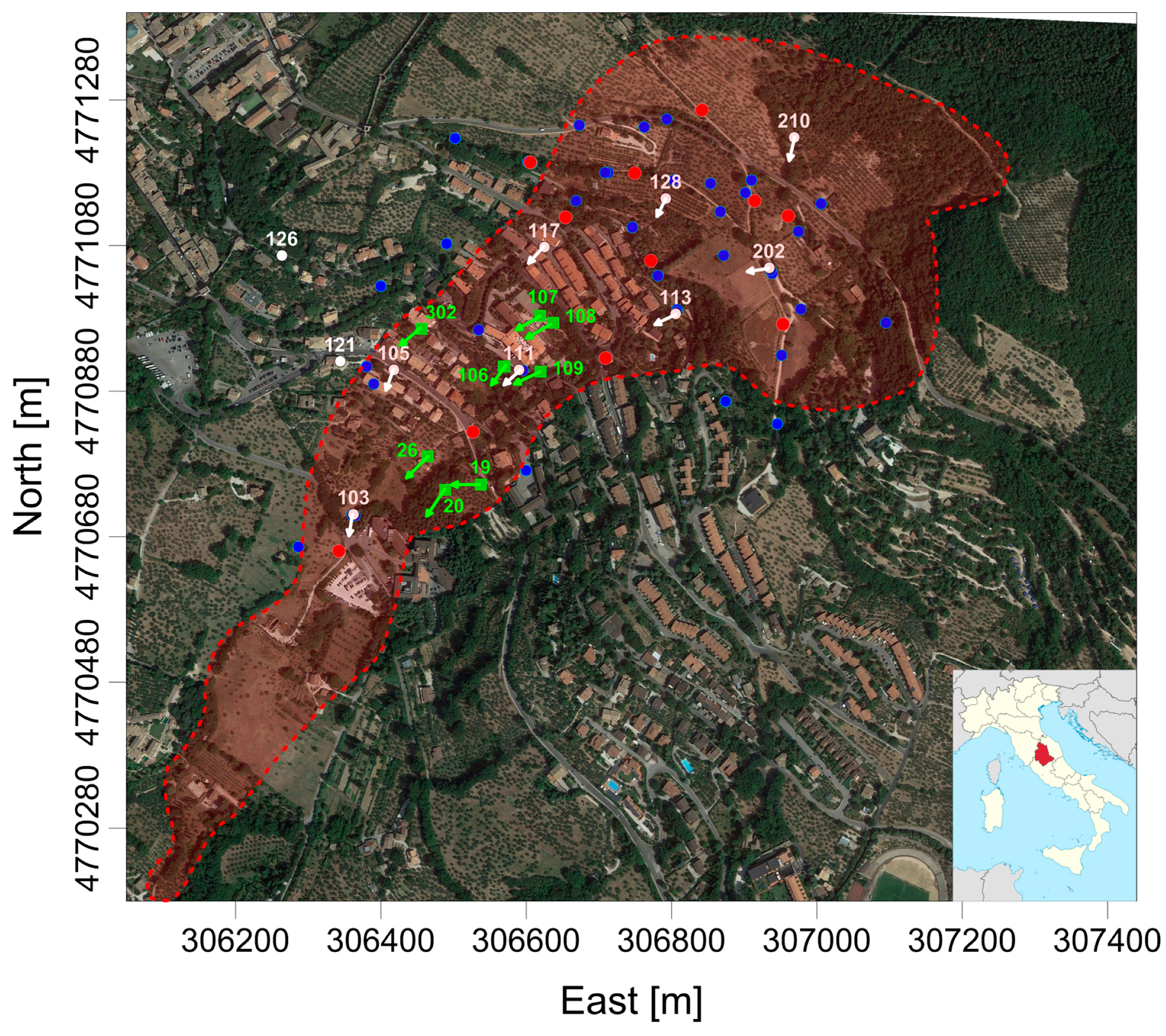
The present work (the Ivancich landslide, which affects a residential area outside the historical center of the Assisi town, Central Italy), has been selected as a representative case study to highlight the capability of advanced three-dimensional FE modeling as a complementary tool in performing an effective risk analyses of the slow landslide processes and accurate urban development planning (
Figure 1).
The Ivancich landslide is an ancient landslide phenomenon and consists of a slow deep-seated mass movement, which can be classified as a typical earth-slide [
19]. Although the rate of movement is very slow, the landslide has caused major damage to buildings, roads and infrastructures due to the effect of accumulation of ground differential displacements over time [
20,
21]. The first evidence of landslide activity were recorded in 1399 on the ancient Franciscan convent, which represented at that time the only anthropic structure of the area. In accordance with the demographic development that followed the end of World War II, the town of Assisi and its surrounding was intensely urbanized. Consequently around 1970, further evidence of landslide mobility started to appear in the form of growing damage to buildings, retaining walls, pipelines and road paving. The infrastructure damage led local authorities in carrying out several geological and geotechnical investigations aimed at studying the landslide process and designing the mitigation strategies [
20,
22]. Indeed, the area has been deeply investigated over the last 20 years and extensively monitored through in situ inclinometers, piezometers and GPS measurements [
23,
24,
25]. At the same time, remote sensing techniques have been exploited in order to achieve dense spatial information of the unstable mass [
18,
26]. Such a large availability of measurements and in situ data makes the Ivancich landslide a real-scale laboratory in order to test and validate new approaches and techniques based on the integration of multi-source data. In this scenario, the FE modeling approach, based on the integration of available geological, geotechnical and satellite dataset, is aimed at investigating the 3D kinematical evolution of the landslide in the different sectors of the instability process. In particular, we exploit 39 SAR images collected by the Cosmo-SkyMed (CSK) constellation in the 2009–2012 time period, 7 litho-stratigraphic cross-sections and 62 stratigraphic boreholes.
Finally, the achieved outcomes allow us to investigate the spatial and temporal evolution of the slope affected by slow-moving phenomenon and via comparison with the geomorphological data, to derive insights into the kinematical activity map of the whole area affected by the Ivancich landslide.
3. Three-Dimensional Finite Element Modeling
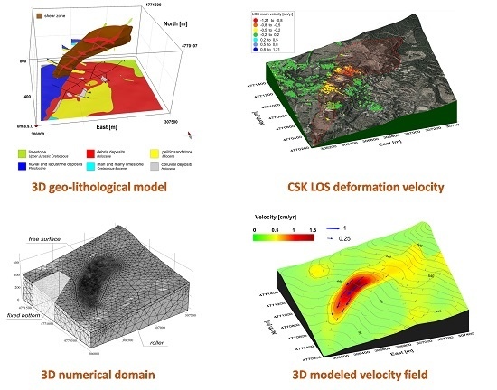
In this work, we exploit a numerical approach based on an optimized three-dimensional FE model that is constrained by DInSAR and field measurements. In particular, we combine the benefits of a deterministic numerical approach with statistical methods aimed at improving and optimizing the obtained numerical solution in order to analyze and interpret the ground deformations measured in the whole landslide area.
Based on the linearity of kinematics affecting the unstable mass, as observed according to the landslide monitoring dataset, we carry out the three-dimensional FE modeling of the active ground deformation field by assuming, as a first approximation, the soil material behavior as Newtonian fluid characterized by viscosity constant over time. We remark that this model can be applied mainly to landslide cases where the shear zone geometry is well formed and well known by means of accurate and detailed in-situ investigations. In this scenario, the distribution of the soil viscosity parameter within the whole numerical domain can be evaluated through an advanced procedure that implements a nonlinear optimization of the model parameters aimed at simulating the CSK DInSAR measurements. Accordingly, we can assume a steady-state viscous flow (Newtonian fluid) solved through the incompressible Navier–Stokes differential equations:
where
u [m/s] is the deformation velocity vector;
F [Pa/m] is the body force term;
ρ [kg/m
3] is the density; p [Pa] is the pressure; and
μ is the dynamic viscosity [Pa·s] (hereafter referred to as viscosity) [
34].
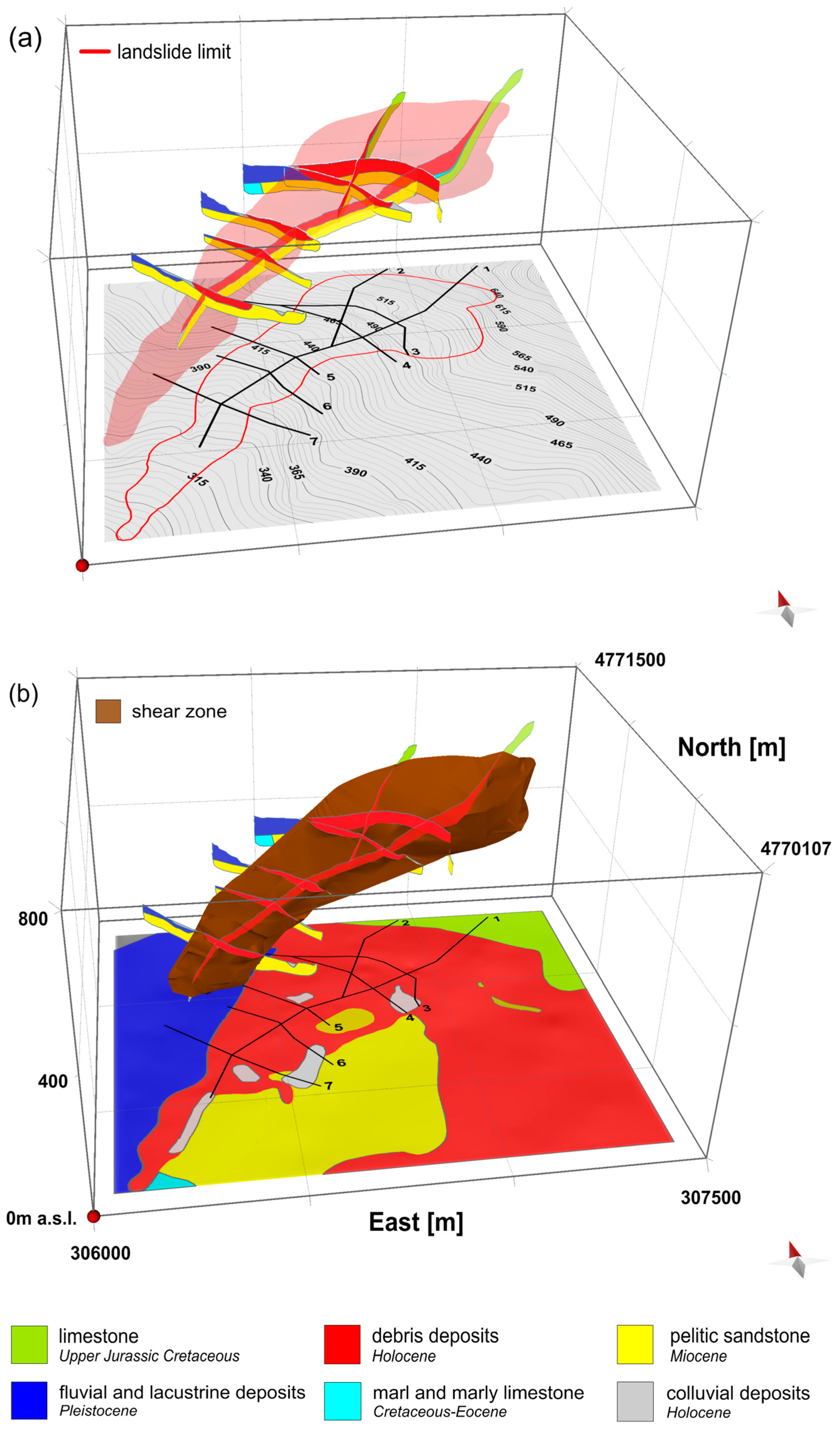
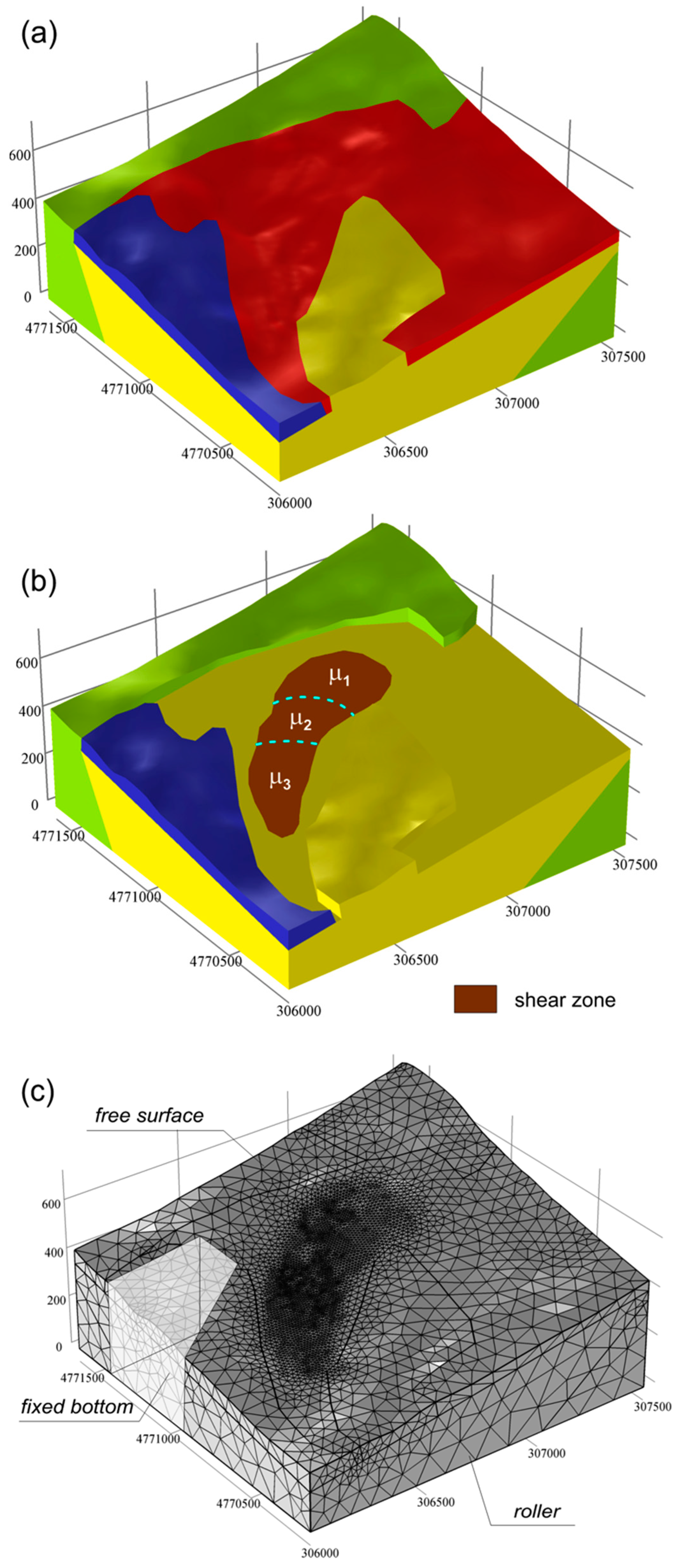
The first step of the analysis deals with the setup of the a priori geo-lithological model. The interpretation of the available geological data provides a more accurate insight on the landslide geological conditions, as well as a more effective view capability of complex geological processes. In particular, in a geo-referenced system, the DEM (Digital Elevation Model), the geological map, the lithological cross-sections and the inclinometric borehole data are taken into account (
Figure 4a,b) to define a realistic 3D geo-lithological model (1.5 × 1.5 × 0.1 km
3) of the Ivancich area.
Consequently, we have implemented the 3D geo-lithological model of the whole landslide divided into five geo-mechanical units within a numerical environment (see
Table 1 for the corresponding physical properties): the limestone bedrock, in the upper part of the slope; the pelitic sandstone bedrock in the central and lower portions of the slope; the landslide deposit formed of unsorted debris; the colluvial deposit in the landslide toe area; the shear zone characterized by thickness of less than 2 m at depths ranging between 15 and 60 m from the ground surface.
The performed 3D geo-lithological model allows us to finely define the geometric features of the shear zone beneath the landslide deposit. Subsequently, we divided the shear zone into three sectors characterized by a homogenous viscosity value (
Figure 4b), in accordance with both the geomorphological features along the slope and the kinematical behavior observed for the different portions of the landslide. The evidence of the existence of different landslide kinematical sectors is also supported by the analysis of the DInSAR measurements, which proves that the identified sectors are characterized by different kinematical rates.
We remark that such an accurate definition of the shear zone domain is not possible in the 2D scenario [
8], that represents, for the lack of geometrical constraints along the considered section, a rougher model. However, it is worth noting that the proposed subdivision has no significant impact on the applicability of the method and a finer discretization, although involving an increase of the computational load, can be easily applied in more complex scenarios.
The 3D numerical domain is discretized by creating a mesh that consists of about 620,000 tetrahedral elements. The element sizes range from 2 to 200 m; moreover, a mesh refinement was applied within the shear-zone domain where higher deformation rates were expected. The generated mesh is then validated through several resolution tests [
35,
36], which indicate a negligible mesh-dependency of the solution, since the use of a finer mesh would have affected the results by less than 2%.
Regarding the boundary conditions, the upper part of the geometry model which represents the ground surface of the slope, is considered as unconstrained (free surface); the bottom boundary is fixed. The four lateral side boundaries are instead characterized by null horizontal displacement. Finally, the inner domain is characterized by continuity between the different geological units.
According to Griffiths and Lane [
37], we perform our modeling in two stages: gravity loading, aimed at defining a stress field representative of the current stress state of the slope; landslide process, i.e., the kinematics simulation. During the gravity loading, the stress state of the slope is defined by considering the slope as subjected to the soil gravitational loads and assuming elastic soil behavior. At this level, only the generated stress field is considered while the nodal displacements are kept equal to zero. In the landslide process, the previously calculated stresses are applied to the whole domain and the Newtonian approach is considered to simulate the kinematical trend of the landslide during the 2009–2012 time interval. The analysis implicitly assumes that the landslide body, delimited by the underlying shear zone, is unstable or marginally stable: this is specifically verified by means of a limit equilibrium calculation that provided a stability factor of the landslide body close to unity. It is worthwhile stressing that for the considered Newtonian viscous flow, soil is assumed to behave as a single-phase material. As described before, this assumption is supported by the available open-pipe piezometric measurements (
Supplementary Materials Figure S2), locally indicating moderate variations of the water level within the landslide debris and by electric piezometer measurements showing very low variations of the pore water pressure at the depth of the shear band. Accordingly, we can assume that the pore water pressure regime plays a minor role in the landslide evolution process and separation between pore fluid and soil skeleton behavior is not needed for the present study. Note that, in order to simulate the landslide debris movement approximately as a rigid body, in the considered physical context the viscosity values of the layers overlaying the shear domain (surrounding rocks) are chosen with different order of magnitude (
Table 1).
In order to integrate all the available data described in
Section 2 and solve the field Equation (1), the COMSOL Multiphysics finite-element modeling code is used.
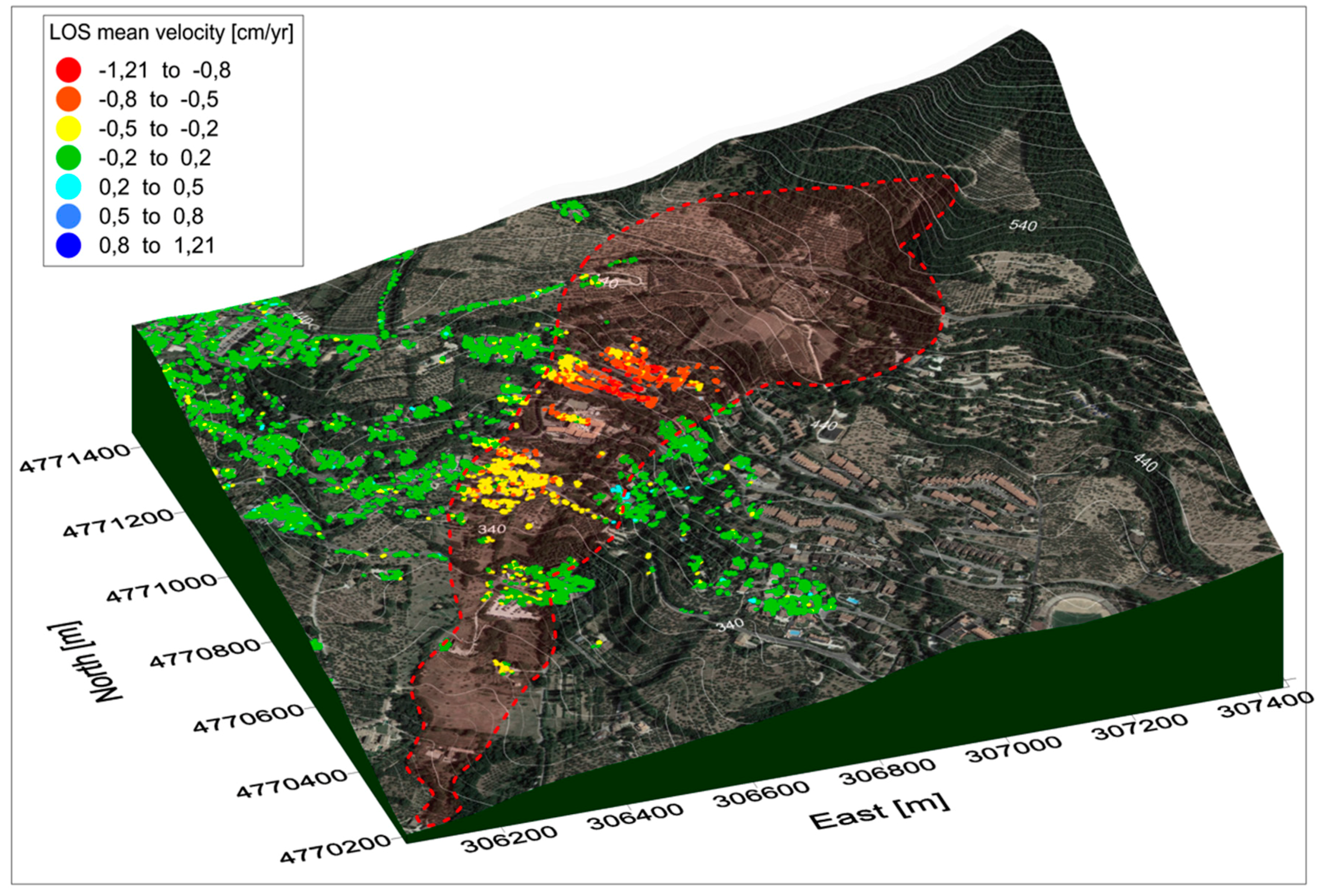
The modelled displacement rates are evaluated at the topographic surface, projected along the satellite line of sight (LOS) and compared with the DInSAR measurements. In particular, the optimization procedure is performed by exploiting the CSK SBAS-DInSAR results (
Figure 3). To detect the model providing the best agreement between DInSAR measurements and FE model, we use the Monte Carlo statistical method, which is based on the exploration of the parameter values in a defined space of variables (coordinate search method) [
38,
39]. This procedure allows us to find, for the three different shear band sectors, the viscosity parameters that correspond to the model that best-fits the DInSAR measurements. To evaluate the similarity between the data vs. model, we use the Root Mean Square Error (RMSE) cost function; it is represented by a weighted average of the residuals, expressed as:
where
di,obs and
di,mod are the observed and modeled displacement of the
i−th point,
σi is the standard deviation for the
N points.
4. Results
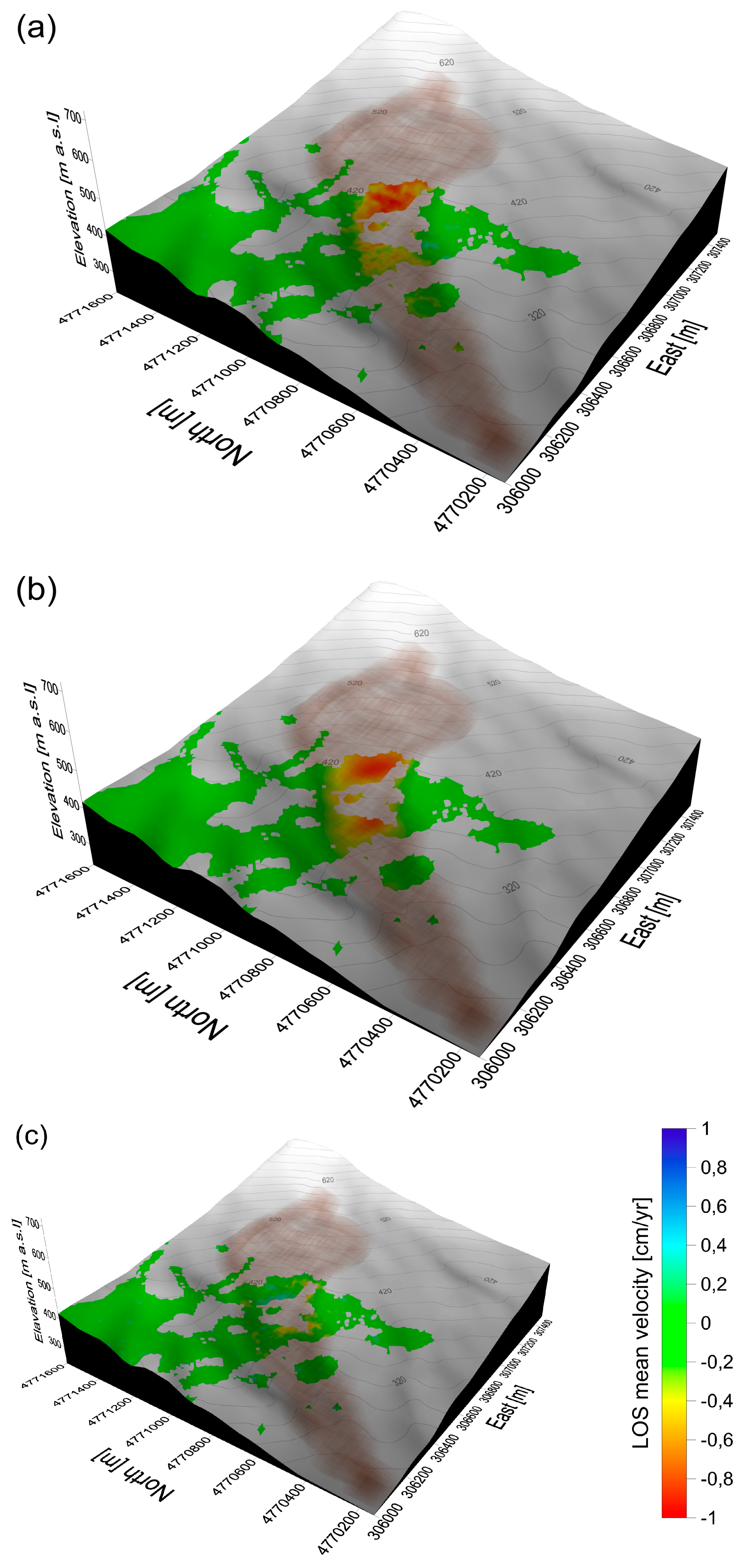
A quantitative comparison between the CSK SBAS-DInSAR measurements (
Figure 5a) and the achieved model results projected along LOS (
Figure 5b), computed in correspondence of the SAR coherent pixels is performed; the
Figure 5c represents the difference (residuals) between data and model results. The residuals map (
Figure 5c) shows the good fit between data and model results, revealed also by the RMSE value that is equal to 0.15 cm/yr, smaller than the accuracy of the SBAS-DInSAR measurements [
28]. In addition, the performed analysis also provides a good temporal fit between the DInSAR deformation time series and the modeled one for the considered time interval (
Supplementary Materials Figure S1).
Starting from the analysis that best-fits the displacement monitoring data, we evaluate the related viscosity parameters of the three sector of shear zone (
µ1,
µ2,
µ3). The corresponding estimated values are reported in
Table 2, along with the initial ranges adopted for the analysis.
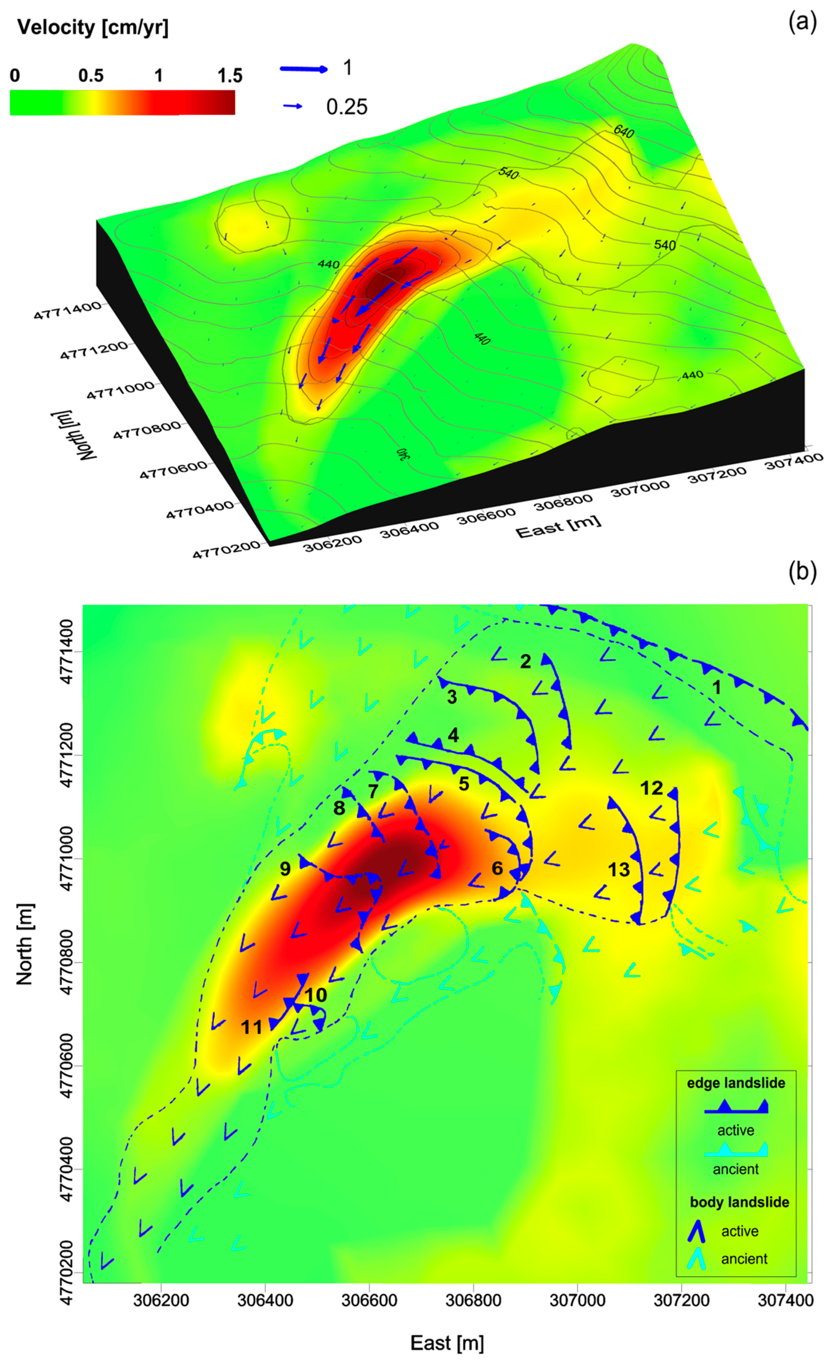
The optimized FE model allows for the analysis of the overall ground velocities field. In
Figure 6a we show the amplitude and direction of the achieved velocity field; in this map the amplitude of the velocity field reaches a maximum value of 1.5 cm/yr at altitudes between 320 and 400 m a.s.l., in the middle-upper part of the unstable area. In addition, the model results well represent the slight curvature in the horizontal plane of the landslide process along the South-East direction, as also highlighted by the modeled vectors (
Figure 6a). A comparative analysis between the morphological units of the Ivancich slope (ancient and active edges landslide) as proposed by Pontoni [
23,
24] and the model results are also reported (
Figure 6b); more than the 70% of the mapped geomorphological structures (units 6–11) are enclosed in the region where the 2009–2012 deformation process is active. The units 12 and 13 are marginally involved while the units 1–4 seem to be not active in the considered time interval (with mean velocity lower than 0.3 cm/yr). Our analysis also highlights the existence of a spatially correlated deformation pattern (0.5 cm/yr) superimposed on the cataloged ancient structures located in the North Western region of the landslide slope.
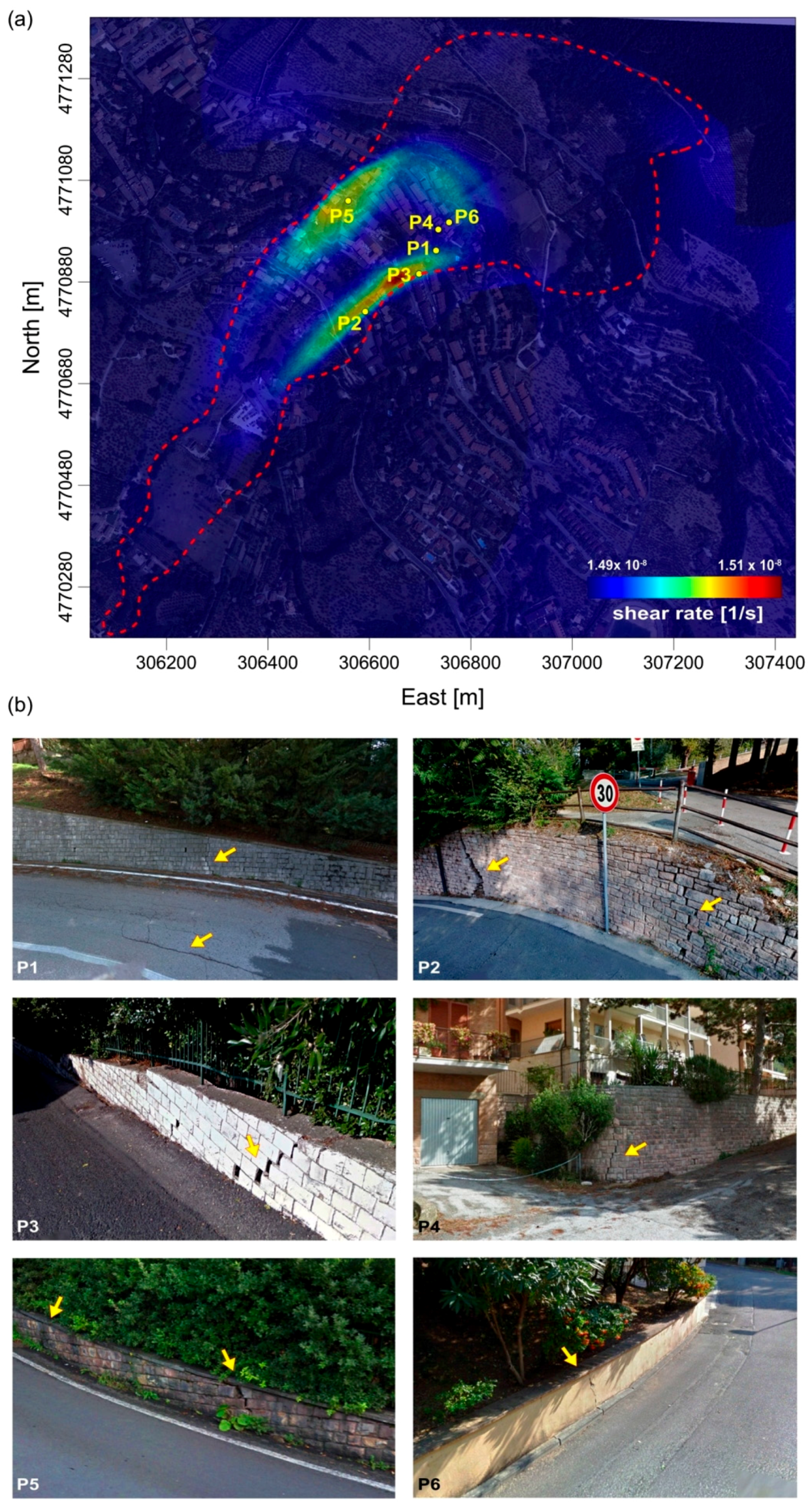
Finally, we show a map with the computed shear rate values (
Figure 7a) that represents the ratio of the shear stress to the dynamic viscosity. It is interesting to note that the landslide portions where the structures are damaged, as many photographs recorded in the Ivancich surroundings clearly show (
Figure 7b), are in accordance with the distribution of the anomaly of the shear rate. In fact, serious damage corresponding to the P2, P3 and P5 sites are localized along the landslide boundaries and in correspondence of highest values of shear rate.
5. Discussion
In this work, we perform a three-dimensional optimized model based on a fluid-dynamic physical scenario realizing an effective integration of satellite and terrestrial observations in the FE environment. In detail, based on the linearity of kinematics affecting the unstable mass as ensured by the DInSAR deformation time-series, we can assume the soil material behavior as Newtonian fluid, characterized by the viscosity parameter constant over time. Despite that, the Newtonian fluid assumption is not a rigorous constitutive model for the soil physical proprieties, it is useful to simulate the landslide kinematical behavior; we remark that this model can be applied only to a landslide-type where the shear zone geometry is well formed and well known by means of accurate and detailed in-situ investigations (
Figure 2).
In this perspective, a three-dimensional kinematical model is performed, providing a full map of the current landslide velocities, both in terms of modules and corresponding directions. A spatial kinematic variability is also highlighted from the retrieved velocity map, since lower velocities are calculated along the lateral boundaries of the landslide with respect to the inner portions. The consistency of the model results with respect to the DInSAR velocity field (
Figure 5) also represents a further back-validation of the 3D shear zone geometry. In addition, we compare the modeled velocity pattern with the main geomorphological features of the Ivancich slope (ancient and active edges landslide) highlighting a good match. In fact, the analysis reveals that more than the 70% of the mapped geomorphological structures are still active. The existence of a stable geological element made of in-place pelitic sandstone, along the left-hand side of the landslide at middle elevations, probably influences the direction of the phenomenon toward South-East, as supported by the geomorphological features of the study area (
Figure 6). Moreover, we correlate the additional damage and the modeled shear rate. This study reveals that ruptures are most severe along the landslide boundaries between active and inactive sectors; this result is expected when the spatial gradient of the modeled velocities field in maximum (
Figure 7). We argue that the information on the average landslide velocities and shear rate can provide an important contribution into predicting possible deformation scenarios for structures and infrastructures lying within the landslide area and for the land management of the whole area. Our results furnish a promising support for risk analysis of very slow landslides within a reasonable time span and for which the analysis can be considered as an expected representation of the coming years.
In order to show the advance of our 3D modeling respect to the 2D FE ones [
8,
18], we perform a comparative analysis between the retrieved velocity fields reported in
Supplementary material (Figure S3). The achieved results point out a significant improvement of the residual values. It is worthwhile pointing out that the 3D optimized viscosity values are lower than those achieved via 2D modeling. These discrepancies could be related to: (i) the effect of the detailed shear zone geometry; (ii) a different confining effect and stress field of the three-dimensional model respect to the two-dimensional one. However, these results emphasize how the modeling approach is strongly influenced by the type of the performed dimensional analysis.
6. Conclusions
The achieved results clearly demonstrate how the integration of remote sensing, in-situ monitoring and FE modeling is strategic in performing detailed analyses of complex deformation scenarios. By benefiting from three-dimensional advanced modeling tools we can effectively investigate the overall mechanism of the evolution of the ground displacements related to slow landslide phenomena, as well as outline possible risk scenarios. As a matter of fact, if in-situ measurements or DInSAR-based analyses are capable of exploring the displacement trends of specific sectors of a landslide process, the three-dimensional model can provide a thorough physically-based conceptualization of the landslide kinematics, provided that the same model is calibrated and optimized against the aforementioned measurements.
The calibrated three-dimensional FE model provides more opportunities as a zonation tool capable of identifying and updating the status of the morphological structures originally mapped from in-situ investigations. The amplitude of the velocity field reaches a maximum value of 1.5 cm/yr at altitudes between 320 and 400 m a.s.l., in the middle-upper part of the unstable area; more than the 70% of the mapped geomorphological structures are enclosed in the region where the 2009–2012 deformation process is active. The model fully delineates the landslide portions that are subjected to different landslide velocities and this can be useful for land management purposes; therefore, the comparison between the 3D vs. 2D model results highlights that the sliding surface, calculated via the 3D geo-lithological model, is more realistic in respect to those realized in the 2D model.
Finally, we remark that the damage analysis detected in the Ivancich surroundings compared with the three-dimensional FE model results, reveals that ruptures are most severe along the boundary between active and inactive landslide sectors where the shear rate values are high. Hence, the proposed three-dimensional FE modeling tool represents a valuable support for landslide risk analyses and urban development planning within a specific territory area affected by complex slow-moving landslide processes.


 ,
, 


