
How Universal Is the Relationship between Remotely Sensed Vegetation Indices and Crop Leaf Area Index? A Global Assessment

 , , , ,
  ,
,
Abstract
:
1. Introduction
2. Data and Methodology
2.1. LAI data Collection and Quality Control
2.2. Remotely Sensed Data
2.3. Establishment of the Global LAI-VI Relationships
2.3.1. Exploratory Analysis: Symbolic Regression
2.3.2. Refined Models of LAI-EVI and LAI-EVI2 relationships
2.4. Evaluation of the Global LAI-VI Relationships
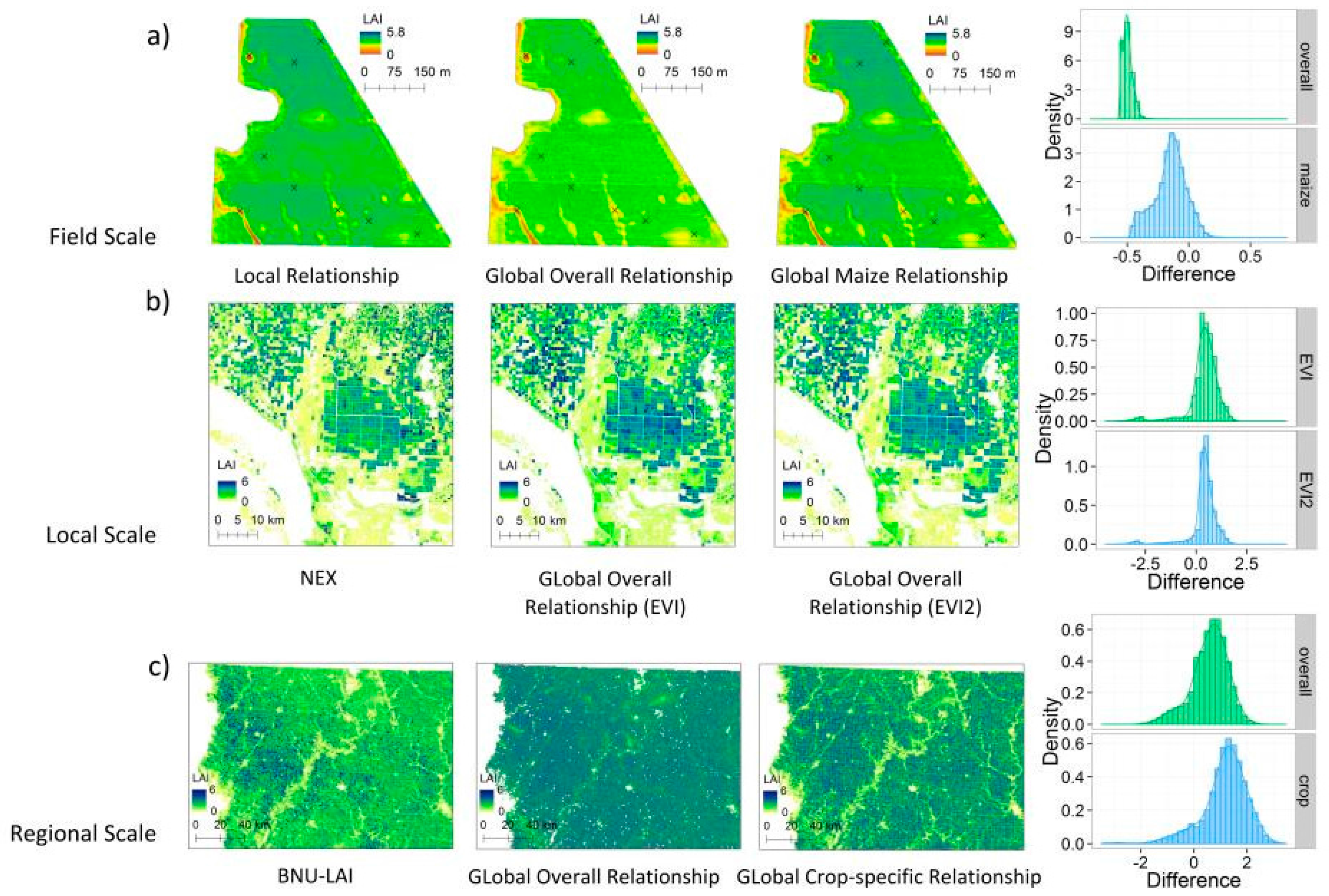
2.5. Preliminary Validation and Example Applications at Three Spatial Scales
2.5.1. Field Scale Application
2.5.2. Local Scale Application
2.5.3. Regional Scale Application
3. Results
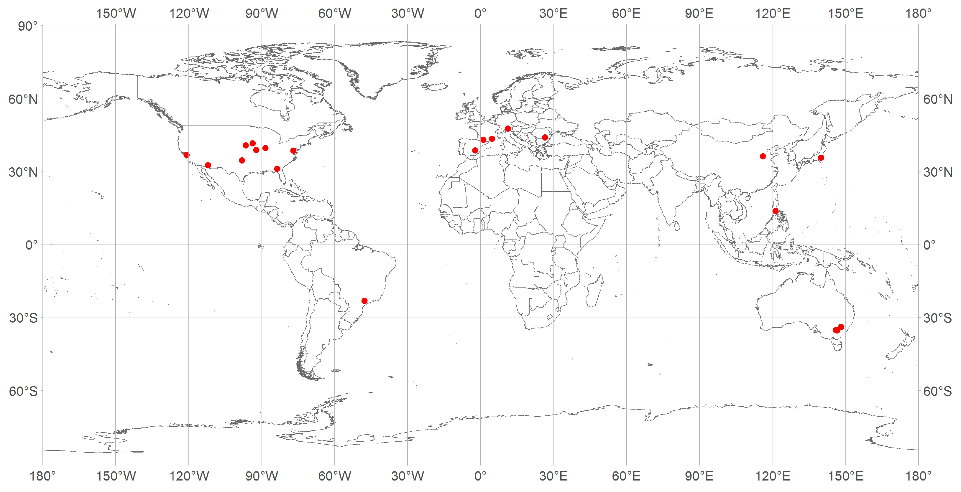
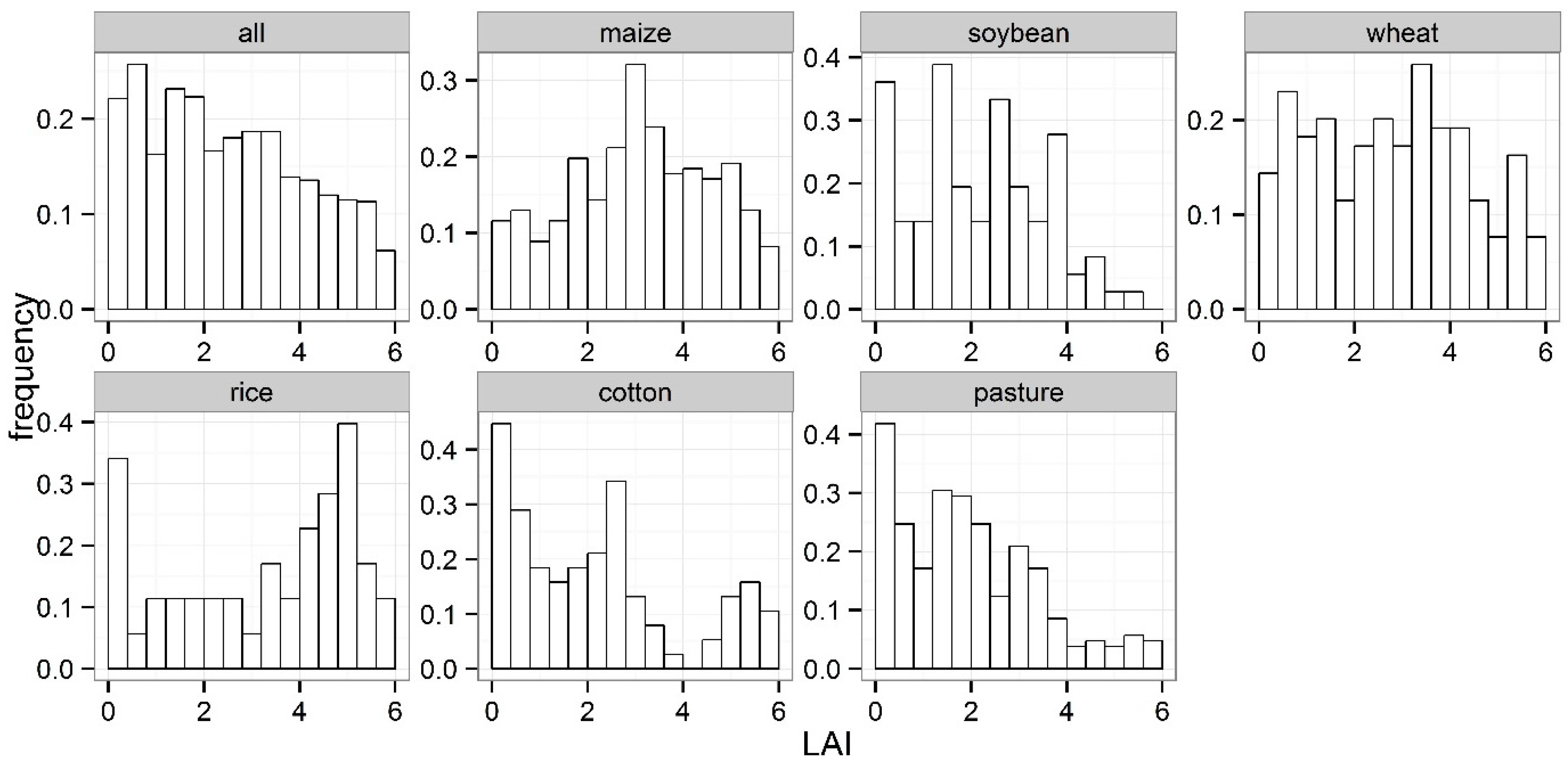
3.1. Description of the In-Situ LAI Data Set
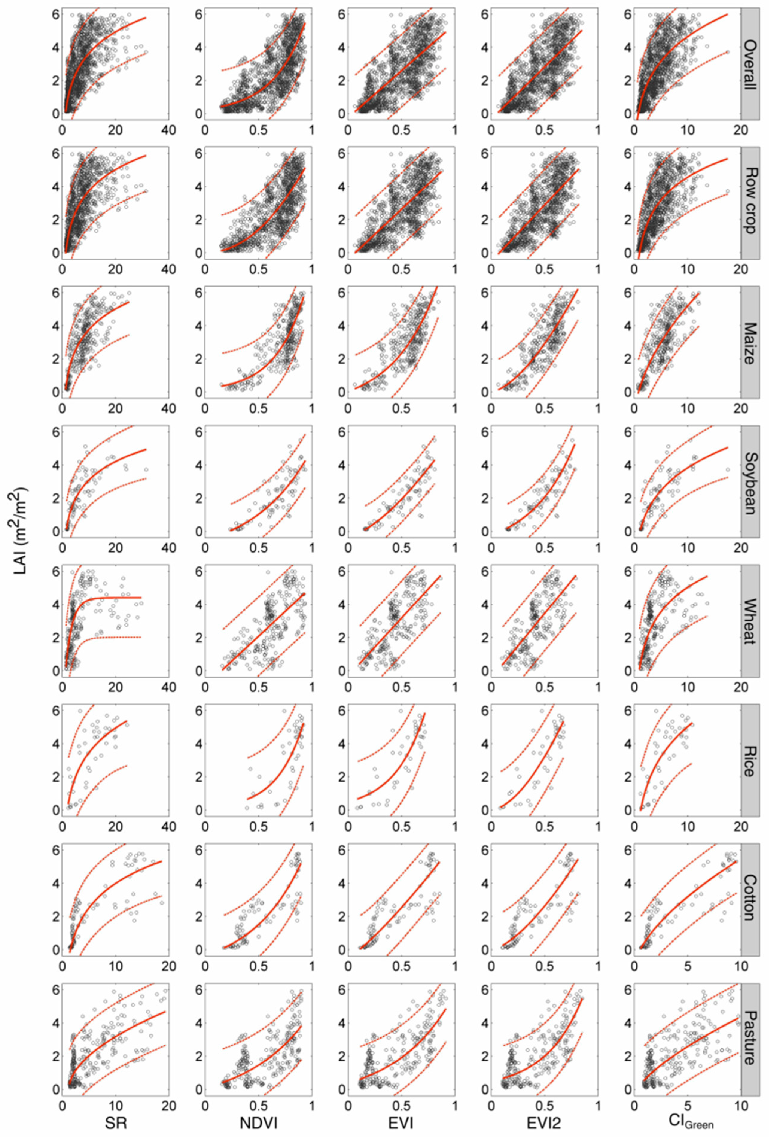
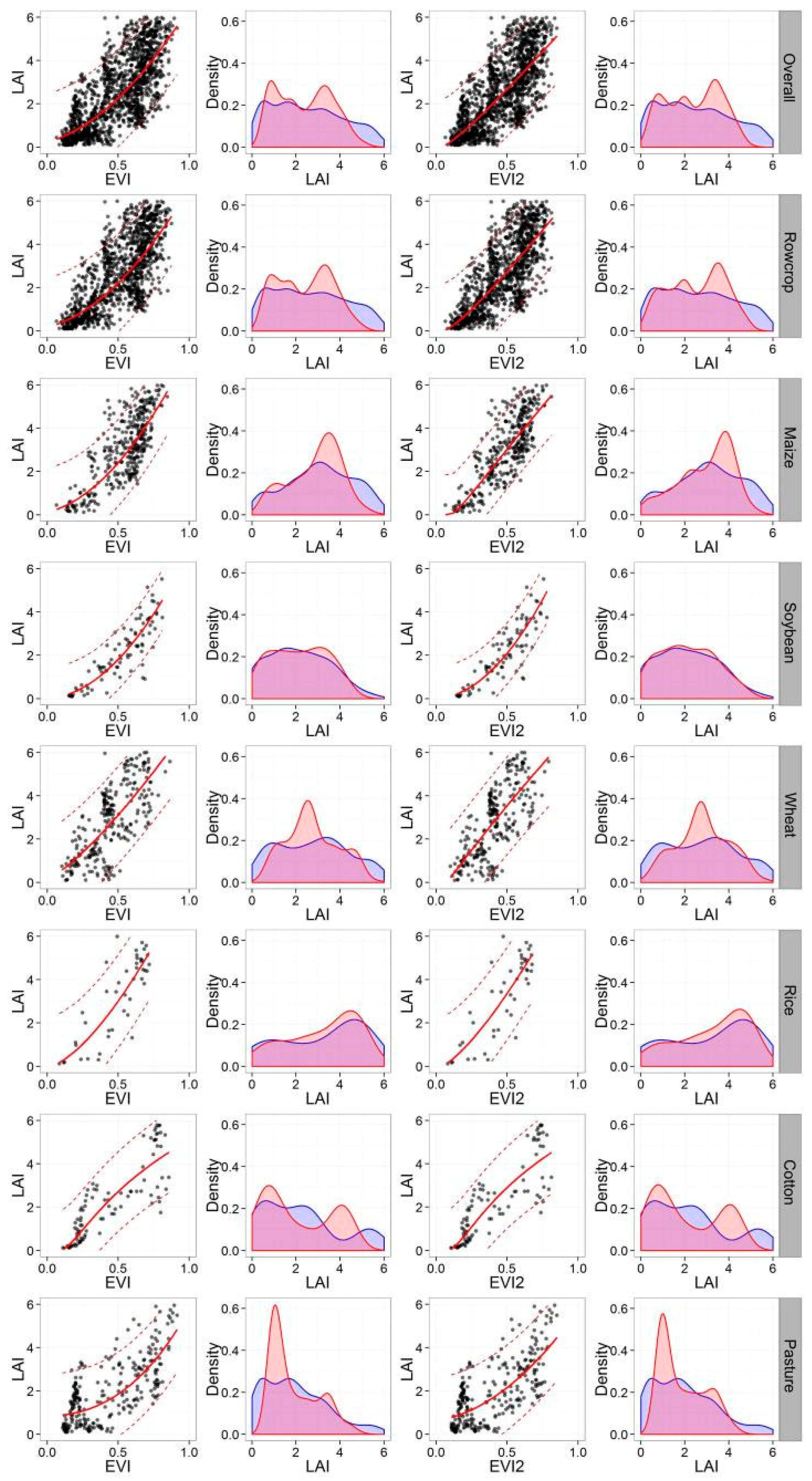
3.2. Exploratory Analysis of the LAI-VI Relationships
3.2.1. Form and Shape of the Best-Fit-Functions
3.2.2. GOF Metrics of the Best-Fit-Functions
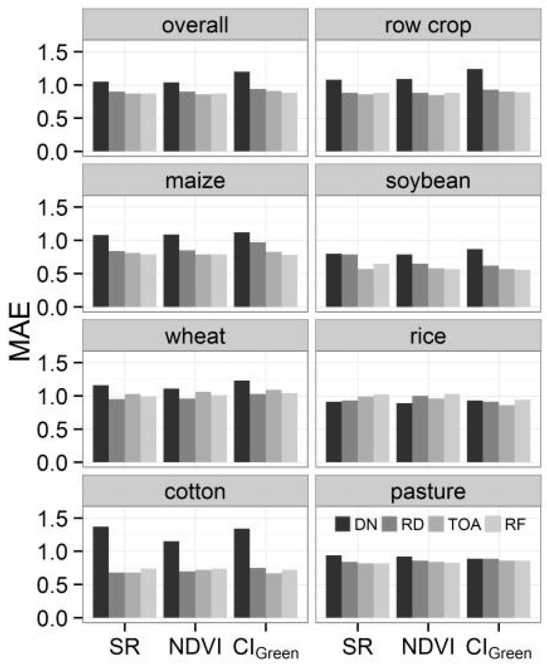
3.2.3. The Effect of Levels of Radiometric/Atmospheric Corrections
3.2.4. The Best-Fit Functions Based on Full-Range Dataset
3.3. LAI-EVI and LAI-EVI2 Relationships Based on Theil-Sen Regression
3.4. Evaluation of the LAI-EVI/EVI2 Relationships
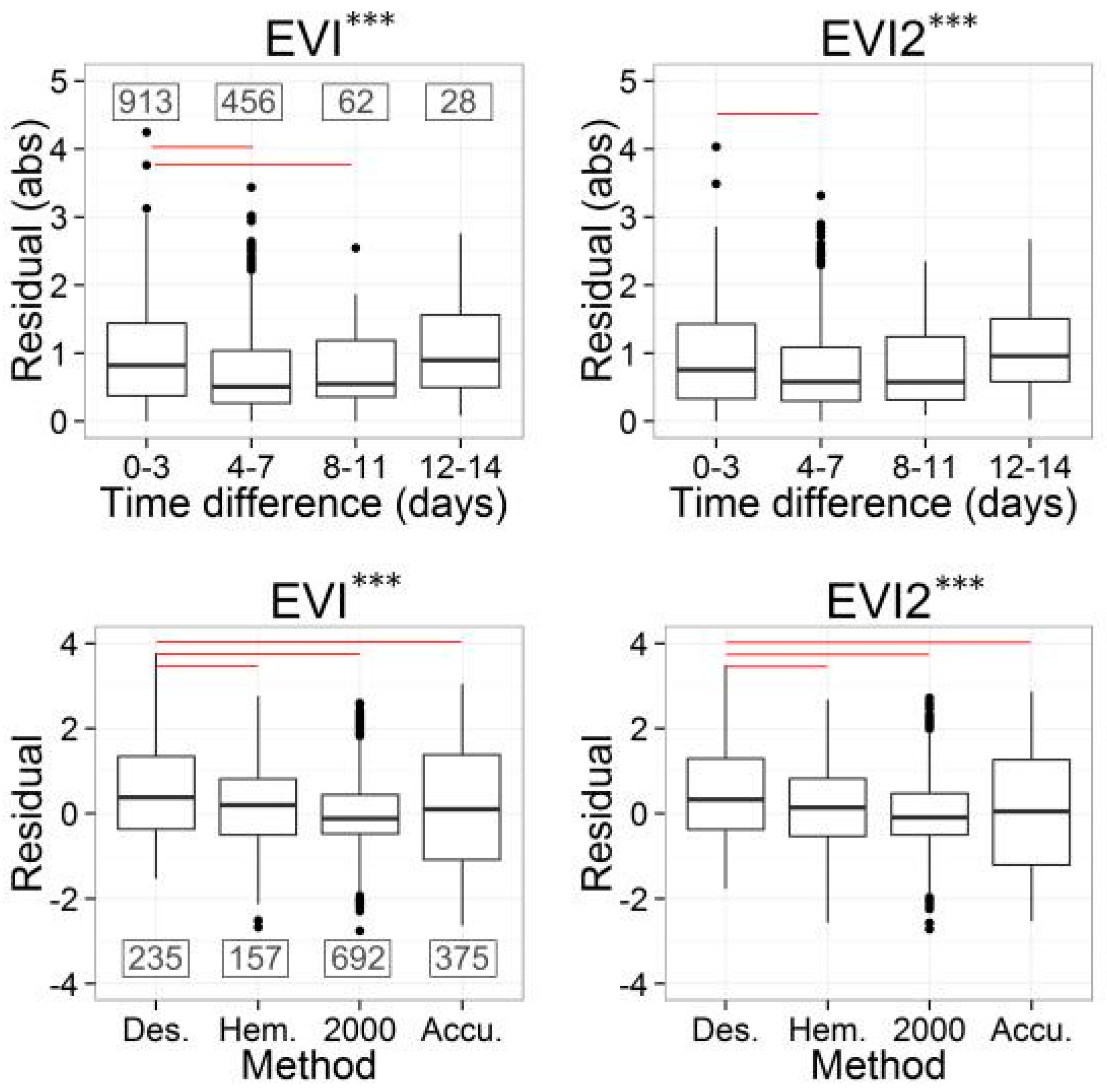
3.4.1. Analysis of the Errors from Temporal Mismatch and Measurement Methods
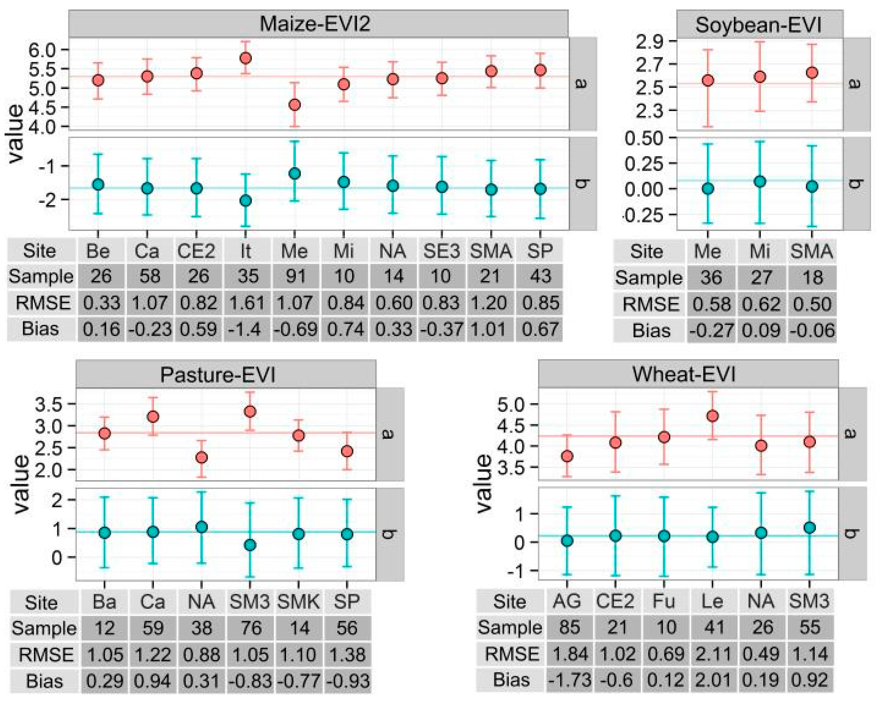
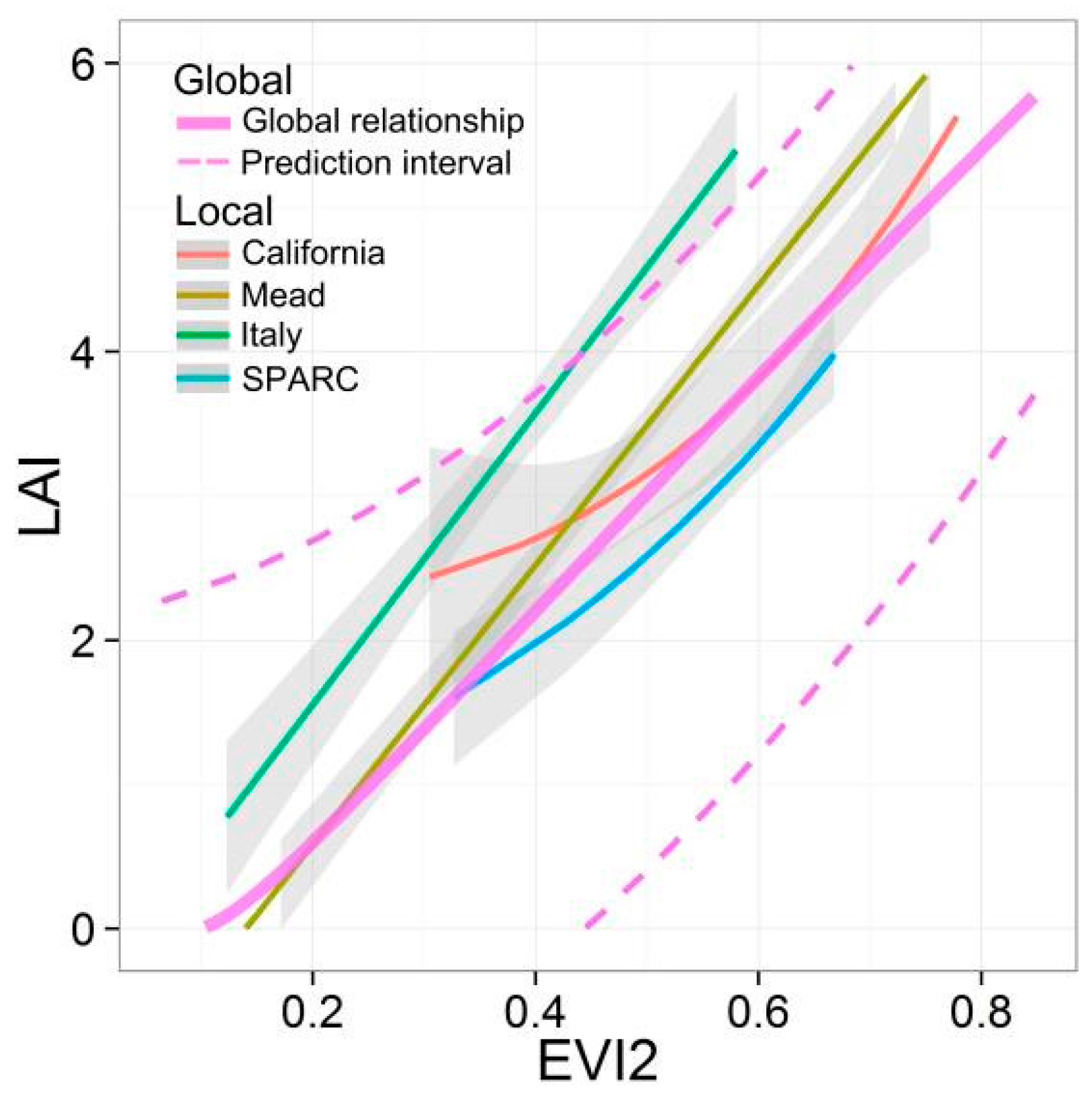
3.4.2. Site-Based Evaluation on Global Universality
3.5. Preliminary Validation and Example Applications
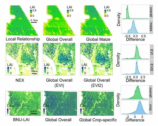
3.5.1. Field Scale
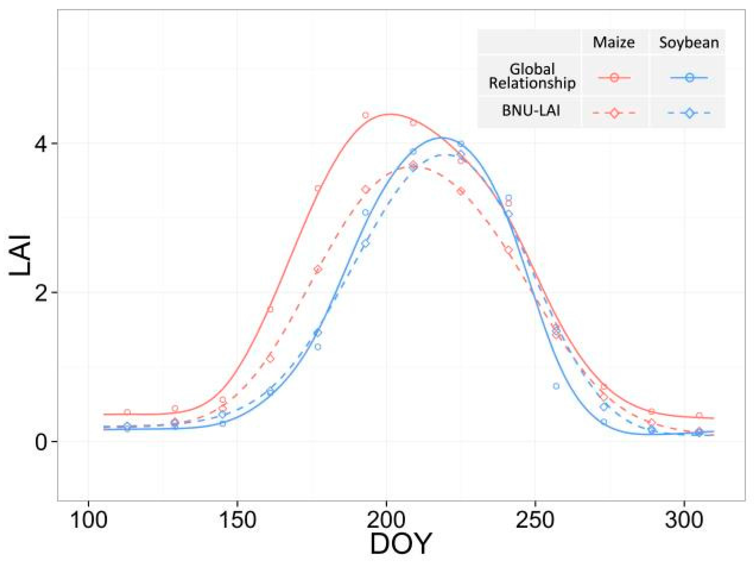
3.5.2. Local Scale
3.5.3. Regional Scale
4. Discussion
4.1. Universality vs. Diversity
4.2. Considerations in the Validation of the Global LAI-VI Relationships
4.3. Potential Issues Related to Data Quality and Consistency
4.4. Concerns in the Model Prediction Power
5. Conclusions
Supplementary Materials
Acknowledgments
Author Contributions
Conflicts of Interest
References
- Watson, D.J. Comparative physiological studies on the growth of field crops: I. variation in net assimilation rate and leaf area between species and varieties, and within and between years. Ann. Bot. 1947, 11, 41–76. [Google Scholar] [CrossRef]
- Fernandes, R.; Plummer, S.; Nightingale, J.; Baret, F.; Camacho, F.; Fang, H.; Garrigues, S.; Gobron, N.; Lang, M.; Lacaze, R.; et al. Global Leaf Area Index Product Validation Good Practices. Version 2.0. In Best Practice for Satellite-Derived Land Product Validation; Schaepman-Strub, G., Román, M., Nickeson, J., Eds.; Land Product Validation Subgroup (WGCV/CEOS), 2014; p. 76. Available online: http://lpvs.gsfc.nasa.gov/documents.html (accessed on 11 April 2013). [Google Scholar] [CrossRef]
- Launay, M.; Guerif, M. Assimilating remote sensing data into a crop model to improve predictive performance for spatial applications. Agric. Ecosyst. Environ. 2005, 111, 321–339. [Google Scholar] [CrossRef]
- Food and Agriculture Organization of the United Nations (FAO). Terrestrial Essential Climate Variables for Climate Change Assessment, Mitigation and Adaptation; FAO: Rome, Italy, 2008. [Google Scholar]
- Anav, A.; Murray-Tortarolo, G.; Friedlingstein, P.; Sitch, S.; Piao, S.; Zhu, Z. Evaluation of Land Surface Models in Reproducing Satellite Derived Leaf Area Index over the High-Latitude Northern Hemisphere. Part II: Earth System Models. Remote Sens. 2013, 5, 3637–3661. [Google Scholar] [CrossRef]
- Koetz, B.; Baret, F.; Poilvé, H.; Hill, J. Use of coupled canopy structure dynamic and radiative transfer models to estimate biophysical canopy characteristics. Remote Sens. Environ. 2005, 95, 115–124. [Google Scholar] [CrossRef]
- Gitelson, A.A.; Peng, Y.; Arkebauer, T.J.; Schepers, J. Relationships between gross primary production, green LAI, and canopy chlorophyll content in maize: Implications for remote sensing of primary production. Remote Sens. Environ. 2014, 144, 65–72. [Google Scholar] [CrossRef]
- Bondeau, A.; Kicklighter, D.; Kaduk, J. Comparing global models of terrestrial net primary productivity (NPP): Importance of vegetation structure on seasonal NPP estimates. Glob. Chang. Biol. 1999, 5, 35–45. [Google Scholar] [CrossRef]
- Asner, G.P.; Scurlock, J.M.O.; Hicke, J.A. Global synthesis of leaf area index observations: Implications for ecological and remote sensing studies. Glob. Ecol. Biogeogr. 2003, 12, 191–205. [Google Scholar] [CrossRef]
- Ines, A.V.M.; Das, N.N.; Hansen, J.W.; Njoku, E.G. Assimilation of remotely sensed soil moisture and vegetation with a crop simulation model for maize yield prediction. Remote Sens. Environ. 2013, 138, 149–164. [Google Scholar] [CrossRef]
- Cao, X.; Zhou, Z.; Chen, X.; Shao, W.; Wang, Z. Improving leaf area index simulation of IBIS model and its effect on water carbon and energy—A case study in Changbai Mountain broadleaved forest of China. Ecol. Model. 2015, 303, 97–104. [Google Scholar] [CrossRef]
- Curran, P.; Steven, M. Multispectral remote sensing for the estimation of green leaf area index. Philos. Trans. R. Soc. Lond. Ser. A Math. Phys. Sci. 1983, 309, 257–270. [Google Scholar] [CrossRef]
- Myneni, R.B.; Ramakrishna, R. Estimation of global leaf area index and absorbed PAR using radiative transfer models. IEEE Trans. Geosci. Remote Sens. 1997, 35, 1380–1393. [Google Scholar] [CrossRef]
- Gower, S.; Kucharik, C.; Norman, J. Direct and Indirect Estimation of Leaf Area Index, f APAR, and Net Primary Production of Terrestrial Ecosystems. Remote Sens. Environ. 1999, 70, 29–51. [Google Scholar] [CrossRef]
- Gobron, N.; Verstraete, M.M. Assessment of the status of the development of the standards for the Terrestrial Essential Climate Variables LAI (No. T11). Rome, 2009. Available online: http://www.fao.org/gtos/doc/ECVs/T11/T11.pdf (accessed on 12 April 2013).
- Guindin-Garcia, N.; Gitelson, A.A.; Arkebauer, T.J.; Shanahan, J.; Weiss, A. An evaluation of MODIS 8- and 16-day composite products for monitoring maize green leaf area index. Agric. For. Meteorol. 2012, 161, 15–25. [Google Scholar] [CrossRef]
- Bréda, N.J.J. Ground-based measurements of leaf area index: A review of methods, instruments and current controversies. J. Exp. Bot. 2003, 54, 2403–2417. [Google Scholar] [CrossRef] [PubMed]
- Jonckheere, I.; Fleck, S.; Nackaerts, K.; Muys, B.; Coppin, P.; Weiss, M.; Baret, F. Review of methods for in situ leaf area index determination. Agric. For. Meteorol. 2004, 121, 19–35. [Google Scholar] [CrossRef]
- Baret, F.; Guyot, G. Potentials and limits of vegetation indices for LAI and APAR assessment. Remote Sens. Environ. 1991, 35, 161–173. [Google Scholar] [CrossRef]
- Carlson, T.; Ripley, D. On the relation between NDVI, fractional vegetation cover, and leaf area index. Remote Sens. Environ. 1997, 62, 241–252. [Google Scholar] [CrossRef]
- Jacquemoud, S.; Bacour, C.; Polive, H.; Frangy, J.P. Comparison of four radiative transfer models to simulate plant canopies reflectance: Direct and inverse mode. Remote Sens. Environ. 2000, 74, 471–481. [Google Scholar] [CrossRef]
- Buermann, W.; Dong, J.; Zeng, X. Evaluation of the utility of satellite-based vegetation leaf area index data for climate simulations. J. Clim. 2001, 14, 3536–3550. [Google Scholar] [CrossRef]
- Hasegawa, K.; Matsuyama, H.; Tsuzuki, H.; Sweda, T. Improving the estimation of leaf area index by using remotely sensed NDVI with BRDF signatures. Remote Sens. Environ. 2010, 114, 514–519. [Google Scholar] [CrossRef]
- Xiao, Z.; Liang, S.; Wang, J.; Jiang, B.; Li, X. Real-time retrieval of Leaf Area Index from MODIS time series data. Remote Sens. Environ. 2011, 115, 97–106. [Google Scholar] [CrossRef]
- Gray, J.; Song, C. Mapping leaf area index using spatial, spectral, and temporal information from multiple sensors. Remote Sens. Environ. 2012, 119, 173–183. [Google Scholar] [CrossRef]
- Gao, F.; Anderson, M.C.; Kustas, W.P.; Houborg, R. Retrieving Leaf Area Index From Landsat Using MODIS LAI Products and Field Measurements. IEEE Geosci. Remote Sens. Lett. 2014, 11, 773–777. [Google Scholar] [CrossRef]
- Qi, J.; Kerr, Y.; Moran, M.; Weltz, M. Leaf area index estimates using remotely sensed data and BRDF models in a semiarid region. Remote Sens. Environ. 2000, 73, 18–30. [Google Scholar] [CrossRef]
- Myneni, R.B.; Maggion, S.; Iaquinta, J.; Privette, J.L.; Gobron, N.; Pinty, B.; Williams, D.L. Optical remote sensing of vegetation: Modeling, caveats, and algorithms. Remote Sens. Environ. 1995, 51, 169–188. [Google Scholar] [CrossRef]
- Knyazikhin, Y.; Martonchik, J.V.; Diner, D.J.; Myneni, R.B.; Verstraete, M.; Pinty, B.; Gobron, N. Estimation of vegetation canopy leaf area index and fraction of absorbed photosynthetically active radiation from atmosphere-corrected MISR data. J. Geophys. Res. 1998, 103, 32239. [Google Scholar] [CrossRef]
- Knyazikhin, Y.; Martonchik, J.V.; Myneni, R.B.; Diner, D.J.; Running, S.W. Synergistic algorithm for estimating vegetation canopy leaf area index and fraction of absorbed photosynthetically active radiation from MODIS and MISR data. J. Geophys. Res. 1998, 103, 32257. [Google Scholar] [CrossRef]
- Darvishzadeh, R.; Matkan, A.A.; Dashti Ahangar, A. Inversion of a Radiative Transfer Model for Estimation of Rice Canopy Chlorophyll Content Using a Lookup-Table Approach. IEEE J. Sel. Top. Appl. Earth Obs. Remote Sens. 2012, 5, 1222–1230. [Google Scholar] [CrossRef]
- Zhu, Z.; Bi, J.; Pan, Y.; Ganguly, S.; Anav, A.; Xu, L.; Samanta, A.; Piao, S.; Nemani, R.; Myneni, R. Global Data Sets of Vegetation Leaf Area Index (LAI)3g and Fraction of Photosynthetically Active Radiation (FPAR)3g Derived from Global Inventory Modeling and Mapping Studies (GIMMS) Normalized Difference Vegetation Index (NDVI3g) for the Period 1981 to 2. Remote Sens. 2013, 5, 927–948. [Google Scholar] [CrossRef]
- Atzberger, C.; Darvishzadeh, R.; Immitzer, M.; Schlerf, M.; Skidmore, A.; le Maire, G. Comparative analysis of different retrieval methods for mapping grassland leaf area index using airborne imaging spectroscopy. Int. J. Appl. Earth Obs. Geoinform. 2015. [Google Scholar] [CrossRef]
- Verhoef, W. Light scattering by leaf layers with application to canopy reflectance modeling: The SAIL model. Remote Sens. Environ. 1984, 16, 125–141. [Google Scholar] [CrossRef]
- Kuusk, A. A Markov chain model of canopy reflectance. Agric. For. Meteorol. 1995, 76, 221–236. [Google Scholar] [CrossRef]
- Fang, H.; Liang, S.; Kuusk, A. Retrieving leaf area index using a genetic algorithm with a canopy radiative transfer model. Remote Sens. Environ. 2003, 85, 257–270. [Google Scholar] [CrossRef]
- Casa, R.; Ones, H. LAI retrieval from multiangular image classification and inversion of a ray tracing model. Remote Sens. Environ. 2005, 98, 414–428. [Google Scholar] [CrossRef]
- Botha, E.J.; Leblon, B.; Zebarth, B.; Watmough, J. Non-destructive estimation of potato leaf chlorophyll from canopy hyperspectral reflectance using the inverted PROSAIL model. Int. J. Appl. Earth Obs. Geoinform. 2007, 9, 360–374. [Google Scholar] [CrossRef]
- Ganguly, S.; Nemani, R.R.; Zhang, G.; Hashimoto, H.; Milesi, C.; Michaelis, A.; Wang, W.; Votava, P.; Samanta, A.; Melton, F.; et al. Generating global Leaf Area Index from Landsat: Algorithm formulation and demonstration. Remote Sens. Environ. 2012, 122, 185–202. [Google Scholar] [CrossRef]
- Combal, B.; Baret, F.; Weiss, M.; Trubuil, A. Retrieval of canopy biophysical variables from bidirectional reflectance: Using prior information to solve the ill-posed inverse problem. Remote Sens. Environ. 2003, 84, 1–15. [Google Scholar] [CrossRef]
- Dorigo, W.A.; Zurita-Milla, R.; de Wit, A.J.W.; Brazile, J.; Singh, R.; Schaepman, M.E. A review on reflective remote sensing and data assimilation techniques for enhanced agroecosystem modeling. Int. J. Appl. Earth Obs. Geoinform. 2007, 9, 165–193. [Google Scholar] [CrossRef]
- Broge, N.; Leblanc, E. Comparing prediction power and stability of broadband and hyperspectral vegetation indices for estimation of green leaf area index and canopy chlorophyll density. Remote Sens. Environ. 2001, 76, 156–172. [Google Scholar] [CrossRef]
- Le Maire, G.; Marsden, C.; Nouvellon, Y.; Stape, J.L.; Ponzoni, F. Calibration of a Species-Specific Spectral Vegetation Index for Leaf Area Index (LAI) Monitoring: Example with MODIS Reflectance Time-Series on Eucalyptus Plantations. Remote Sens. 2012, 4, 3766–3780. [Google Scholar] [CrossRef]
- Huete, A.R.; Justice, C.; van Leeuwen, W. MODIS vegetation index (MOD13). In Algorithm Theoretical Basis Document; Version 2; NASA Goddard Space Flight Center: Greenbelt, MD, USA, 1996. [Google Scholar]
- Nemani, R.R.; Keeling, C.D.; Hashimoto, H.; Jolly, W.M.; Piper, S.C.; Tucker, C.J.; Myneni, R.B.; Running, S.W. Climate-driven increases in global terrestrial net primary production from 1982 to 1999. Science 2003, 300, 1560–1563. [Google Scholar] [CrossRef] [PubMed]
- Wang, Q.; Adiku, S.; Tenhunen, J.; Granier, A. On the relationship of NDVI with leaf area index in a deciduous forest site. Remote Sens. Environ. 2005, 94, 244–255. [Google Scholar] [CrossRef]
- Baghzouz, M.; Devitt, D.A.; Fenstermaker, L.F.; Young, M.H. Monitoring Vegetation Phenological Cycles in Two Different Semi-Arid Environmental Settings Using a Ground-Based NDVI System: A Potential Approach to Improve Satellite Data Interpretation. Remote Sens. 2010, 2, 990–1013. [Google Scholar] [CrossRef]
- Jordan, C.F. Derivation of leaf-area index from quality of light on the forest floor. Ecology 1969, 50, 663–666. [Google Scholar] [CrossRef]
- Deering, D.W. Rangeland Reflectance Characteristics Measured by Aircraft and Spacecraft Sensors. Ph.D. Thesis, Texas A&M University, College Station, TX, USA, 1978. [Google Scholar]
- Huete, A.R. A soil-adjusted vegetation index (SAVI). Remote Sens. Environ. 1988, 309, 295–309. [Google Scholar] [CrossRef]
- Kaufman, Y.J.; Tanre, D. Atmospherically Resistant Vegetation Index (ARVI) for EOS-MODIS. IEEE Trans. Geosci. Remote Sens. 1992, 30, 261–270. [Google Scholar] [CrossRef]
- Huete, A.R.; Justice, C.; Liu, H. Development of vegetation and soil indices for MODIS-EOS. Remote Sens. Environ. 1994, 49, 224–234. [Google Scholar] [CrossRef]
- Huete, A.; Liu, H.; Batchily, K.; van Leeuwen, W. A comparison of vegetation indices over a global set of TM images for EOS-MODIS. Remote Sens. Environ. 1997, 59, 440–451. [Google Scholar] [CrossRef]
- Haboudane, D.; Miller, J.R.; Pattey, E.; Zaro-Tejada, P.J.; Strachan, I.B. Hyperspectral vegetation indices and novel algorithms for predicting green LAI of crop canopies: Modeling and validation in the context of precision agriculture. Remote Sens. Environ. 2004, 90, 337–352. [Google Scholar] [CrossRef]
- Gitelson, A.A. Wide Dynamic Range Vegetation Index for remote quantification of biophysical characteristics of vegetation. J. Plant Physiol. 2004, 161, 165–173. [Google Scholar] [CrossRef] [PubMed]
- Jiang, Z.; Huete, A.; Didan, K.; Miura, T. Development of a two-band enhanced vegetation index without a blue band. Remote Sens. Environ. 2008, 112, 3833–3845. [Google Scholar] [CrossRef]
- Viña, A.; Gitelson, A.A.; Nguy-Robertson, A.L.; Peng, Y. Comparison of different vegetation indices for the remote assessment of green leaf area index of crops. Remote Sens. Environ. 2011, 115, 3468–3478. [Google Scholar] [CrossRef]
- Liu, J.; Pattey, E.; Jégo, G. Assessment of vegetation indices for regional crop green LAI estimation from Landsat images over multiple growing seasons. Remote Sens. Environ. 2012, 123, 347–358. [Google Scholar] [CrossRef]
- Nguy-Robertson, A.L.; Peng, Y.; Gitelson, A.A.; Arkebauer, T.J.; Pimstein, A.; Herrmann, I.; Karnieli, A.; Rundquist, D.C.; Bonfil, D.J. Estimating green LAI in four crops: Potential of determining optimal spectral bands for a universal algorithm. Agric. For. Meteorol. 2014, 192–193, 140–148. [Google Scholar] [CrossRef]
- Best, R.G.; Harlan, J.C. Spectral estimation of Green leaf area index of oats. Remote Sens. Environ. 1985, 17, 27–36. [Google Scholar] [CrossRef]
- Casanova, D.; Epema, G.F.; Goudriaan, J. Monitoring rice reflectance at field level for estimating biomass and LAI. Field Crops Res. 1998, 55, 83–92. [Google Scholar] [CrossRef]
- Colombo, R.; Bellingeri, D.; Fasolini, D.; Marino, C.M. Retrieval of leaf area index in different vegetation types using high resolution satellite data. Remote Sens. Environ. 2003, 86, 120–131. [Google Scholar] [CrossRef]
- Zipper, S.C.; Soylu, M.E.; Booth, E.G.; Loheide, S.P. Untangling the effects of shallow groundwater and soil texture as drivers of subfield-scale yield variability. Water Resour. Res. 2015. [Google Scholar] [CrossRef]
- Asrar, G.; Kanemasu, E.T.; Yoshida, M. Estimates of leaf area index from spectral reflectance of wheat under different cultural practices and solar angle. Remote Sens. Environ. 1985, 17, 1–11. [Google Scholar] [CrossRef]
- Price, J.; Bausch, W. Leaf area index estimation from visible and near-infrared reflectance data. Remote Sens. Environ. 1995, 65, 55–65. [Google Scholar] [CrossRef]
- Nguy-Robertson, A.; Gitelson, A.; Peng, Y.; Viña, A.; Arkebauer, T.; Rundquist, D. Green Leaf Area Index Estimation in Maize and Soybean: Combining Vegetation Indices to Achieve Maximal Sensitivity. Agron. J. 2012, 104, 1336–1347. [Google Scholar] [CrossRef]
- Fang, H.; Liang, S.; Hoogenboom, G. Integration of MODIS LAI and vegetation index products with the CSM–CERES–Maize model for corn yield estimation. Int. J. Remote Sens. 2011, 32, 1039–1065. [Google Scholar] [CrossRef]
- Vuolo, F.; Neugebauer, N.; Bolognesi, S.; Atzberger, C.; D’Urso, G. Estimation of Leaf Area Index Using DEIMOS-1 Data: Application and Transferability of a Semi-Empirical Relationship between two Agricultural Areas. Remote Sens. 2013, 5, 1274–1291. [Google Scholar] [CrossRef]
- Goel, N.S.; Qin, W. Influences of canopy architecture on relationships between various vegetation indices and LAI and Fpar: A computer simulation. Remote Sens. Rev. 1994, 10, 309–347. [Google Scholar] [CrossRef]
- Turner, D.; Cohen, W.; Kennedy, R.E.; Fassnacht, K.S.; Briggs, J.M. Relationships between leaf area index and Landsat TM spectral vegetation indices across three temperate zone sites. Remote Sens. Environ. 1999, 70, 52–68. [Google Scholar] [CrossRef]
- Stroppiana, D.; Boschetti, M.; Confalonieri, R.; Bocchi, S.; Brivio, P.A. Evaluation of LAI-2000 for leaf area index monitoring in paddy rice. Field Crops Res. 2006, 99, 167–170. [Google Scholar] [CrossRef]
- Fang, H.; Li, W.; Wei, S.; Jiang, C. Seasonal variation of leaf area index (LAI) over paddy rice fields in NE China: Intercomparison of destructive sampling, LAI-2200, digital hemispherical photography (DHP), and AccuPAR methods. Agric. For. Meteorol. 2014, 198, 126–141. [Google Scholar] [CrossRef]
- Chander, G.; Markham, B.L.; Helder, D.L. Summary of current radiometric calibration coefficients for Landsat MSS, TM, ETM+, and EO-1 ALI sensors. Remote Sens. Environ. 2009, 113, 893–903. [Google Scholar] [CrossRef]
- Masek, J.G.; Vermote, E.F.; Saleous, N.E.; Wolfe, R.; Hall, F.G.; Huemmrich, K.F.; Gao, F.; Kutler, J.; Lim, T.-K. A Landsat Surface Reflectance Dataset for North America, 1990–2000. IEEE Geosci. Remote Sens. Lett. 2006, 3, 68–72. [Google Scholar] [CrossRef]
- Ju, J.; Roy, D.P.; Vermote, E.; Masek, J.; Kovalskyy, V. Continental-scale validation of MODIS-based and LEDAPS Landsat ETM+ atmospheric correction methods. Remote Sens. Environ. 2012, 122, 175–184. [Google Scholar] [CrossRef]
- Vermote, E.F.; El Saleous, N.; Justice, C.O.; Kaufman, Y.J.; Privette, J.L.; Remer, L.; Roger, J.C.; Tanré, D. Atmospheric correction of visible to middle-infrared EOS-MODIS data over land surfaces: Background, operational algorithm and validation. J. Geophys. Res. 1997, 102, 17131. [Google Scholar] [CrossRef]
- Du, Y.; Teillet, P.M.; Cihlar, J. Radiometric normalization of multitemporal high-resolution satellite images with quality control for land cover change detection. Remote Sens. Environ. 2002, 82, 123–134. [Google Scholar] [CrossRef]
- Gitelson, A.A. Remote estimation of canopy chlorophyll content in crops. Geophys. Res. Lett. 2005, 32, L08403. [Google Scholar] [CrossRef]
- Rocha, A.V.; Shaver, G.R. Advantages of a two band EVI calculated from solar and photosynthetically active radiation fluxes. Agric. For. Meteorol. 2009, 149, 1560–1563. [Google Scholar] [CrossRef]
- Gitelson, A.A. Remote estimation of leaf area index and green leaf biomass in maize canopies. Geophys. Res. Lett. 2003, 30, 1248. [Google Scholar] [CrossRef]
- Gitelson, A.A.; Gritz, Y.; Merzlyak, M.N. Relationships between leaf chlorophyll content and spectral reflectance and algorithms for non-destructive chlorophyll assessment in higher plant leaves. J. Plant Physiol. 2003, 160, 271–282. [Google Scholar] [CrossRef] [PubMed]
- Schmidt, M.; Lipson, H. Distilling Free-Form Natural Laws from Experimental Data. Science 2009, 324, 81–85. [Google Scholar] [CrossRef] [PubMed]
- Schmidt, M.; Lipson, H. Eureqa (Version 0.98 beta) [Software]. Available online: http://www.nutonian.com (accessed on 18 April 2013).
- Draper, N.R.; Smith, H. Applied Regression Analysis, 3rd ed.; John Wiley & Sons, Inc.: Hoboken, NJ, USA, 1998. [Google Scholar]
- Narula, S.C.; Saldiva, P.H.N.; Andre, C.D.S.; Elian, S.N.; Ferreira, A.F.; Capelozzi, V. The minimum sum of absolute errors regression: A robust alternative to the least squares regression. Stat. Med. 1999, 18, 1401–1417. [Google Scholar] [CrossRef]
- Narula, S.C.; Wellington, J.F. The minimum sum of absolute errors regression: A state of the art survey. Int. Stat. Rev. 1982, 50, 317–326. [Google Scholar] [CrossRef]
- Kvålseth, T.O. Cautionary Note about R2. Am. Stat. 1985, 39, 279–285. [Google Scholar] [CrossRef]
- Fernandes, R.; Leblanc, S.G. Parametric (modified least squares) and non-parametric (Theil–Sen) linear regressions for predicting biophysical parameters in the presence of measurement errors. Remote Sens. Environ. 2005, 95, 303–316. [Google Scholar] [CrossRef]
- Fox, J. Applied Regression Analysis and Generalized Linear Models, 2nd ed.; SAGE Publications: Log Angeles, CA, USA, 2008. [Google Scholar]
- Cook, R.D.; Weisberg, S. Diagnostics for heteroscedasticity in regression. Biometrika 1983, 70, 1–10. [Google Scholar] [CrossRef]
- Theil, H. A rank-invariant method of linear and polynomial regression analysis. Ned. Akad. Wetenchappen Ser. A 1950, 53, 386–392. [Google Scholar] [CrossRef]
- Sen, P.K. Estimates of the regression coefficient based on Kendall’s tau. J. Am. Stat. Assoc. 1968, 63, 1379–1389. [Google Scholar] [CrossRef]
- Zipper, S.C.; Loheide, S.P., II. Using evapotranspiration to assess drought sensitivity on a subfield scale with HRMET, a high resolution surface energy balance model. Agric. For. Meteorol. 2014, 197, 91–102. [Google Scholar] [CrossRef]
- USDA National Agricultural Statistics Service Cropland Data Layer (USDA-NASS). Published Crop-Specific Data Layer [Online]; USDA-NASS: Washington, DC, USA, 2009. Available online: http://nassgeodata.gmu.edu/CropScape/ (accessed on 12 May 2014).
- Schaaf, C.B.; Gao, F.; Strahler, A.H.; Lucht, W.; Li, X.; Tsang, T.; Strugnell, N.C.; Zhang, X.; Jin, Y.; Muller, J.-P.; et al. First operational BRDF, albedo nadir reflectance products from MODIS. Remote Sens. Environ. 2002, 83, 135–148. [Google Scholar] [CrossRef]
- Yuan, H.; Dai, Y.; Xiao, Z.; Ji, D.; Shangguan, W. Reprocessing the MODIS Leaf Area Index Products for Land Surface and Climate Modelling. Remote Sens. Environ. 2011, 115, 1171–1187. [Google Scholar] [CrossRef]
- Myneni, R.; Hoffman, S.; Knyazikhin, Y.; Privette, J.; Glassy, J.; Tian, Y.; Wang, Y.; Song, X.; Zhang, Y.; Smith, G.; et al. Global products of vegetation leaf area and fraction absorbed PAR from year one of MODIS data. Remote Sens. Environ. 2002, 83, 214–231. [Google Scholar] [CrossRef]
- Cutini, A.; Matteucci, G.; Mugnozza, G.S. Estimation of leaf area index with the Li-Cor LAI 2000 in deciduous forests. For. Ecol. Manag. 1998, 105, 55–65. [Google Scholar] [CrossRef]
- Weiss, M.; Baret, F.; Smith, G.J.; Jonckheere, I.; Coppin, P. Review of methods for in situ leaf area index (LAI) determination. Agric. For. Meteorol. 2004, 121, 37–53. [Google Scholar] [CrossRef]
- Fang, H.; Wei, S.; Liang, S. Validation of MODIS and CYCLOPES LAI products using global field measurement data. Remote Sens. Environ. 2012, 119, 43–54. [Google Scholar] [CrossRef]
- Chen, J.M. Optically-based methods for measuring seasonal variation of leaf area index in boreal conifer stands. Agric. For. Meteorol. 1996, 80, 135–163. [Google Scholar] [CrossRef]
- Camacho, F.; Cernicharo, J.; Lacaze, R.; Baret, F.; Weiss, M. GEOV1: LAI, FAPAR essential climate variables and FCOVER global time series capitalizing over existing products. Part 2: Validation and intercomparison with reference products. Remote Sens. Environ. 2013, 137, 310–329. [Google Scholar] [CrossRef]
- Garrigues, S.; Lacaze, R.; Baret, F.; Morisette, J.T.; Weiss, M.; Nickeson, J.E.; Fernandes, R.; Plummer, S.; Shabanov, N.V.; Myneni, R.B.; et al. Validation and intercomparison of global Leaf Area Index products derived from remote sensing data. J. Geophys. Res. 2008, 113, G02028. [Google Scholar] [CrossRef]
- Weiss, M.; Baret, F.; Block, T.; Koetz, B.; Burini, A.; Scholze, B.; Lecharpentier, P.; Brockmann, C.; Fernandes, R.; Plummer, S.; et al. On Line Validation Exercise (OLIVE): A Web Based Service for the Validation of Medium Resolution Land Products. Application to FAPAR Products. Remote Sens. 2014, 6, 4190–4216. [Google Scholar] [CrossRef]
- Foody, G.M.; Cox, D.P. Sub-pixel land cover composition estimation using a linear mixture model and fuzzy membership functions. Int. J. Remote Sens. 1994, 15, 619–631. [Google Scholar] [CrossRef]
- Keshava, N.; Mustard, J.F. Spectral unmixing. IEEE Signal Process. Mag. 2002, 19, 44–57. [Google Scholar] [CrossRef]
- Hilker, T.; Lyapustin, A.I.; Tucker, C.J.; Hall, F.G.; Mynen, R.B.; Wang, Y.; Bi, J.; Sellers, P.J. Vegetation dynamics and rainfall sensitivity of the Amazon. Proc. Natl. Acad. Sci. USA 2014, 111, 16041–16046. [Google Scholar] [CrossRef] [PubMed]
- Maeda, E.E.; Heiskanen, J.; Aragão, L.E.O.C.; Rinne, J. Can MODIS EVI monitor ecosystem productivity in the Amazon rainforest? Geophys. Res. Lett. 2014, 41, 7176–7183. [Google Scholar] [CrossRef]
- Morton, D.C.; Nagol, J.; Carabajal, C.C.; Rosette, J.; Palace, M.; Cook, B.D.; Vermote, E.F.; Harding, D.J.; North, P.R.J. Amazon forests maintain consistent canopy structure and greenness during the dry season. Nature 2014, 506, 221–224. [Google Scholar] [CrossRef] [PubMed]
- Baret, F.; Hagolle, O.; Geiger, B.; Bicheron, P.; Miras, B.; Huc, M.; Berthelot, B.; Niño, F.; Weiss, M.; Samain, O.; Roujean, J.L.; Leroy, M. LAI, fAPAR and fCover CYCLOPES global products derived from VEGETATION: Part 1: Principles of the algorithm. Remote Sens. Environ. 2007, 110, 275–286. [Google Scholar] [CrossRef]
- Baret, F.; Weiss, M.; Lacaze, R.; Camacho, F.; Makhmara, H.; Pacholcyzk, P.; Smets, B. GEOV1: LAI and FAPAR essential climate variables and FCOVER global time series capitalizing over existing products. Part1: Principles of development and production. Remote Sens. Environ. 2013, 137, 299–309. [Google Scholar] [CrossRef]
- Fu, Y.; Yang, G.; Wang, J.; Feng, H. A comparative analysis of spectral vegetation indices to estimate crop leaf area index. Intell. Autom. Soft Comput. 2013, 19, 315–326. [Google Scholar] [CrossRef]
- Doraiswamy, P.C.; Sinclair, T.R.; Hollinger, S.; Akhmedov, B.; Stern, A.; Prueger, J. Application of MODIS derived parameters for regional crop yield assessment. Remote Sens. Environ. 2005, 97, 192–202. [Google Scholar] [CrossRef]
- Richter, K.; Hank, T.B.; Vuolo, F.; Mauser, W.; D’Urso, G. Optimal exploitation of the sentinel-2 spectral capabilities for crop leaf area index mapping. Remote Sens. 2012, 4, 561–582. [Google Scholar] [CrossRef]
- Verrelst, J.; Rivera, J.P.; Veroustraete, F.; Muñoz-Marí, J.; Clevers, J.G.P.W.; Camps-Valls, G.; Moreno, J. Experimental Sentinel-2 LAI estimation using parametric, non-parametric and physical retrieval methods—A comparison. ISPRS J. Photogramm. Remote Sens. 2015, 108, 260–272. [Google Scholar] [CrossRef]


| Index | Equation |
|---|---|
| Simple Ratio | |
| Normalized Difference Vegetation Index | |
| Enhanced Vegetation Index | |
| Enhanced Vegetation Index 2 | |
| Green Chlorophyll Index |
| Count | LAI (m2/m2) | ||||
|---|---|---|---|---|---|
| Mean | Std. | Min | Max | ||
| Overall | 1459 | 2.52 | 1.62 | 0.10 | 6.00 |
| By crop types | |||||
| Maize | 366 | 3.08 | 1.51 | 0.12 | 5.98 |
| Soybean | 90 | 2.13 | 1.37 | 0.10 | 5.51 |
| Wheat | 261 | 2.78 | 1.62 | 0.10 | 6.00 |
| Rice | 44 | 3.35 | 1.86 | 0.12 | 5.98 |
| Cotton | 95 | 2.20 | 1.74 | 0.11 | 5.79 |
| Pasture | 263 | 1.97 | 1.51 | 0.10 | 5.95 |
| By measurement methods | |||||
| Destructive | 235 | 2.88 | 1.73 | 0.10 | 5.98 |
| LAI2000 | 692 | 2.16 | 1.47 | 0.10 | 5.98 |
| AccuPAR | 375 | 2.71 | 1.70 | 0.11 | 5.98 |
| Hemispheric | 157 | 3.15 | 1.52 | 0.10 | 6.00 |
| By geographical region | |||||
| US | 501 | 2.60 | 1.73 | 0.10 | 5.98 |
| Europe | 668 | 2.90 | 1.56 | 0.10 | 6.00 |
| Asia | 14 | 2.90 | 1.59 | 0.30 | 5.98 |
| Australia | 272 | 1.41 | 0.98 | 0.10 | 4.84 |
| Crop Type | VI | SLR Model | Coefficient (Confidence Interval) | Prediction Model | RMSE (m2/m2) | MAE (m2/m2) | Quantiles of Absolute Residuals (m2/m2) | |||||
|---|---|---|---|---|---|---|---|---|---|---|---|---|
| a | b | 5% | 25% | 50% | 75% | 95% | ||||||
| Overall | EVI | 2.07 (1.97, 2.17) | 0.47 | 1.13 | 0.89 | 0.06 | 0.33 | 0.70 | 1.38 | 2.24 | ||
| EVI2 | 2.92 (2.78, 3.06) | −0.43 | 1.11 | 0.87 | 0.06 | 0.32 | 0.70 | 1.33 | 2.17 | |||
| Row crop | EVI | 2.16 (2.1, 2.32) | 0.41 | 1.14 | 0.89 | 0.06 | 0.31 | 0.67 | 1.32 | 2.29 | ||
| EVI2 | 3.16 (3.01, 3.31) | −0.58 | 1.12 | 0.86 | 0.06 | 0.30 | 0.67 | 1.28 | 2.22 | |||
| Maize | EVI | 2.42 (2.21, 2.65) | 0.34 | 1.01 | 0.81 | 0.07 | 0.33 | 0.72 | 1.15 | 1.98 | ||
| EVI2 | 5.3 (4.89, 5.68) | −1.66 | 0.92 | 0.74 | 0.06 | 0.29 | 0.65 | 1.02 | 1.81 | |||
| Soybean | EVI | 2.53 (2.28, 2.76) | 0.08 | 0.69 | 0.49 | 0.02 | 0.14 | 0.32 | 0.68 | 1.45 | ||
| EVI2 | 2.77 (2.47, 3.03) | 0.06 | 0.70 | 0.51 | 0.04 | 0.15 | 0.34 | 0.78 | 1.42 | |||
| Wheat | EVI | 4.24 (3.71,4.78) | 0.22 | 1.13 | 0.94 | 0.07 | 0.41 | 0.82 | 1.34 | 2.03 | ||
| EVI2 | 5.47 (4.81, 6.16) | −1.03 | 1.13 | 0.94 | 0.12 | 0.41 | 0.87 | 1.37 | 2.12 | |||
| Rice | EVI | 4.27 (3.25, 5.23) | −0.05 | 1.03 | 0.79 | 0.07 | 0.35 | 0.67 | 1.02 | 2.38 | ||
| EVI2 | 5.32 (4.08, 6.51) | −0.18 | 1.02 | 0.78 | 0.06 | 0.34 | 0.70 | 1.06 | 2.35 | |||
| Cotton | EVI | −1.25 (-1.39, −1.11) | 2.97 | 0.91 | 0.73 | 0.05 | 0.25 | 0.55 | 1.12 | 1.62 | ||
| EVI2 | −1.21 (−1.33, −1.07) | 2.95 | 0.93 | 0.76 | 0.04 | 0.33 | 0.64 | 1.16 | 1.61 | |||
| Pasture | EVI | 2.84 (2.49, 3.20) | 0.88 | 0.98 | 0.81 | 0.10 | 0.45 | 0.72 | 1.07 | 2.00 | ||
| EVI2 | 2.99 (2.6, 3.37) | 0.72 | 0.99 | 0.82 | 0.06 | 0.42 | 0.70 | 1.12 | 1.91 | |||
© 2016 by the authors; licensee MDPI, Basel, Switzerland. This article is an open access article distributed under the terms and conditions of the Creative Commons Attribution (CC-BY) license (http://creativecommons.org/licenses/by/4.0/).
Share and Cite
Kang, Y.; Özdoğan, M.; Zipper, S.C.; Román, M.O.; Walker, J.; Hong, S.Y.; Marshall, M.; Magliulo, V.; Moreno, J.; Alonso, L.; et al. How Universal Is the Relationship between Remotely Sensed Vegetation Indices and Crop Leaf Area Index? A Global Assessment. Remote Sens. 2016, 8, 597. https://doi.org/10.3390/rs8070597
Kang Y, Özdoğan M, Zipper SC, Román MO, Walker J, Hong SY, Marshall M, Magliulo V, Moreno J, Alonso L, et al. How Universal Is the Relationship between Remotely Sensed Vegetation Indices and Crop Leaf Area Index? A Global Assessment. Remote Sensing. 2016; 8(7):597. https://doi.org/10.3390/rs8070597
Chicago/Turabian StyleKang, Yanghui, Mutlu Özdoğan, Samuel C. Zipper, Miguel O. Román, Jeff Walker, Suk Young Hong, Michael Marshall, Vincenzo Magliulo, José Moreno, Luis Alonso, and et al. 2016. "How Universal Is the Relationship between Remotely Sensed Vegetation Indices and Crop Leaf Area Index? A Global Assessment" Remote Sensing 8, no. 7: 597. https://doi.org/10.3390/rs8070597
APA StyleKang, Y., Özdoğan, M., Zipper, S. C., Román, M. O., Walker, J., Hong, S. Y., Marshall, M., Magliulo, V., Moreno, J., Alonso, L., Miyata, A., Kimball, B., & Loheide, S. P. (2016). How Universal Is the Relationship between Remotely Sensed Vegetation Indices and Crop Leaf Area Index? A Global Assessment. Remote Sensing, 8(7), 597. https://doi.org/10.3390/rs8070597