Article

Impact of Initial Soil Temperature Derived from Remote Sensing and Numerical Weather Prediction Datasets on the Simulation of Extreme Heat Events

1
Earth Physics and Thermodynamics Department, Faculty of Physics, University of Valencia, Doctor Moliner, 50, Burjassot, Valencia 46100, Spain
2
Environment and Earth Sciences Department, Faculty of Sciences, University of Alicante, Section 99, Alicante 03080, Spain
3
Geography Department, Faculty of Geography and History, University of Valencia, Avda. Blasco Ibáñez, 28, Valencia 46010, Spain
*
Author to whom correspondence should be addressed.
Remote Sens. 2016, 8(7), 589; https://doi.org/10.3390/rs8070589
Submission received: 25 April 2016 / Revised: 16 June 2016 / Accepted: 7 July 2016 / Published: 13 July 2016

Abstract

:
Extreme heat weather events have received increasing attention and has become of special importance as they can remarkably affect sectors as diverse as public health, energy consumption, water resources, natural biodiversity and agricultural production. In this regard, summer temperatures have become a parameter of essential interest under a framework of a hypothetical increase in the number of intense-heat conditions. Thus, their forecast is a crucial aspect bearing in mind a mitigation of the effects and impacts that these intense-heat situations could produce. The current work tries to reach a better understanding of these sorts of situations that are really common over the Western Mediterranean coast. An extreme heat episode that took place in the Valencia Region in July 2009 is analysed, based on the simulations performed with the Regional Atmospheric Modeling System (RAMS). This event recorded maximum temperatures exceeding 40 °C amply extended over the region besides reaching minimum temperatures up to 25.92 °C. We examine the role of improved skin and soil temperature (ST) initial conditions in the forecast results by means of different modelling and satellite-derived products. The influence of incorporating the Land Surface Temperature (LST) into RAMS is not found to produce a meaningful impact on the simulation results, independently of the resolution of the dataset used in the initial conditions of the model. In contrast, the introduction of the ST in lower levels, not only the skin temperature, has a more marked decisive effect in the simulation. Additionally, we have evaluated the influence of increasing the number of soil levels to spread deeper underground. This sensitivity experiment has revealed that more soil levels do not produce any meaningful impact on the simulation compared to the original one. In any case, RAMS is able to properly capture the observed patterns in those cases where a Western advection is widely extended over the area of study. This region’s variability in orography and in distances to the sea promotes the development of sea-breeze circulations, thus producing a convergence of two opposite wind flows, a Western synoptic advection and a sea-breeze circulation. As a result, the RAMS skill in those cases where a sea breeze is well developed depends on the proper location of the boundary and convergence lines of these two flows.

Graphical Abstract

1. Introduction

One of the conclusions of the IPCC AR5 [1] is that extreme heat weather episodes will probably become increasingly more frequent and severe. This coincides with the results of several earlier studies on climate change in the Mediterranean basin [2,3,4,5,6,7], which forecasted an increase in temperatures [8,9,10,11,12,13] and a reduction in summer precipitation, with concomitant increases in potential evapotranspiration (ET) and water deficit [14,15,16,17,18]. In this regard, the projections of mean atmospheric temperature and precipitation during the 21st century indicate that ecological, economic, and social disruptions are likely to occur in the future, with a drier soil and higher warming over the Mediterranean area within the summer season [19,20]. In fact, in the ongoing discussion on climate change, summer temperatures are considered a parameter of interest and concern in so far as any hypothetical increase in the number of intense-heat situations may have different hydrological, ecological and agricultural implications, related not only to crop yields, energy consumption, natural biodiversity, land use planning and water resources management, but also in relation to forest fire hazards [9,21,22,23].
This subject took a special significance after the summer of 2003, when long-standing maximum-temperature records were broken in many areas of the Iberian Peninsula because of the unusual persistence of very warm air masses [24]. Numerous studies have already reported a positive trend in extreme temperatures over Spain or the whole Iberian Peninsula (see e.g., [9,10,11,25,26,27,28]) as well as increases both in total mortality and in mortality attributable to diseases related to temperature extremes or heat wave events (see e.g., [29]). However, these studies seem to indicate that in central and southern Spanish Mediterranean areas this overall tendency is not reflected in new maximum-temperature records, but rather in increased intense-heat persistence [24].
The current study focuses on the coastal Valencia region (eastern Iberian Peninsula). It is well known that mesoscale circulations associated with sea-land breezes are the most common meteorological conditions during the summer months over this area [30,31,32,33,34]. However, atmospheric conditions connected to western synoptic advections are also recognized in this region as they are related to high and extreme temperature situations, especially inland but reaching the coast as well [4,32,33,35,36]. Consequently, warm spells that result in temperatures higher than 40 °C are not unusual for this area [4,7,32,33,35,36]. In addition, the region’s diversity in orography and in distances to the sea (Figure 1) could result in notable temperature differences, even to the point that temperatures that could be considered usual for some areas within this region would be exceptional for others [4,7]. Considering these climatic and geographical conditions (Figure 1), our area of study presents some difficulties associated with these land-sea contrasts.
During July 2009, an important extreme heat weather event occurred within the Valencia region, associated with a marked western synoptic advection. It lasted from 22 to 24 July, and it was the most extreme episode of this whole summer season. The overall goal of the current study is to improve our understanding of these sort of intense-heat situations, in terms of the physical and atmospheric related processes and feedbacks by means of mesoscale simulations, satellite-derived and observational data. A set of mesoscale simulations has been performed using the Regional Atmospheric Modeling System (RAMS; [37,38,39,40]). First, our study is focused on evaluating this modelling framework performance to reproduce this extreme heat weather event. In this sense, we examine the ability of this model to reproduce the high temperature records observed, both in terms of maximum and minimum temperatures. The second specific focus of the current study is the usage of this mesoscale model to establish the role of the improvement in skin and soil temperature initial conditions in the forecast results. A new tool has been developed in order to incorporate into the RAMS environment not only the Land Surface Temperature (LST), but also the Soil Temperature (ST) parameters corresponding to deeper soil levels. On the one hand, the ST parameter is derived from the National Centers for Environmental Prediction (NCEP) [41] Global Final Analysis (FNL) dataset and from the European Centre for Medium-Range Weather Forecasts (ECMWF) ERA-Interim reanalysis (http://apps.ecmwf.int/datasets/data/interim-full-daily). The meteorological fields of both datasets are used as initial and lateral boundary conditions to drive the RAMS simulations. On the other hand, the LST is not only provided by these datasets, but also by the Meteosat Second Generation (MSG) Spinning Enhanced Visible and Infrared Imager (SEVIRI) LST product [42]. Thus, these different LST and ST parameters are also used as bottom initial and boundary conditions. A set of sensitivity experiments have been designed using RAMS for investigating the role of LST and ST parameters on the simulation results. In this sense, the different LST datasets will permit to compare the influence of the LST spatial resolution, considering that this parameter is provided with 1 × 1 degrees by FNL and 0.75 × 0.75 degrees by ECMWF, but with a nominal resolution of 1 km using the SEVIRI-LST product (footprint of around 3 km × 4.5 km in the study area). Moreover, the influence of the incorporation of ST in deeper soil levels as an additional parameter in the initialization of the model, in comparison to only including the LST variable, is also evaluated. Finally, we examine and determine the effect of the number of soil levels and its distribution on the simulation results.
This paper is structured as follows. Section 2 describes the details of the numerical model, the procedure designed to incorporate the soil parameters into this model, as well as the different sensitivity experiments and the observations used to evaluate the model results. Section 3 includes a description of the study event, while Section 4 presents the corresponding results. Finally, Section 5 summarizes the main conclusions and final remarks.

2. Data and Methodology

2.1. RAMS Model

The weather event was simulated using the RAMS model, in its version 6.0 [34,35,36,37,38,39,40]. In relation to the physics schemes, this set-up includes the [43] level 2.5 turbulence parameterization, a full-column two-stream single-band radiation scheme that accounts for clouds and calculates short-wave and long-wave radiation [44], and the cloud and precipitation microphysics scheme from [45], applied in all domains. The Kuo-modified parameterization of sub-grid scale convection processes is used in the coarse domain [46], whereas grids 2 and 3 utilize explicit convection only. Finally, RAMS is coupled to the Land-Ecosystem Atmosphere Feedback Model (LEAF-3) soil-vegetation surface scheme [47]. This parameterization permits to calculate sensible and latent heat fluxes exchanged within the atmosphere, using prognostic equations for soil moisture and temperature. A detailed description of the diverse changes performed is included in [48].
In relation to the geographical and domain configuration, RAMS follows a two-way interactive nesting grid set-up with three nested domains at 48 km, 12 km and 3 km horizontal grid resolution, respectively. Additionally, a total of 45 levels were selected in the vertical following a stretched scheme, with a 30-m spacing near the surface increasing gradually up to 1000 m near the top of the model at about 16,000 m and with 15 levels in the lower 1000 m. Initial and boundary data for RAMS are taken 6-hourly from the ECMWF ERA-Interim reanalysis [49], at 0.75 × 0.75 degrees resolution globally as well as from the NCEP FNL at 6 h intervals and 1 × 1 degrees resolution globally, as it is introduced in the next section. Five variables including temperature, relative humidity, zonal and meridional wind component and geopotential height considering all standard pressure levels of the corresponding dataset are used in the initialization. In all cases, a Four-Dimensional Data Assimilation (FDDA) technique was applied to define the forces at the lateral boundaries of the outermost five grid cells of the largest domain. In order to simulate the whole extreme heat weather event from 22 to 24 July 2009 using RAMS, a daily simulation with a forecast horizon of 36 h and a temporal resolution of 1 h, starting at 12 UTC the previous day, has been performed. Thus, the first 12 h are left out as a spin-up period to avoid possible problems related to this initialization, and only the corresponding complete day (the remaining 24 h) is considered in the evaluation. In this regard, RAMS outputs are available once every hour for display and analysis purposes. This approach is similar to that followed in [50,51,52].

2.2. Incorporation of Analysis LST and ST

Both the LST and ST are incorporated in RAMS by means of the LEAF sub-model. Originally, LEAF computes the soil energy for each specified soil level based on the air temperature and a homogeneous user-defined vertical temperature profile in the initial conditions for the soil model. This vertical profile represents a deviation from the temperature in degrees K in the lowest atmospheric level in the model [48]. LEAF represents the surface energy budget, which partitions the net radiation into sensible, latent (evaporation plus transpiration), and soil heat fluxes. This scheme includes prognostic equations for soil moisture (SM) and ST for multiple layers which are defined by explicit levels in the RAMS initialization. As a result, soil and snow are divided into multiple vertical levels, and vegetation and canopy air are represented by a single level [47]. This method assumes a homogeneous initialization of the LST and ST and the heterogeneities and variability in these fields are just imprinted by the air temperature, as a fixed value is subtracted from the lowest atmospheric level in the model for all points within the RAMS domain. Additionally, the initial moisture content of the soil is incorporated into this model by means of a parameter that represents the fraction of total water capacity that the soil can hold. This parameter is dependent of the number of soil levels and is homogeneously defined by the user for the whole simulation domain. In the current experiments, a SM fraction of 0.38 m3·m−3 is prescribed to the different soil layers, based on that used in previous research performed over the region of study (see e.g., [34]). The current RAMS configuration uses 11 soil levels with higher resolution on the uppermost layers down to a depth 50 cm below the surface for the soil model. However, an additional simulation has been performed including two new soil levels, covering the depths of 100 and 150 cm, respectively, with a total of 13 soil level structures. Besides, both ERA Interim reanalysis and FNL analysis datasets include ST parameters for four soil layers in addition to the skin temperature (LST) parameter. In this regard, FNL includes the following soil layers: 0–10, 10–40, 40–100, and 100–200 cm, while ERA Interim defines these four soil layers as: 0–7, 7–28, 28–100, and 100–255 cm. All this information is incorporated into the model by means of a new subroutine that regrids the original ERA Interim or FNL data into the RAMS domains at 48, 12 and 3 km, respectively. This regridding is done by selecting the analysis “nearest point” method and the resulting data is then mapped to the corresponding RAMS grid. As different soil levels are defined into this model, each of them is filled with the information derived from the corresponding analysis layer.
Thus, the whole procedure is as follows. In each RAMS initialization, the LST and ST fields from ERA Interim or FNL grids, depending on the meteorological dataset used to start RAMS, are extracted for each analysis grid point in order to generate the corresponding LST and ST layer fields to be used as additional RAMS initial conditions. These fields are resembled to a regular grid, according to the ERA Interim and FNL domain configuration and horizontal resolution. This information is then read by RAMS depending on the soil layer where the corresponding RAMS soil level is located, and the original homogeneous distribution is substituted by the heterogeneous actual value derived from the analysis datasets for all RAMS grid geographical locations.

2.3. Incorporation of the MSG-SEVIRI LST

This section presents the satellite data used for the improvement of skin temperature in the RAMS model initial conditions. We have used the MSG-SEVIRI LSA SAF LST product (HDF5_LSASAF_MSG_LST), which is generated every 15 min by the EUMETSAT LSA SAF using a Generalized Split-Window (GSW) algorithm [42,53]. This algorithm follows the formulation first proposed by [54] for NOAA-AVHRR and EOS-MODIS data and requires the Land Surface Emissivity (EM). The EM retrieval is based on the Vegetation Cover Method (VCM) proposed by [55], following [56]. The LST is a function of the cloud-free top-of-atmosphere brightness temperatures measured by the MSG-SEVIRI channels 9 and 10, centered at 10.8 µm and 12 µm, respectively.
LSA SAF LST products are generated for 4 different geographical areas within the MSG disk every 15 min (available at landsaf.meteo.pt). The operational LSA SAF retrieval of LSTs showed root-mean-squared-errors (RMSEs) up to ±2 K were shown when the results were compared with ground data [57]. Niclòs et al. [58] showed significant biases for the LSA SAF LST product, up to 1.5 K in some cases, although the product worked mostly within the uncertainty expectation of ±2 K, and pointed out that the biases were related to the surface emissivities used in the operational generation of the product. These biases, with the LSA SAF LST product overestimating reference values, were also observed in previous studies [42,59].
As it was done in the previous section to substitute the original LST and ST with ERA Interim or FNL information, the LST obtained from the described SEVIRI product has been used in the current study to initialize the model. A new tool has been developed in order to extract the SEVIRI product data (generated in HDF5-format). To minimize the impact of data re-sampling due to reprojection, the mapping of the SEVIRI LST was carried out in the original projection and spatial resolution of the LST product, corresponding to the characteristics of the MSG-SEVIRI instrument data. Once the LST product was imported, data extraction was performed using the spatial “nearest point” interpolation method to the geographical locations that defines the RAMS grid. It is worth noting here that the LST derived from the SEVIRI sensor has only been used for the inner domain (D3; Figure 1) and applied to those simulations performed based on ERA Interim as initial and boundary conditions. In this regard, the SEVIRI-LST has not been included alone in the RAMS simulations. In contrast, in each RAMS run, LST provided by the analysis or reanalysis datasets is first incorporated into the model, and then the satellite-derived LST updates the information provided by ERA Interim within domain D3 in order to generate the initial and bottom boundary conditions for RAMS.

2.4. Sensitivity Experiments

Several sensitivity experiments have been performed, as are indicated in Table 1. In this regard, a control simulation has been conducted using the meteorological fields provided by the ERA-Interim dataset (REF_ERA). Using the FNL data, three simulations have been performed. The first one only includes the FNL meteorological fields (REF_FNL). The second one incorporates the LST field provided by the FNL files (LST_FNL). In addition, the last one not only includes this parameter but also the FNL ST fields (ST_FNL). On the other hand, considering the ERA-Interim reanalysis, five different additional runs have been carried out to evaluate the influence of the LST and ST on the simulation results. The first simulation only includes the LST parameter provided by ERA-Interim in all simulation domains (D1, D2 and D3) as an added input to initiate RAMS (LST_ERA). This parameter is updated with the SEVIRI-derived LST data being the second sensitivity test (LST_ERA_ASS) performed with ERA-Interim. In this case, the LST supplied by ERA-Interim is maintained in D1 and D2, while the SEVIRI-derived LST values are incorporated only over the finer domain (D3). The third simulation corresponds to including the ST parameter in addition to the LST obtained by this reanalysis data (ST_ERA). Again, this information is included for all simulation domains (D1, D2 and D3). In this case, the SEVIRI-LST is not used in the initialization. However, this latter information is also included in the fourth simulation (ST_ERA_ASS) for the inner domain (D3), while the ERA-Interim information is maintained in D1 and D2. In this case, the ST values for the inner domain are interpolated and resembled from the ERA-Interim grid to the corresponding SEVIRI-LST grid before being used by RAMS, taking into account the SEVIRI-LST field. It is worth noting here that all these simulations are performed using the 11 soil level structures. However, a fifth sensitivity test (ST_ERA_ASS_L2) is carried out with the same design as ST_ERA_ASS, but using a 13 soil level configuration.

2.5. Observational Datasets and Evaluation Procedure

In addition to analyse the effect of the different sensitivity experiments on the results, these simulations have also been compared to several observational datasets available over the area of study, given the model results within the finer domain (3 km horizontal resolution). In relation to surface observations, the Spanish Ministry of Agriculture, Food and Environment operates an automatic surface weather station network through the SIAR (Sistema de Información Agroclimática para el Regadío; Agroclimatic Information System for Irrigation: http://eportal.magrama.gob.es/websiar/Inicio.aspx) system. Data from 51 automatic meteorological stations from this network are used to be compared with RAMS (Section 4.1). The temperature information provided by all these stations has been used to evaluate the model skill in terms of maximum and minimum temperature forecasts derived from RAMS. Taking into account these magnitudes, several statistical scores have been computed merging only coastal and inland stations, as well as considering all these stations as a whole. The statistical computations include the mean bias, root mean square error (RMSE) and the index of agreement (IoA), as defined by the following equations:
Bias = 1 N i = 1 N ( F i O i )
RMSE = 1 N i = 1 N ( F i O i ) 2
IoA = 1 N ( R M S E ) 2 i = 1 N ( | F i O ¯ | + | O i O ¯ | ) 2
where N represents the number of observations included in the calculation. F represents the simulated value and O the observation, while correspond to the time average observed.
Bias (or mean bias) is defined as the average of the simulated value minus the observed value and quantifies the systematic error of the model, while RMSE is the square root of the individual differences between simulated and observed values; it quantifies the accuracy of the model. Finally, the IoA is a modified correlation coefficient that measures the degree to which a model’s prediction is free of error. A value of 0 means complete disagreement while a value of 1 implies a perfect agreement.
On the other hand, hourly measurements of near-surface temperature, relative humidity and wind components are used as well in order to obtain a deeper insight of this meteorological event (Section 4.2). Representative weather stations of the model behaviour within the area of study have been selected for this purpose (Figure 1). Likewise, vertical profiles for potential temperature, water vapor mixing ratio and wind direction corresponding to the 00Z and 12Z MUR soundings are included in this evaluation procedure, based on the data provided by the Atmospheric Soundings portal of the University of Wyoming (http://weather.uwyo.edu/upperair/sounding.html).

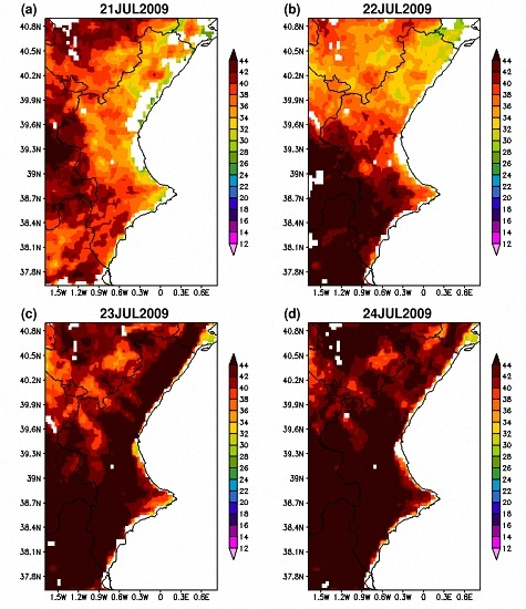
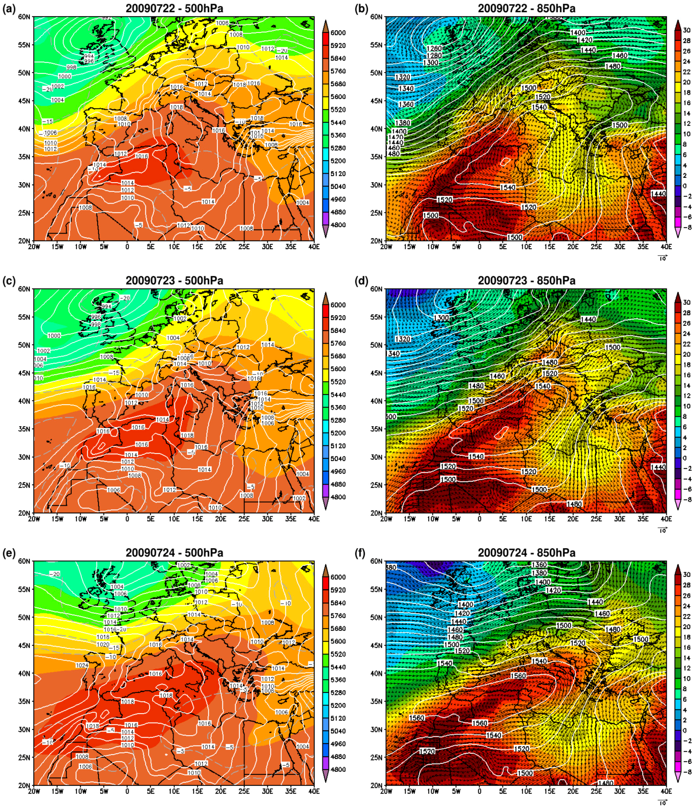
3. Meteorological Description of the Event

During the previous days, the 20 and 21 July, the maximum air temperatures were located over inland areas of the Valencia Province (Figure 1), with values above 30 °C (not shown). On 22 July, the temperature distribution was similar to that found on previous days, but with values around 40 °C in some inland areas, as shown in Table 2 for REQ and PLA, with 38.40 and 39.69 °C, respectively. However, the maximum temperature distribution changed on 23 July, as the higher temperatures moved Easterly to the coast. In this case, values higher than 40 °C were reached not only in typical heat places, such as VNC, with a temperature of 40.79 °C, but also over the Castellón coast, as recorded in CAS and BEN stations, with a maximum temperature of 39.9 and 40.6 °C, respectively (Table 2). The minimum air temperatures were also high within this day, remaining above 20 °C over the coastal strip, as noted by the temperatures reached in ALM and PLA, with 23.16 and 25.92 °C, respectively (Table 3). During the 24 July, temperatures became softened over some areas, such as the Castellón Province, were BEN and CAS recorded 30.5 and 32.5 °C, respectively. Nevertheless, they still recovered and intensified in some locations, reaching once again values near and higher than 40 °C, as reported by the 41.17 and 38.7 °C registered in VNC and CAM, respectively.
The air temperature distribution described in Table 2 and Table 3 is also well reflected in Figure 2, using the SEVIRI-LST product. In terms of maximum temperature, the sea breeze could be developed on 21 and 22 July, thus modulating the observed values, specially the 21 July (not shown). However, Figure 3b shows the advection of South to South-Western warm air to the East coast of Spain, thus producing temperatures around 30 °C at 850 hPa on 22 July. This advection mainly affected the Southern part of the Valencia Region, yielding skin temperatures at 12 UTC higher than 44 °C over Alicante Province and Murcia (Figure 2d). In this case, not only inland areas were influenced by this warm advection, but also these high temperatures reached coastal locations. In addition, this warm advection spread over Valencia Province, but only over inland locations, while the sea-breeze was still able to be developed, thus blocking the entrance of the described synoptic flow (Figure 3b).
On 23 July, this southern advection was displaced to the Mediterranean Sea, while the synoptic flow veered to a marked Western component (Figure 3d) over the Western Mediterranean Coast. Figure 3c shows fair weather over Northern Africa and the Atlantic coast of the Iberian Peninsula joined with a relative low pressure over the Western Mediterranean Basin. This synoptic configuration favoured the development of a Southwestern to Western wind flow towards the Valencia Region (Figure 3d). The SEVIRI-LST product displays very high temperatures at 12 UTC (Figure 2e), essentially influencing the whole region, with the exception of the most onshore sites. In addition, the SEVIRI-LST temperatures present high temperatures on 23 July at 06 UTC (Figure 2b), with values higher than 24 °C over coastal and pre-coastal locations. These elevated temperatures before sunrise were maintained the next day and displaced towards the coast (Figure 2c). In addition, the SEVIRI-LST product reflects a decrease in these temperatures inland in comparison to those observed on 23 July. Considering the synoptic configuration the 24 July, high pressures were established both over the Atlantic and the Mediterranean coasts of the Iberian Peninsula (Figure 3e), with a prevailing anticyclone over the West. This meteorological structure upheld the Western wind circulation over the Western Mediterranean coast (Figure 3f), thus supporting the observed high maximum temperatures (Table 2). This result is also observed using the SEVIRI-LST product, where LSTs higher than 44 °C are extended over the whole Valencia Region (Figure 2f).

4. Results

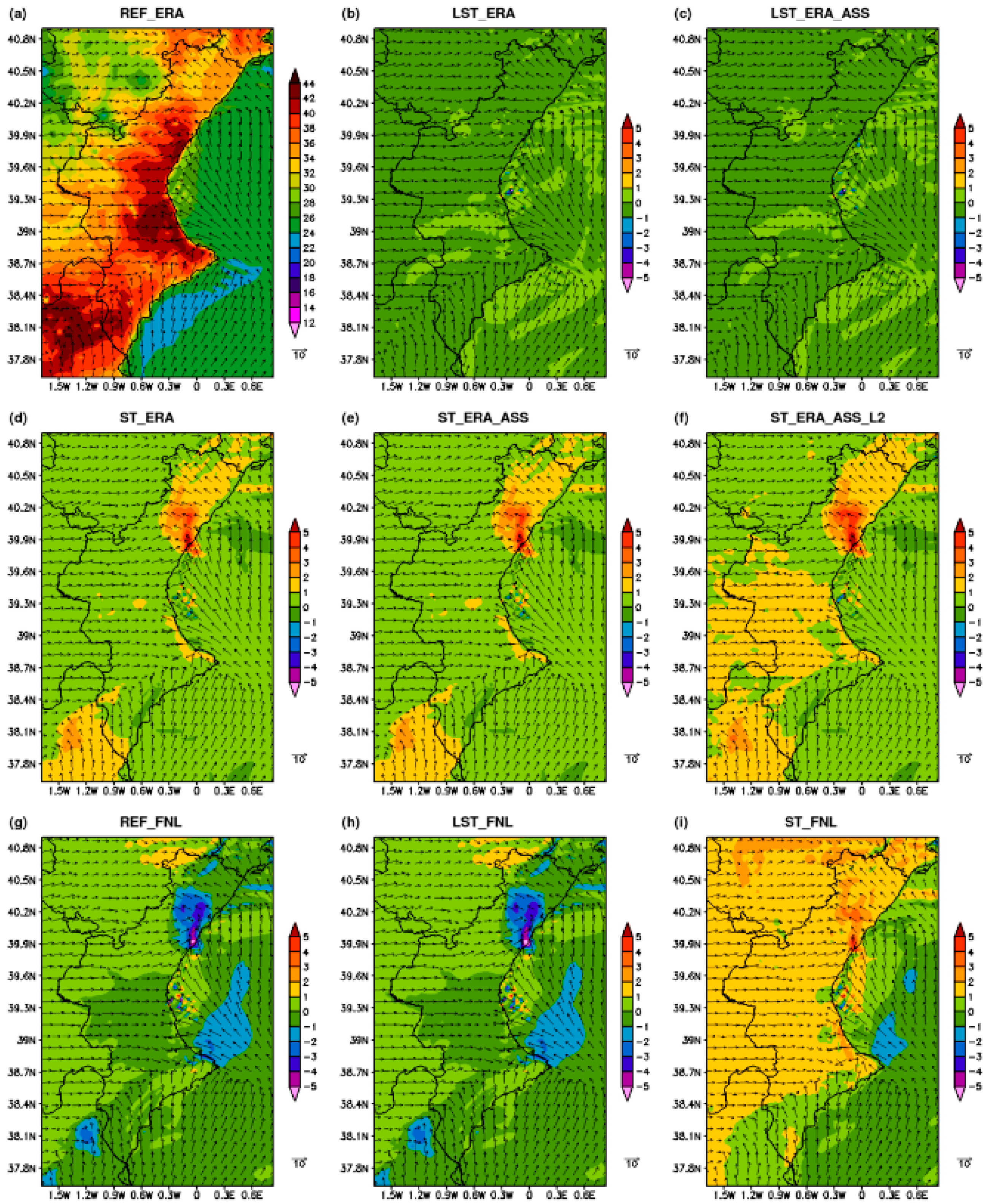
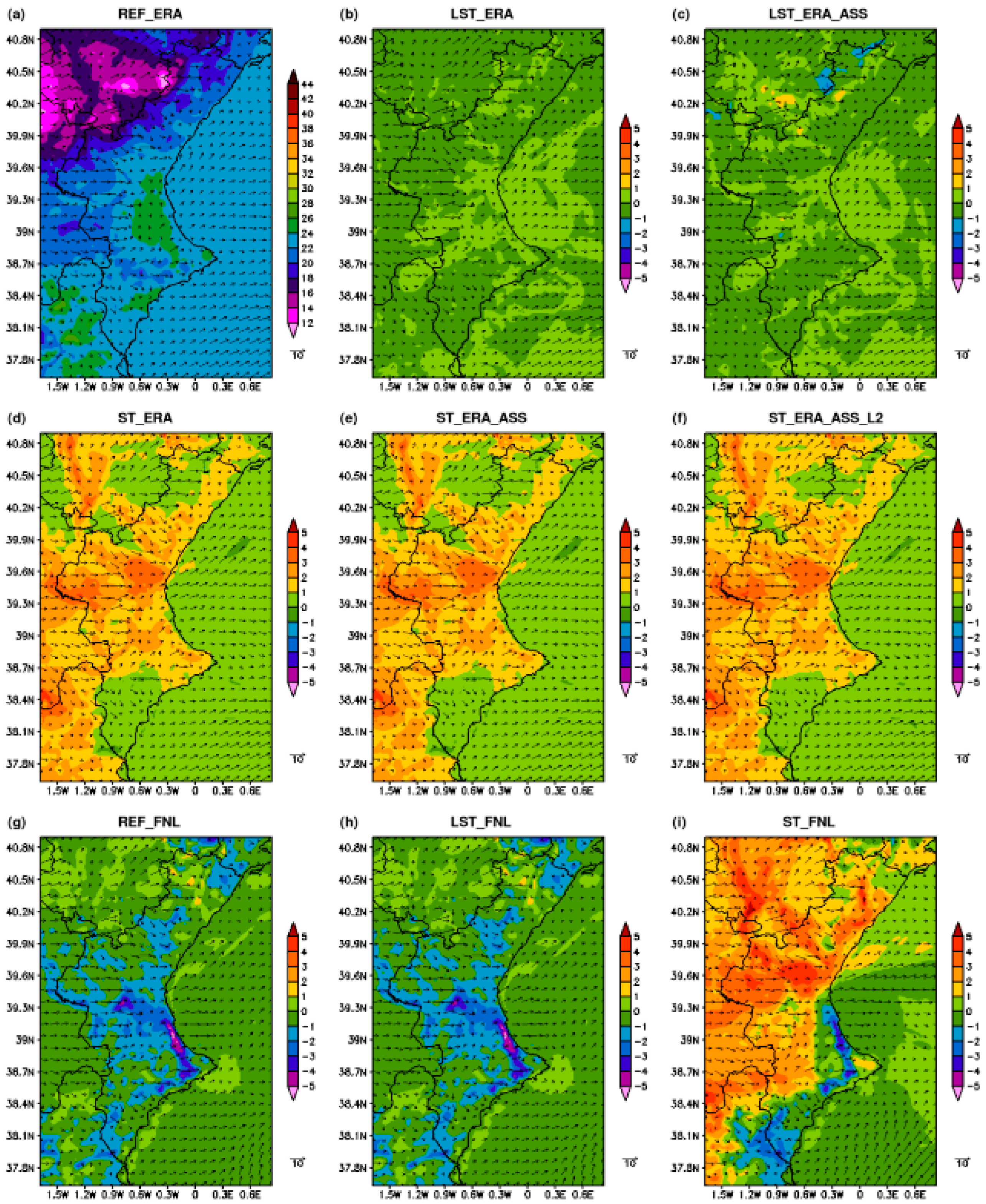
4.1. Daily Maximum and Minimum Temperatures

The statistical scores for the maximum temperature and the different sensitivity experiments have been included in Table 4. Considering the control simulation (REF_ERA), meaningful differences are found for the whole simulation period. The highest errors are obtained on 22 July 2009, with a Bias of 4 °C and an RMSE of 5 °C merging all station data. In this case, both statistical scores slightly increase inland in comparison with the values obtained over coastal locations. In contrast, both the Bias and the RMSE are notably reduced on 23 July. A value of 0.9 °C for the Bias and a RMSE of 3 °C is obtained considering all stations. For this day, the model produces rather accurate results inland, with a Bias of 1.4 °C and RMSE of 2.3 °C. Additionally, considering these sort of stations, a high IoA of 0.8 is reached as well. However, comparing inland with coastal stations, even though the latter shows a lower Bias than the former (0.5 °C), the IoA is considerably lower over coastal sites, indicating that the model has more difficulties in forecasting the maximum temperature pattern observed over coastal locations. Finally, RAMS produces similar results on 24 July inland, but with a negative Bias value of −1.1 °C, indicating that the model has a tendency to underestimate the observations. On the other hand, RAMS reproduces rather well the observations over coastal sites, as shown in the Bias score of −1.2 °C and RMSE of 1.7 °C. Additionally, the IoA in this case is 0.9, indicating that the model properly captures the observed pattern. Considering the Bias score obtained for the control simulation (REF_ERA) merging all stations, the high value of 5 °C obtained on 22 July is reduced to 0.9 °C on 23 July, but still RAMS overestimates the observations. In contrast, this positive trend of RAMS is changed to a negative Bias value of −1.1 °C on 24 July.
Contrasting the results obtained by RAMS for the different initialization datasets, REF_ERA and REF_FNL, no relevant divergences are found in the computed statistical scores, thus the model seems to remain essentially unaffected by the analysis data used in its initialization. In addition, similar results are obtained for the three days of simulation.
Table 4 shows that the use of the LST information derived from analysis and reanalysis datasets, LST_ERA and LST_FNL, has very little or no effect on the 2-m maximum temperature forecasts produced by the control run (REF_ERA). This sensitivity analysis has been carried out for the three days of simulation with the same results and considering both initialization datasets (ERA-Interim and FNL), as it is observed in Figure 4, Figure 5 and Figure 6 for the horizontal structure of the 2-m maximum daily temperature. On the other hand, these figures show that the incorporation of the SEVIRI LST product (LST_ERA_ASS) in the initialization of the model produces little effect in the simulation results as well when compared to those obtained using the LST derived from the reanalysis dataset (LST_ERA).
A different set of experiments have been performed to explore the influence of the ST parameters, including the ST derived from the ERA-Interim and the FNL datasets (ST_ERA and ST_FNL, respectively) in the initial conditions used to start the RAMS simulation. The results obtained show more differences in comparison to the control simulation (REF_ERA) than those obtained using only the LST in the initialization of the model. In general terms, mainly the Bias is reduced for both the 22 and 23 July 2009. For instance, the original Bias obtained on 23 July by REF_ERA (1.4 °C) is reduced to the half using the ST_ERA run (0.7 °C) inland. In contrast, this simulation worsens the accuracy for both inland and coastal stations on 24 July, with a difference of about 0.8 °C between REF_ERA and ST_ERA. In this regard, similar differences are obtained comparing REF_FNL with ST_FNL. Independently of the model deviation from the observations, Table 4 shows that, in all evaluated cases, the introduction of ST derived from reanalysis and analysis data in the initialization conditions, produces lower maximum temperatures than when only the original meteorological datasets are considered or even when only the LST parameter is included in the initial conditions.
Taking into account the ST parameter, two additional experiments have been carried out using the ERA-Interim reanalysis meteorological data together with the LST and ST derived from this model and the satellite-derived LST. Comparing the results obtained by ST_ERA_ASS with ST_ERA rather low differences are obtained for the three days of simulation. Finally, increasing the number of soil levels in the RAMS set-up (ST_ERA_ASS_L2) does not produce a substantial impact on the model results compared to those found using the original soil level distribution and the same LST and ST conditions (ST_ERA_ASS).
Figure 4, Figure 5 and Figure 6 show that the effect of including the ST parameter has a general tendency to produce lower values of the daily 2-m maximum temperature than those simulated by the control run (REF_ERA) and when only the LST is incorporated into the model. Contrasting the FNL with the ERA-Interim results, slight differences are observed for this magnitude.
The results obtained for the minimum temperature from the different sensitivity experiments are presented in Table 5. In this case, the control simulation (REF_ERA) produces substantial differences for the whole simulation period. Thus, considering each day individually, a negative Bias of −0.7 °C and a low value of RMSE of 1.4 °C are reproduced by RAMS on 22 July 2009 merging all stations. However, the tendency of the model is changed on 23 and 24 July, producing an overestimation of the observations, with a value of 2.2 °C and 1.6 °C for the Bias score merging all stations, respectively. Although slight differences are observed in the Bias score contrasting the results obtained over coastal and inland areas on 22 and 23 July, more divergences are found on 24 July, with a difference of 1.1 °C.
As it has been pointed out for the maximum temperature, the minimum temperature results do not show notable differences in relation to the control simulation (REF_ERA) when incorporating the LST to the initial conditions of the simulation. In this regard, using LST information derived from reanalysis (LST_ERA), analysis (LST_FNL) or from the satellite-based product (LST_ERA_ASS) does not produce any significant improvement on the simulation results, and the statistical scores computed for these simulations show similar values as those found for REF_ERA and REF_FNL. Contrasting these latter simulations, it seems that REF_FNL produces worse results concerning minimum temperature than REF_ERA for the three days of simulation.
In contrast, the incorporation of the ST field in the initial conditions using the ERA-Interim meteorological data and the FNL data produces indeed a relevant impact in the simulation results, specially considering the 23 and 24 July 2009. Table 5 shows that the original Bias of 2.1 °C obtained using the control simulation (REF_ERA) on 23 July is reduced to a value 0.2 °C inland. The RMSE of 3 °C reproduced by REF_ERA inland is reduced to 1.8 °C, and the IoA raises from 0.5 to 0.7 comparing both simulations. A similar improvement is found over coastal sites, with a difference of about 1.4 °C in Bias, 1.3 °C in RMSE and 0.2 in IoA comparing REF_ERA with ST_ERA. Furthermore, comparing the influence of the ST field when RAMS is driven by FNL data, a noteworthy improvement is reached using ST_FNL, with a difference of 1.8 °C and about 3 °C in terms of the Bias score on 23 and 24 July merging all stations, respectively. Finally, in the case of the ST simulations, using the LST derived from the SEVIRI sensor (ST_ERA_ASS) does not produce a notable effect when compared to the results obtained using the LST derived from ERA-Interim reanalysis (ST_ERA). The number of soil levels (ST_ERA_ASS_L2) does not report a substantial impact in the simulation of the minimum temperature.
These results are also well reflected in Figure 7, Figure 8 and Figure 9, were it is clear that the usage of the ST parameter is translated into a lowering in the daily minimum temperatures. In addition, it seems that this magnitude is higher when RAMS is initialized using the FNL dataset, compared to the one obtained using ERA-Interim.

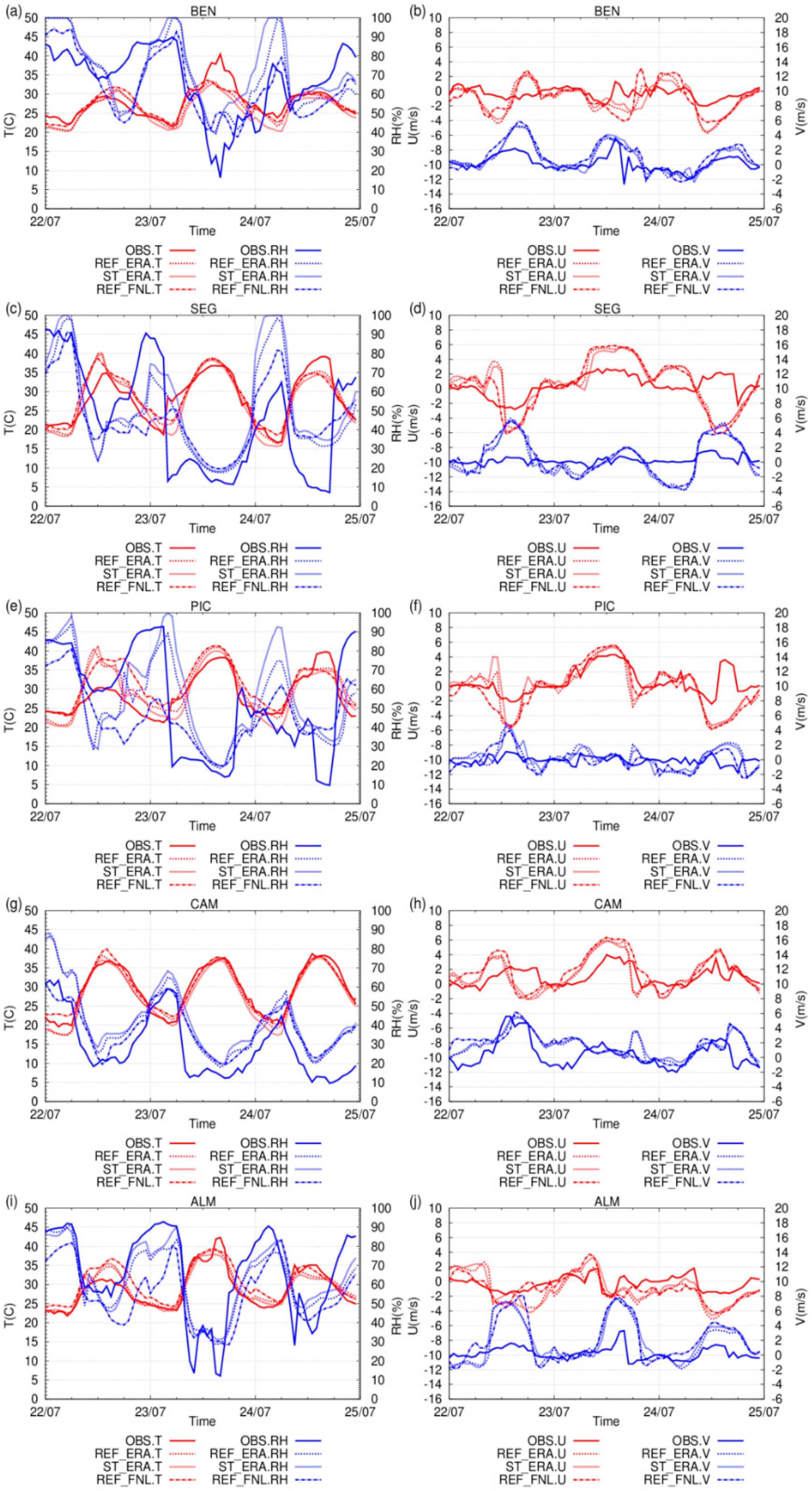
4.2. Wind, Temperature and Moisture Dynamics

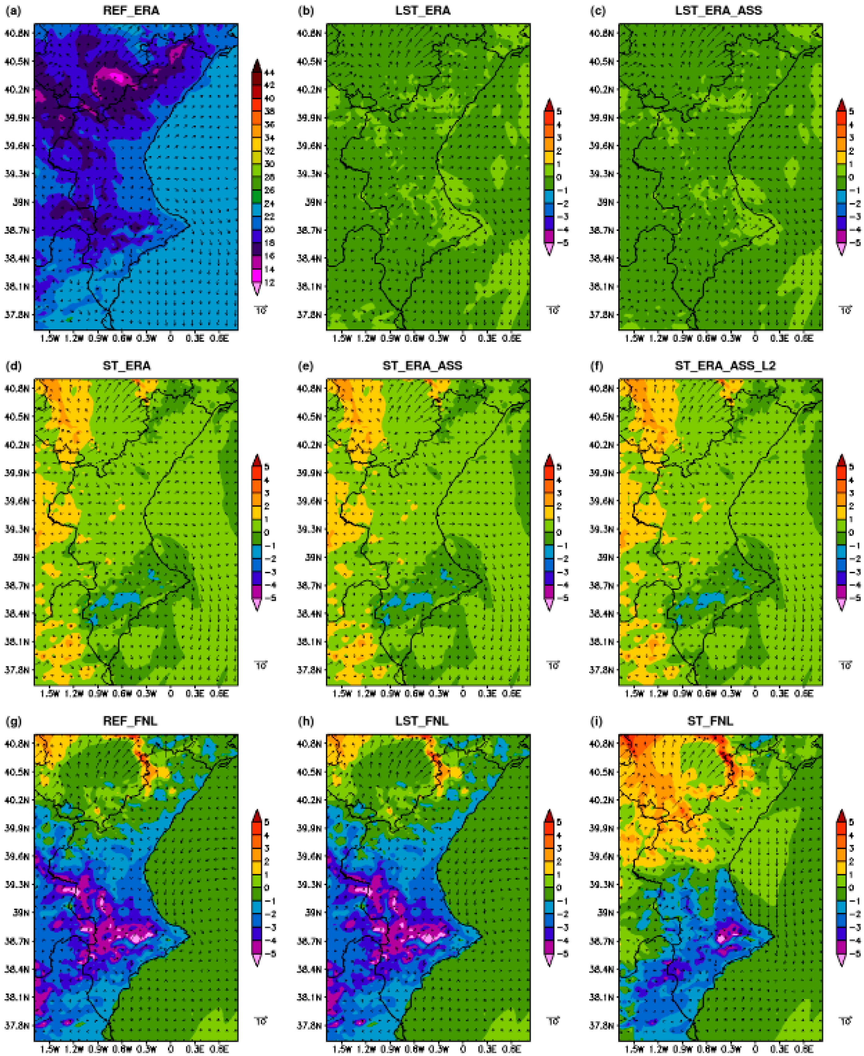
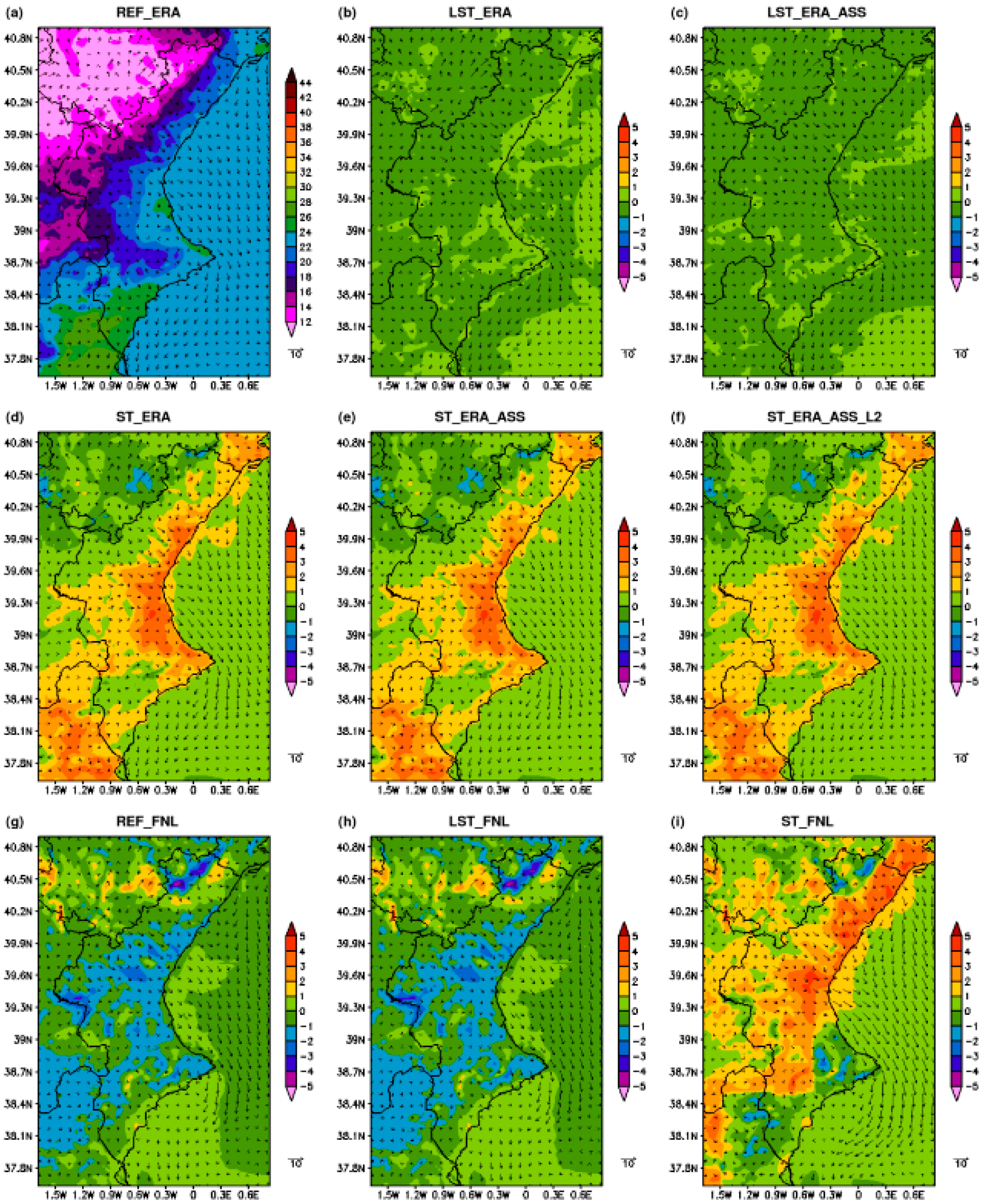
4.2.1. Horizontal Observed and Simulated Patterns

As it has been observed in the previous section, a significant difference has been found among the three days of simulation both for inland and coastal sites in terms of the daily temperature extremes. Considering the case of the maximum temperatures, a positive Bias is found on 22 July (Table 4), which significantly overestimates the observations. However, RAMS reproduces quite well the maximum temperature observed on 23 July inland. Finally, on 24 July, the trend of the model is the opposite as the one found on 22 and 23 July, and RAMS produces a negative Bias, indicating a tendency to underestimate the observations.
In the current section, we focus the analysis on the evolution of the daily temperature (instead of centring the attention in the daily maximum and minimum temperatures), and the relative humidity. Additionally, we try to see the relation between the temperature and the wind field. As can be observed in Figure 4, Figure 5, Figure 6, Figure 7, Figure 8 and Figure 9, the near-surface horizontal wind field remains practically unaffected in relation to the control simulation when using the different LST and ST datasets in the initial conditions of RAMS, both considering the 06 and 15 UTC. In addition, similar results are obtained for the near-surface wind field with all simulations using the same initialization dataset. However, RAMS produces more differences contrasting the ERA-Interim and FNL initialization dataset, even though the general wind flow pattern is rather close in both cases. Considering these results and those obtained in the previous section in terms of maximum and minimum temperatures, we have then focused on the REF_ERA, REF_FNL and ST_ERA experiments, which are those producing the highest divergences among all simulations performed.
Figure 10, shows the hourly evolution of the temperature and relative humidity as well as the eastward and northward wind components, U and V, respectively, considering the weather representative stations of the model behaviour within the area of study. RAMS reproduces the hourly evolution of the temperature in CAM station very well. The maximum temperature is very well captured by the model for the three days of the simulation (Figure 10g). In addition, the minimum temperature is also very captured on 22 July, specially considering the ST_ERA simulation. This RAMS experiment produces lower temperatures than REF_ERA in practically all cases, being the difference between REF_ERA and ST_ERA more marked for the minimum temperatures. Considering the wind components over CAM station, Figure 10h shows that the model reproduces the wind pattern properly.
If we focus on PIC station, there is a significant overestimation of the simulated maximum temperature on 22 July (Figure 10e). In this case, there is clear modelled Westerly flow for the first hours of the day nearly until noon. From this time on, the model establishes a see breeze circulation that is maintained the rest of the day (Figure 10f). However, the observations show that this sea breeze actually started earlier, thus modulating the observed maximum temperature and not permitting to reach the high temperatures produced by RAMS for this day. Comparing the 22 with the 23 July, even though the model still overestimates the observed temperatures, there is a better agreement on 23 July. In this case, both RAMS and the observations present a clear Westerly flow that is the responsible for the high temperatures produced this day, with a value of 38.3 °C in PIC (Table 2). In contrast, on 24 July, the model shows the opposite trend as that obtained the previous days, thus underestimating the observations, as it has already been shown in the previous section. PIC station perfectly illustrates this situation, in which both the model and the observations reproduce a sea breeze circulation that is started early in the morning. In this case, the temperature is modulated, as it is observed in Figure 10e. However, even though the model continues with this sea breeze flow thus maintaining the temperatures away from reaching higher values, the observations show a shift in the wind direction (Figure 10f) around noon. From this time on, the wind veers to a Westerly flow that produces the temperatures to recover and reach higher temperatures, of 39.8 °C (Table 2). This same pattern is observed in SEG station (Figure 10d), although the observed western flow is initiated earlier than in PIC (Figure 10d). As a result of this delay in the wind veering, the temperatures are still able to recover (Figure 10c,e).
Finally, the same behaviour found in PIC on 22 July has also been found in ALM, but with a less divergence of the model in relation to the observations. In this regard, Figure 10j shows how the observations start the sea breeze flow earlier than the model, thus modulating the maximum temperature (Figure 10i).
The wind and temperature dynamics of this episode show a different behaviour of the model depending on its ability to reproduce the interface between the sea breeze circulation and the Westerly flow. In this regard, the 22 July is an example that illustrates the case where the model continues a westerly flow while the observations allow an early development of the sea breeze. RAMS maintains the former flow more time than observed for this day, thus producing a substantial increase in temperature that is uphold even though the sea breeze circulation starts at about noon. The heterogeneous distribution of the interface between these two divergent meteorological conditions produces a relevant overestimation of the maximum temperature, as it has been seen in the previous section. In contrast, the 23 July is an example of a day where a more homogeneous atmospheric condition is established over the whole region, and where the Westerly wind flow dominates. As a result, RAMS reproduces the observations in a better way and the difference between the model and the observations is notable reduced compared to the divergences obtained the previous day. In this case, the maximum deviation of the model in relation to the observations is obtained in the coastal stations over Castellón Province, where the model favours a sea breeze development while the observations show a Westerly flow reaching coastal areas. This behaviour is illustrated in Figure 10b, where the observations as well as the model show the initiation of the sea breeze, which mitigates the level of temperature in the early morning (Figure 10a). This sea breeze is preserved by the model, thus modulating the maximum temperatures. In this case, RAMS produces maximum temperatures around 33 °C in BEN station. However, the observed wind flow changes from this sea breeze to a Westerly flow permitting the temperatures to immediately recover, reaching very high values (40.6 °C) over the coast of Castellón Province (Figure 10a). This disagreement between the model and the observations is the responsible for the higher errors obtained this day when considering coastal sites, where for instance the IoA is notably reduced compared to the one obtained over inland locations (Table 4).
The described wind patterns are well represented in the relative humidity as well at all stations. For instance, a very low relative humidity (below 10%) is observed on 23 July in BEN and SEG stations (Figure 10a,c), during the day time and under the Western synoptic forcing, in contrast to those values of relative humidity, around 70%, in BEN the previous day under the influence of the sea breeze. At all stations, the transition between the different wind circulations is clear. In contrast, a really low relative humidity is observed over CAM for the three days of simulation (below 10%), where a Western synoptic advection was well-established and rather high temperatures were recorded (Figure 10g). In this case, the model shows a tendency to slightly overestimate the measurements. Nevertheless, over CAM station, the model reproduces really well the maximum temperatures observed, as shown in Figure 10g as well as in Figure 4, Figure 5 and Figure 6.
Finally, comparing the results provided by REF_ERA, ST_ERA and REF_FNL, it is observed that the latter produces in general the highest temperatures and the lowest relative humidity, with REF_ERA and ST_ERA being more alike. In these terms, these two simulations are more comparable for the horizontal wind components, with REF_FNL presenting more divergences in relation to REF_ERA and ST_ERA, as can also be seen in Figure 4, Figure 5, Figure 6, Figure 7, Figure 8 and Figure 9 for the near-surface wind field.

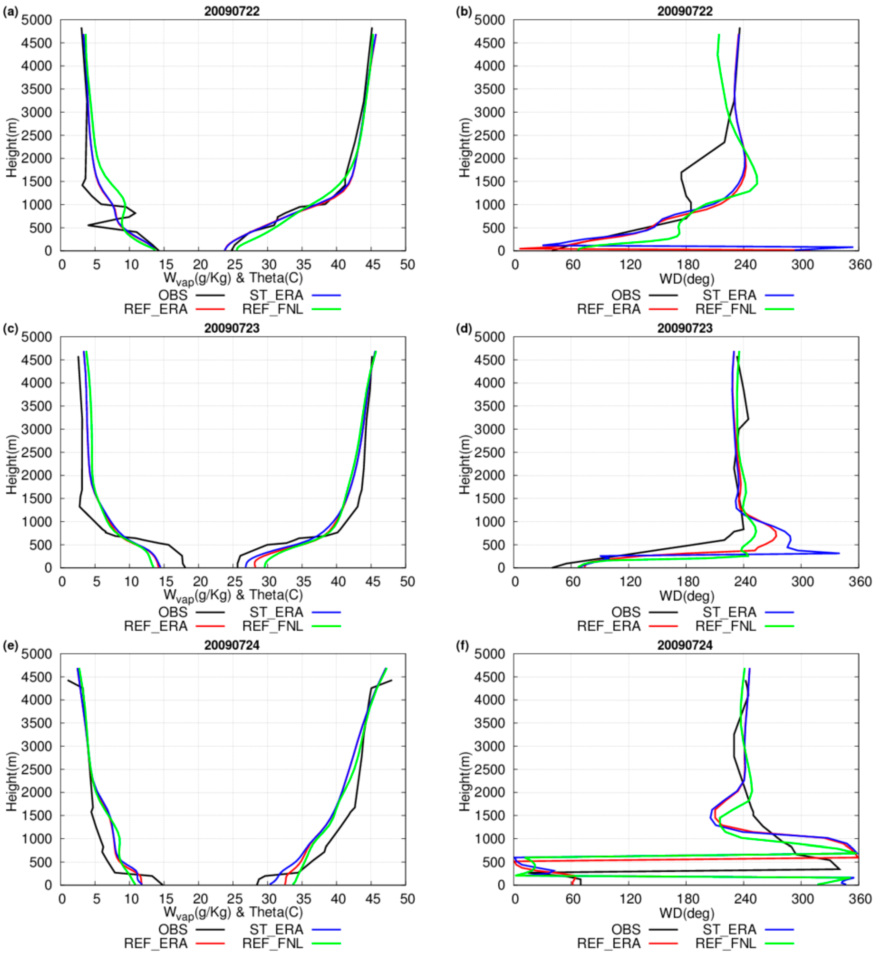
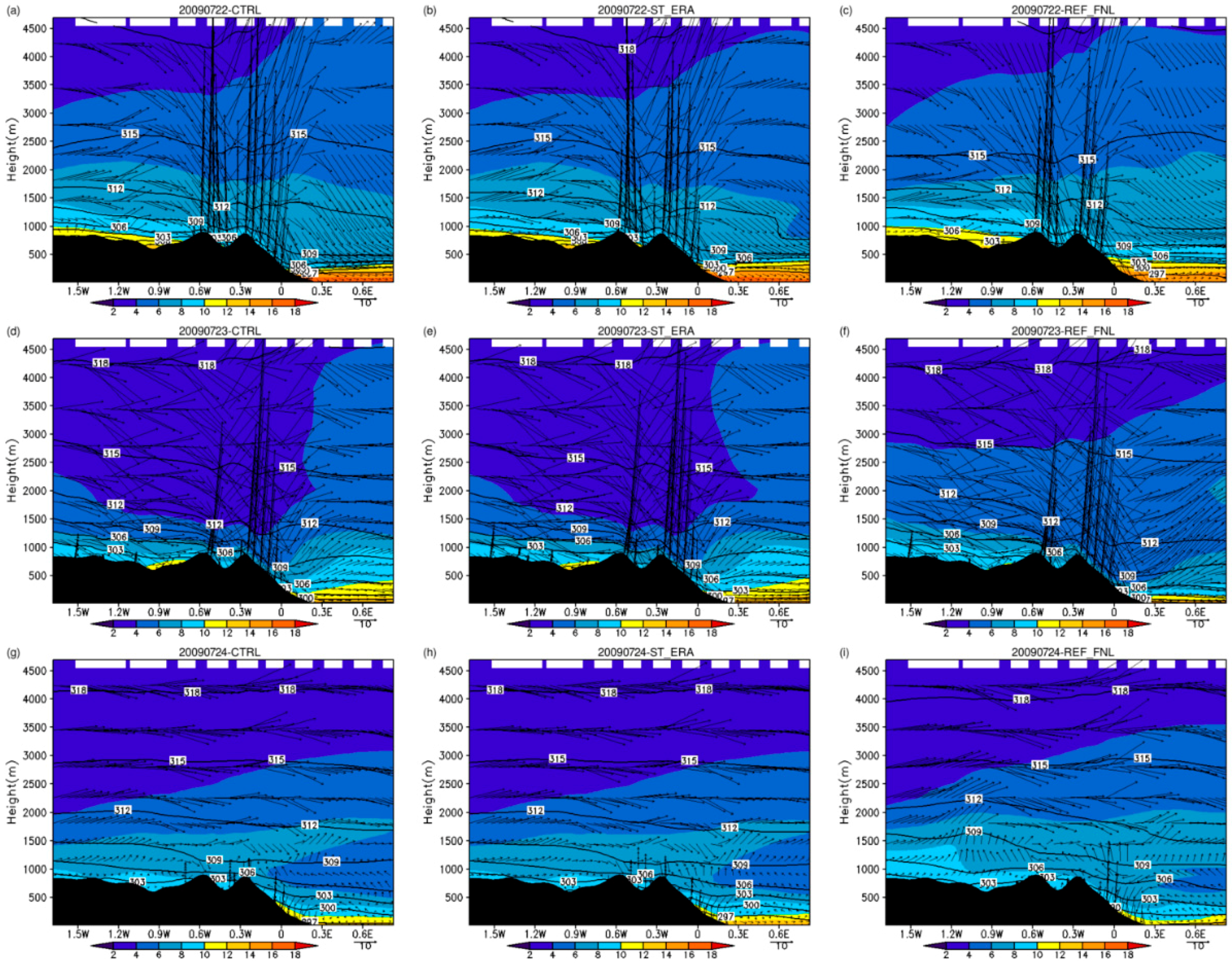
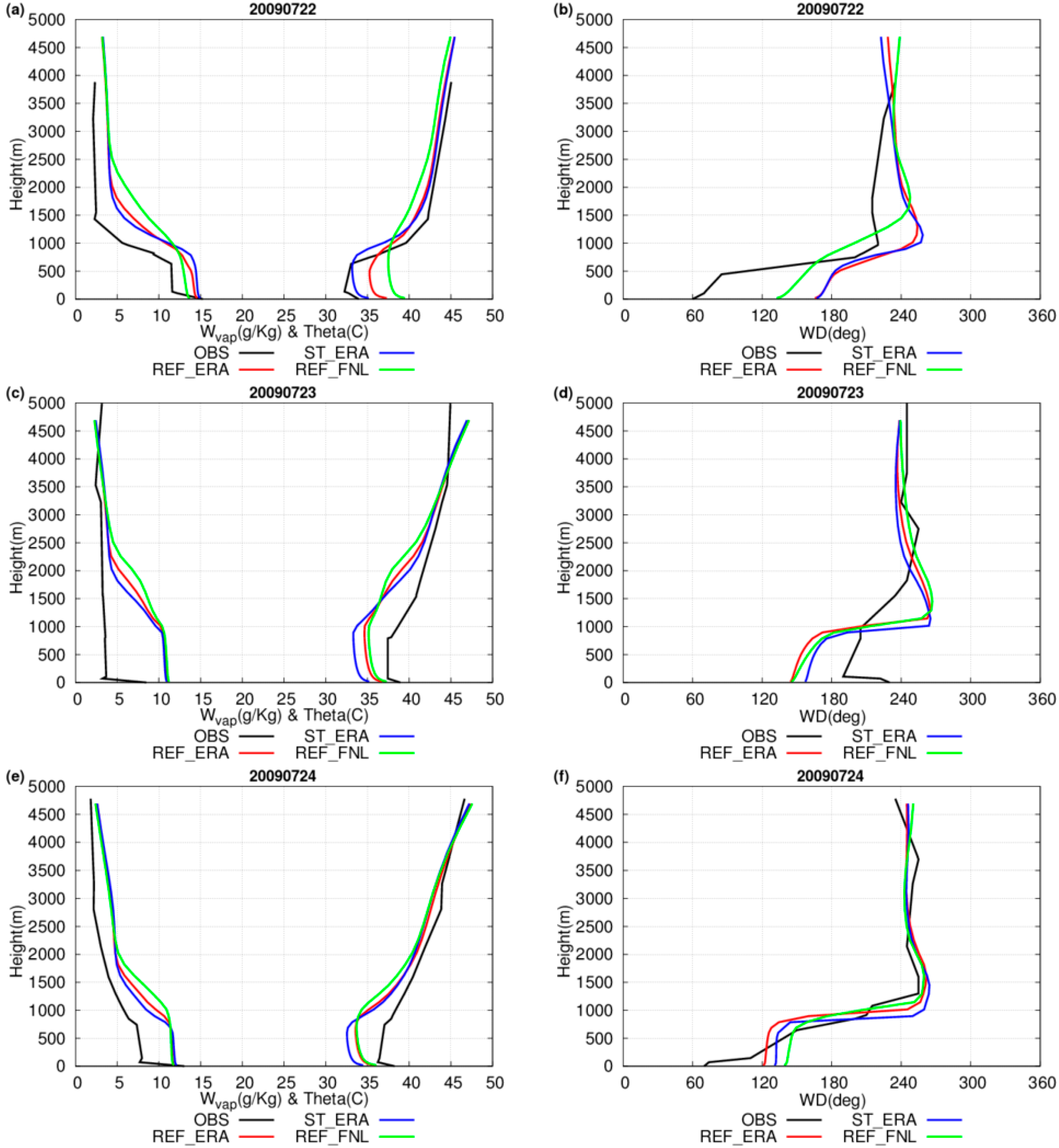
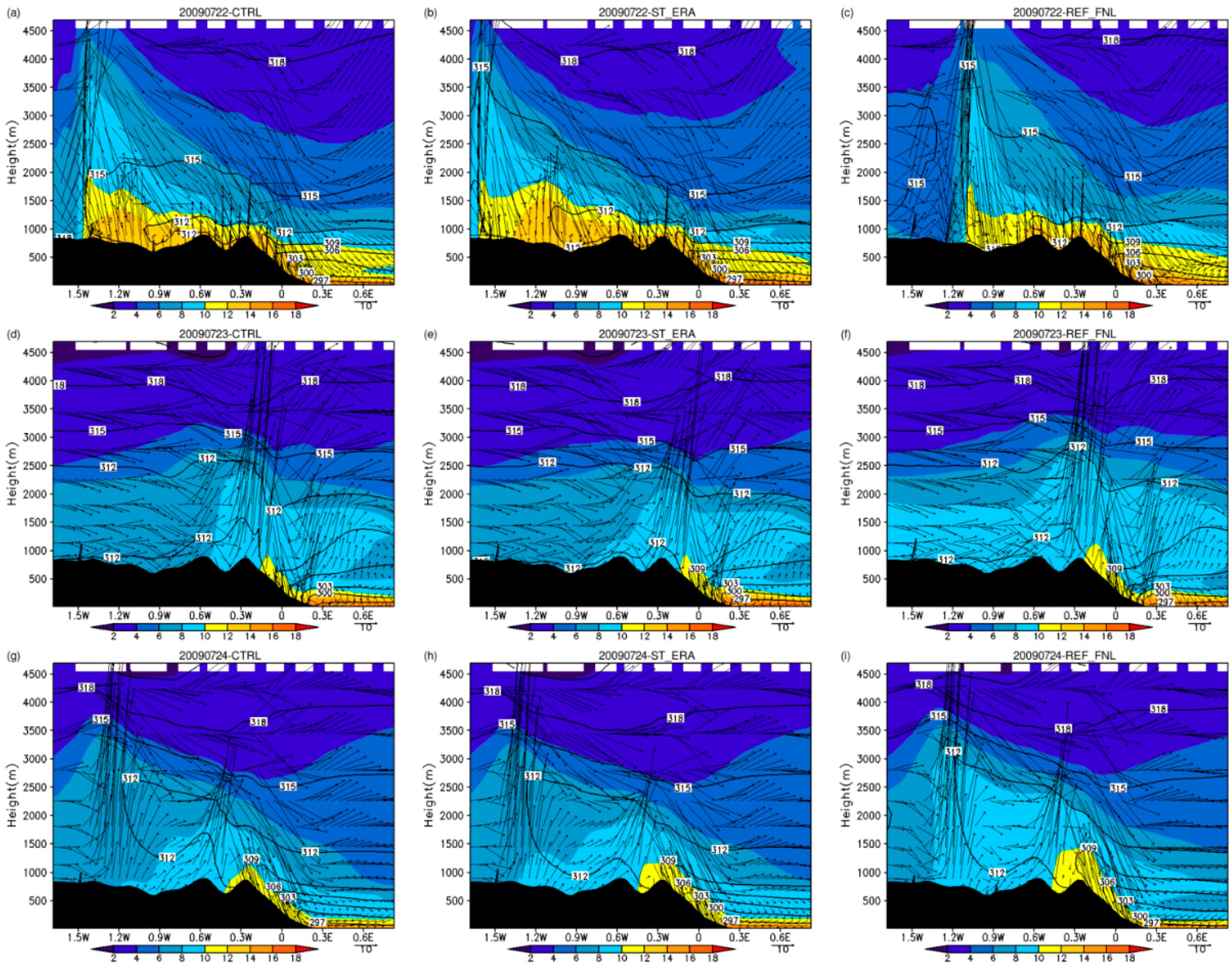
4.2.2. Vertical Observed and Simulated Patterns

The upper air model results are compared with the MUR sounding (Figure 1) for the REF_ERA, ST_ERA and REF_FNL simulations, considering the 00 UTC (Figure 11) sounding on 22–24 July 2009. In terms of the water vapor mixing ratio, values around 15 g/kg are found near the surface, while this magnitude decreases rapidly with height to values below 5 g/kg above 500 m. Considering the measurements on 22 July, the model reproduces really well both the vertical moisture and the potential temperature, with the ERA simulations closer to the observations (Figure 11a). Comparing the observations for this day with those recorded on 23 July and 24 July, some meaningful differences are obtained in the vertical distribution of this meteorological variable. On 23 July, a fast and marked decrease in the vertical moisture is found at about 500 m height in the first case (Figure 11c) and below 500 m height in the second case (Figure 11e), yielding a drop of around 10 g/kg within a reduced layer. Comparing RAMS with the observations, the model reproduces the observed vertical moisture pattern, but with a smoother transition on 23 July, while this vertical shift is less clear on 24 July. In any case, this same model trend is seen in relation to the measurements on both days, underestimating the near surface values while they are slightly overestimated upwards.
On the other hand, the same transition observed in the vertical moisture is obtained in the vertical potential temperature. In this regard, an increase of approximately 20 °C is found on 23 July within the 500–1000 m layer, with a raise in temperature of about 15 °C in just 400 m (Figure 11c). The same behaviour is observed on 24 July (Figure 11e), but not as marked as on 23 July. In this latter case, RAMS captures the main patterns observed. However, as in the case of the vertical moisture, the modelled transition between the low near surface temperatures and the high upper level temperatures is smoother than in the measurements. In contrast, the model does not reproduce the observed transition of these magnitudes between near surface and upper levels on 24 July, yielding a more constant increase in the vertical variation of the potential temperature, and a decrease in the case of the water mixing ratio.
Comparing REF_ERA, ST_ERA and REF_FNL, the latter produces the highest temperatures, while ST_ERA shows the lowest ones near the surface. However, these divergences among the different simulations are reduced in upper levels, where the model shows an underestimation of the measurements. The introduction of the ST parameter seems to better reproduce the vertical potential temperature near the surface. The tendency of the model in relation to the observations is just the opposite in terms of the vertical moisture, where the model underestimates the measurements near the surface while they are overestimated upwards.
Considering the wind flow at 00 UTC, a North-Eastern wind flow is observed the three days of simulation over and near the surface (Figure 11). However, this wind field veers to a marked Western synoptic circulation aloft, specially on 23 July, where this flow is already established below 1000 m (Figure 11d). Contrasting the measurements with the model, RAMS reproduces very well the observed wind field both near the surface and aloft.
These results found over MUR are supported by Figure 12 for a vertical cross section at 38.7°N and at 06 UTC, over a geographical area where RAMS reproduces very well the observations within the whole simulation period (Figure 10). This figure presents the vertical distribution of the potential temperature, water vapor maxing ratio and wind field. In general, there is a Western wind flow in the whole vertical layer for all days, although some differences have been found among them. In this regard, on 22 and 23 July 2009, a relevant downward motion is simulated by RAMS over coastal and pre-coastal areas (Figure 12a,d). In addition, the geographical barriers provoke an upward flow due to the convergence simulated towards the coast. On the other hand, on 24 July a more stable weather is found at night (Figure 12g). Comparing REF_ERA with ST_ERA and REF_FNL, rather similar results are found at night considering the three days of simulation.
Figure 13 presents the observed MUR sounding and RAMS-simulated vertical structure of the potential temperature, water vapor mixing ratio and wind direction for the three days of simulation at 12 UTC. On 22 July (Figure 13a), high moisture content, about 15 g/kg, is observed near the surface, decreasing to values of about 3 g/kg below 1500 m, with a reduction of approximately 10 g/kg within the 500–1500 m layer. The same pattern is simulated by RAMS, thus rather well capturing the observations. However, a notable change in the moisture content was recorded within the lowest layer near the surface. On 23 July (Figure 13c), the moisture content is substantially reduced compared to the values found the previous days. In this regard, a fast reduction is observed in this magnitude very near the ground, within a height lower than 100 m, starting from a value lower than 10 g/kg and reaching a value lower than 5 g/kg, which is maintained nearly constant with height. In this case, RAMS produces high moisture content within the lowest 1000 m, higher than 10 g/kg, thus clearly overestimating the observations. Finally, on 24 July (Figure 13e), the vertical distribution of the moisture content shows an intermediate situation between the one found on 22 and the one found on 23 July, with a smoother decrease of this magnitude with height, except in those layers very close to the ground.
Comparing the observations with the model, RAMS tends to overestimate them, specially on 23 July. However, even though this overestimation is reproduced on 22 and 24 July as well, it is considerably reduced, particularly on 22 July. The model captures the observed pattern properly both on 22 and 24 July, but with larger values than observed very near the ground. In this sense, RAMS simulates a nearly constant moisture content in the lowest troposphere.
The results obtained for the moisture content are translated to the potential temperature. In this regard, a lower mixing layer height is observed on 22 July, lower than 1000 m (Figure 13a). However, the vertical inversion observed on this day between 500 and 1000 m is broken on 23 and 24 July (Figure 13c,e), and just a very small inversion is maintained. On the other hand, even though RAMS captures rather well the observations on 22 July, the model underestimates the measured potential temperature on 23 and 24 July, developing a significant inversion layer in contrast to the observations.
Comparing the different RAMS simulations, in general REF_FNL produces higher temperatures than REF_ERA and ST_ERA in the lowest troposphere, especially on 22 July, more dominated by the development of sea breezes. In addition, REF_FNL enhances the mixing layer height in comparison both with the observations and the other RAMS simulations. In this regard, contrasting REF_ERA and ST_ERA, it is found (Figure 13) that incorporating the ST field in the model produces in general lower temperatures not only in the surface, as shown in previous sections, but also in the vertical within the lower troposphere. In addition, this parameter produces a slight reduction in the mixing layer height in comparison to the height obtained using REF_ERA.
The observed wind direction shows a similar vertical structure on 22 and 24 July, where it veers from a Northeasterly flow over the surface to a Southwesterly circulation in upper levels. The latter is well established as the vertical wind configuration on 23 July. Although RAMS reproduces the observed wind structure aloft, it shows a tendency to produce a Southeasterly wind field near the surface for the three days of simulation. This seems to be the reason of the differences found between the model and the observations in terms of the water vapor mixing ratio and the potential temperature. Thus, an advection from the sea, as simulated by RAMS produces an increase in the moisture content and a decrease in the temperature, while a more marked Westerly wind flow is translated in a decrease in the moisture content and an increase in temperature. This result is clearer on 23 July (Figure 13c,d), where the synoptic configuration produces a Western advection of warm and dry air over MUR station. The vertical structure of the evaluated parameters is also well supported by the near surface observations recorded (not shown) in MUR station, where on 22 July, a 2-m maximum temperature of 39.2 °C was reached, with a North-Easterly wind flow and a relative humidity near 30% at day time. Similar measurements were recorded on 24 July, with a 2-m maximum temperature of 39.4 °C. In contrast, a marked Southwesterly wind flow is observed on 23 July, producing a very high temperature (44.4 °C) and low relative humidity (9%) at 15 UTC.
These results found over MUR are also well represented in Figure 14 for the vertical cross section at 38.7°N. This figure presents the vertical structure of the potential temperature, as well as the moisture content and the wind field, as simulated by the RAMS model at 15 UTC for the three days of simulation. In this regard, a Westerly wind flow is established over this area, favouring an advection of dry and warm air towards the coast, where it is partially blocked by the development of a sea-breeze circulation very near the coast (Figure 14d). The convergence of a these two wind patterns produces an important vertical ascent above the first coastal orographic barriers as well as a downward motion of the air onshore, both on 23 and on 24 July (Figure 14d,g). However, this convergence line is displaced inland in the second case, as the sea-breeze is able to reach more inland areas (Figure 14g). This result is reproduced by the vertical distribution of the water vapor mixing ratio as well. Focused on 22 July (Figure 14a), the progress of the sea-breeze towards inland areas also produces this convergence line. In this regard, the moisture content is able to move in the direction of these areas, showing a boundary between the sea-breeze circulation and the Western synoptic advection, which is limited to the most inland sites in comparison to the location of this boundary on 23 and 24 July 2009. Finally, comparing the results produced by REF_ERA, ST_ERA and REF_FNL in terms of the variables analysed, a similar pattern is simulated by RAMS, with slight differences among them. In this case, the greatest differences are observed on 22 July, when the Western synoptic advection is displaced by REF_FNL to the coast in contrast to REF_ERA and ST_ERA, thus displacing the location of the mentioned convergence line. Contrasting REF_ERA and ST_ERA, it seems that the latter permits the sea-breeze to slightly move inland.

5. Conclusions

The current work focuses on the study of an extreme heat weather event that took place between the 22 and 24 July 2009, which resulted in high temperatures over the coastal Valencia Region. This episode recorded maximum temperatures higher than 40 °C amply extended over this region as well as minimum temperatures easily exceeding the threshold of 20 °C, and reaching values up to 25.92 °C. Among these three days, the 23 July was characterized by a dominant and widely extended Western synoptic advection, while on the 22 and 24 July this atmospheric situation dominates inland but a sea-breeze develops onshore. In this case, this mesoscale circulation is able to reach inland areas as the day progresses, thus converging with the Western advection.
The results obtained in the simulations indicate a diverse model skill depending on its ability to reproduce the boundary where the convergence of these two opposite flows is located. In this regard, the maximum temperatures are really well captured on 23 July, where this Western advection is more extended over the region of study. The model presents more difficulties over the Castellón coastal region (Figure 1), where it is not able to capture the observed Western advection. In contrast, the model overestimates the observations on 22 July, with high statistical scores. The temperature and wind dynamics have revealed that RAMS promotes the development of a Western advection towards the coast, while this wind flow was in fact maintained inland. We find the opposite trend on 24 July, where the model develops a marked sea-breeze that is supported by the observations, but a veering of the observed wind from this sea-breeze to a Western advection produced a recovery of the recorded maximum temperatures. As a result, RAMS underestimates the observations in this case.
Therefore, RAMS is able to properly capture the observed patterns in those cases where a Western advection is widely extended over the area of study (23 July). The orographic configuration as well as the geographical and physical features of the region of study (Figure 1), provokes the convergence of two opposite wind flows, a Western synoptic advection and a sea-breeze circulation, as it is clear for the 22 and 24 July. Thus, the RAMS skill in those cases where a sea-breeze is well developed depends on the proper location of the boundary of this convergence line. These results highlight the difficulties that appear in a coastal area, such as the Valencia Region, due to these convergent flows, and it is an important issue that should be carefully considered in the forecast of these sort of atmospheric frameworks over these areas.
The main motivation for the current study originated in considering the tendencies of the maximum and minimum temperatures simulated by the original operational weather forecasting system implemented over the area of study [35,39]. For that reason, and in order to evaluate the impact of different physical and atmospheric related processes and feedbacks in the simulation results, different sensitivity tests have been performed. Firstly, two different input data sources have been used to drive RAMS: FNL and ERA-Interim datasets. In general, both datasets show a similar skill of RAMS. However, ERA-Interim simulations present a better agreement with the observations in relation to those performed using FNL. Secondly, we examine the role of improved initial LST and ST parameters on the simulation results by means of modelling and satellite-derived products. Using the LST field as a parameter to create the initial conditions of the model does not present a relevant influence on the results of both maximum and minimum temperatures. Indeed, the use of the LST product derived from the MSG-SEVIRI data, with a much more detailed horizontal spatial resolution than that derived from ERA-Interim or FNL, does not produce a notable influence. The inclusion of this parameter derived from these different dataset sources shows practically the same results that the control simulation. These results agree with those found by [60], where the use of improved initial conditions of LST provided within the MM5 mesoscale model by the Moderate Resolution Imaging Spectroradiometer (MODIS) Terra and Aqua satellites, had a positive impact on the model skill to reproduce the 2-m temperature only during the first 9 h of the simulation, but this impact almost vanished later on. It is worth noting here that a spin-up of 12-h has been chosen in the design of the present RAMS simulations.
To see a more marked impact on the simulation results, it is necessary to consider the ST field obtained for different soil levels. In this regard, those simulations that take into account this magnitude show a relevant difference in relation to the control run. Additionally, in all cases, the incorporation of the ST field in the initial conditions shows a tendency to produce lower temperatures than those simulated by the control run. Finally, once used the ST field as a bottom initial condition for RAMS, increasing the number of soil levels to spread deeper underground (13 levels with a soil depth of 1.5 m) does not produce any meaningful impact on the simulation results, which are essentially the same as those found only using the original soil levels distribution (11 levels with a soil depth of 0.5 m).

Acknowledgments

This work has been funded by the Spanish Ministerio de Economía y Competitividad and the European Regional Development Fund (FEDER) through the project CGL2015-64268-R (MINECO/FEDER, UE), by the Regional Government of Valencia through the project PROMETEOII/2014/086 and by the Spanish Ministerio de Economía y Competitividad through the project CGL2011-30433-C02-02 (MINECO). NCEP is acknowledged for providing the FNL analysis data for RAMS initialization. ECMWF and Land Surface Analysis Satellite Application Facility (LSA SAF) are acknowledged as well for providing the ERA-Interim reanalysis dataand the satellite data, respectively. Additionally, the authors acknowledge the Atmospheric Soundings portal of the University of Wyoming for providing the radiosonde data. We would also like to thank the Spanish Ministry of Agriculture, Food and Environment for making the surface observations available through the SIAR system. Finally, the authors want to thank the valuable and detailed reviewers’ comments.

Author Contributions

Igor Gómez and Vicente Caselles conceived and designed the experiments; Igor Gómez performed the experiments; Igor Gómez and Raquel Niclòs analyzed the data; Vicente Caselles and María José Estrela contributed reagents/materials/analysis tools; Igor Gómez and María José Estrela wrote the paper.

Conflicts of Interest

The authors declare no conflict of interest.

References

  1. IPCC. Climate Change 2014: Impacts, Adaptation and Vulnerability; Working Group II Contribution to the Intergovernmental Panel on Climate Change Fifth Assessment Report (WGII AR5) 2014; Summary for Policymakers (SPM); IPCC: Geneva, Switzerland, 2014. [Google Scholar]
  2. Easterling, D.R. Maximum and minimum temperature trends for the globe. Science 1997, 277, 364–367. [Google Scholar] [CrossRef]
  3. Easterling, D.R.; Meehl, G.A.; Parmesan, C.; Changnon, S.A.; Karl, T.R.; Mearns, L.O. Climate extremes: Observations, modeling, and impacts. Science 2000, 289, 2068–2074. [Google Scholar] [CrossRef] [PubMed]
  4. Miró, J.J.; Estrela, M.J.; Millán, M. Summer temperature trends in a Mediterranean area (Valencia Region). Int. J. Climatol. 2006, 26, 1051–1073. [Google Scholar] [CrossRef]
  5. Della-Marta, P.M.; Haylock, M.R.; Luterbacher, J.; Wanner, H. Doubled length of Western European summer heat waves since 1880. J. Geophys. Res. 2007. [Google Scholar] [CrossRef]
  6. Stéfanon, M.; Drobinski, P.; D’Andrea, F.; Lebeaupin-Brossier, C.; Bastin, S. Soil moisture-temperature feedbacks at meso-scale during summer heat waves over Western Europe. Clim. Dyn. 2013, 42, 1309–1324. [Google Scholar] [CrossRef]
  7. Miró, J.; Estrela, M.J.; Olcina-Cantos, J. Statistical downscaling and attribution of air temperature change patterns in the Valencia region (1948–2011). Atmos. Res. 2015, 156, 189–212. [Google Scholar] [CrossRef]
  8. Fischer, E.M.; Schär, C. Consistent geographical patterns of changes in high-impact European heatwaves. Nat. Geosci. 2010, 3, 398–403. [Google Scholar] [CrossRef]
  9. El Kenawy, A.; López-Moreno, J.I.; Vicente-Serrano, S.M. Recent trends in daily temperature extremes over northeastern Spain (1960–2006). Nat. Hazards Earth Syst. 2011, 11, 2583–2603. [Google Scholar] [CrossRef] [Green Version]
  10. El Kenawy, A.; López-Moreno, J.I.; Vicente-Serrano, S.M. Trend and variability of surface air temperature in northeastern Spain (1920–2006): Linkage to atmospheric circulation. Atmos. Res. 2012, 106, 159–180. [Google Scholar] [CrossRef]
  11. Fernández-Montes, S.; Rodrigo, F.S. Trends in seasonal indices of daily temperature extremes in the Iberian Peninsula, 1929–2005. Int. J. Climatol. 2012, 32, 2320–2332. [Google Scholar] [CrossRef]
  12. Acero, F.J.; García, J.A.; Gallego, M.C.; Parey, S.; Dacunha-Castelle, D. Trends in summer extreme temperatures over the Iberian Peninsula using nonurban station data. J. Geophys. Res. Atmos. 2014, 119, 39–53. [Google Scholar] [CrossRef]
  13. Fonseca, D.; Carvalho, M.J.; Marta-Almeida, M.; Melo-Gonçalves, P.; Rocha, A. Recent trends of extreme temperature indices for the Iberian Peninsula. Phys. Chem. Earth 2015. [Google Scholar] [CrossRef]
  14. Fischer, E.M.; Seneviratne, S.I.; Lüthi, D.; Schär, C. Contribution of land-atmosphere coupling to recent European summer heat waves. Geophys. Res. Lett. 2007. [Google Scholar] [CrossRef]
  15. Fischer, E.M.; Seneviratne, S.I.; Vidale, P.L.; Lüthi, D.; Schär, C. Soil moisture-atmosphere interactions during the 2003 European summer heat wave. J. Clim. 2007, 20, 5081–5099. [Google Scholar] [CrossRef]
  16. Teuling, A.J.; Seneviratne, S.I.; Stäckli, R.; Reichstein, M.; Moors, E.; Ciais, P.; Luyssaert, S.; van den Hurk, B.; Ammann, C.; Bernhofer, C.; et al. Contrasting response of European forest and grassland energy exchange to heatwaves. Nat. Geosci. 2010, 3, 722–727. [Google Scholar] [CrossRef]
  17. Stéfanon, M.; D’Andrea, F.; Drobinski, P. Heatwave classification over Europe and the Mediterranean region. Environ. Res. Lett. 2012. [Google Scholar] [CrossRef] [Green Version]
  18. Stéfanon, M.; Drobinski, P.; D’Andrea, F.; Noblet-Ducoudré, N. Effects of interactive vegetation phenology on the 2003 summer heat waves. J. Geophys. Res. Atmos. 2012. [Google Scholar] [CrossRef]
  19. Dasari, H.P.; Salgado, R.; Perdigao, J.; Challa, V.S. A regional climate simulation study using WRF-ARW model over Europe and evaluation for extreme temperature weather events. Int. J. Atmos. Sci. 2014. [Google Scholar] [CrossRef]
  20. Dasari, H.; Pozo, I.; Ferri-Yáñez, F.; Araújo, M. A regional climate study of heat waves over the Iberian Peninsula. Atmos. Clim. Sci. 2014, 4, 841–853. [Google Scholar] [CrossRef]
  21. Piñol, J.; Terradas, J.; Lloret, F. Climatic warning hazard and wildfire occurrence in coastal eastern Spain. Clim. Chang. 1998, 38, 345–357. [Google Scholar] [CrossRef]
  22. Gómez-Tejedor, J.A.; Estrela, M.J.; Millán, M.M. A mesoscale model application to fire weather winds. Int. J. Wildland Fire 1999, 9, 255–263. [Google Scholar] [CrossRef]
  23. Hernandez, C.; Drobinski, P.; Turquety, S. Impact of wildfire-induced land cover modification on local meteorology: A sensitivity study of the 2003 wildfires in Portugal. Atmos. Res. 2015, 164–165, 49–64. [Google Scholar] [CrossRef]
  24. Rodríguez-Puebla, C.; Encinas, A.H.; García-Casado, L.A.; Nieto, S. Trends in warm days and cold nights over the Iberian Peninsula: Relationships to large-scale variables. Clim. Chang. 2010, 100, 667–684. [Google Scholar] [CrossRef]
  25. Sánchez-Lorenzo, A.; Pereira, P.; Lopez-Bustins, J.A.; Lolis, C.J. Summer night-time temperature trends on the Iberian Peninsula and their connection with large-scale atmospheric circulation patterns. Int. J. Climatol. 2011, 32, 1326–1335. [Google Scholar] [CrossRef]
  26. Del Río, S.; Cano-Ortiz, A.; Herrero, L.; Penas, A. Recent trends in mean maximum and minimum air temperatures over Spain (1961–2006). Theor. Appl. Climatol. 2012, 109, 605–626. [Google Scholar] [CrossRef]
  27. El Kenawy, A.; López-Moreno, J.I.; Brunsell, N.A.; Vicente-Serrano, S.M. Anomalously severe cold nights and warm days in northeastern Spain: Their spatial variability, driving forces and future projections. Glob. Planet Chang. 2012, 101, 12–32. [Google Scholar] [CrossRef]
  28. Brunet, M.; Jones, P.D.; Sigró, J.; Saladié, O.; Aguilar, E.; Moberg, A.; Della-Marta, P.M.; Lister, D.; Walther, A.; López, D. Temporal and spatial temperature variability and change over Spain during 1850–200. J. Geophys. Res. 2007. [Google Scholar] [CrossRef]
  29. García-Herrera, R.; Díaz, J.; Trigo, R.M.; Hernández, E. Extreme summer temperatures in Iberia: Health impacts and associated synoptic conditions. Ann. Geophys. 2005, 23, 239–251. [Google Scholar] [CrossRef]
  30. Azorin-Molina, C.; Chen, D. A climatological study of the influence of synoptic-scale flows on sea breeze evolution in the Bay of Alicante (Spain). Theor. Appl. Climatol. 2009, 96, 249–260. [Google Scholar] [CrossRef]
  31. Azorin-Molina, C.; Chen, D.; Tijm, S.; Baldi, M. A multi-year study of sea breezes in a Mediterranean coastal site: Alicante (Spain). Int. J. Climatol. 2011, 31, 468–486. [Google Scholar] [CrossRef]
  32. Gómez, I.; Caselles, V.; Estrela, M.J.; Niclòs, R. RAMS-forecasts comparison of typical summer atmospheric conditions over the Western Mediterranean coast. Atmos. Res. 2014, 145–146, 130–151. [Google Scholar] [CrossRef]
  33. Gómez, I.; Caselles, V.; Estrela, M.J. Verification of the RAMS-based operational weather forecast system in the Valencia Region: A seasonal comparison. Nat. Hazards 2015, 75, 1941–1958. [Google Scholar] [CrossRef]
  34. Gómez, I.; Estrela, M.J.; Caselles, V. Impacts of soil moisture content on simulated mesoscale circulations during the summer over eastern Spain. Atmos. Res. 2015, 164–165, 9–26. [Google Scholar] [CrossRef]
  35. Gómez, I.; Estrela, M.J.; Caselles, V. Operational forecasting of daily summer maximum and minimum temperatures in the Valencia Region. Nat. Hazards 2014, 70, 1055–1076. [Google Scholar] [CrossRef]
  36. Gómez, I.; Caselles, V.; Estrela, M.J. Real-time weather forecasting in the western Mediterranean Basin: An application of the RAMS model. Atmos. Res. 2014, 139, 71–89. [Google Scholar] [CrossRef]
  37. Cotton, W.R.; Pielke, R.A.S.; Walko, R.L.; Liston, G.E.; Tremback, C.J.; Jiang, H.; McAnelly, R.L.; Harrington, J.Y.; Nicholls, M.E.; Carrio, G.G.; et al. RAMS 2001: Current status and future directions. Meteorol. Atmos. Phys. 2003, 82, 5–29. [Google Scholar] [CrossRef]
  38. Pielke, R.A.S. Mesoscale Meteorological Modeling, 3rd ed.; Academic Press: San Diego, CA, USA, 2013; p. 760. [Google Scholar]
  39. Gómez, I.; Estrela, M.J. Design and development of a java-based graphical user interface to monitor/control a meteorological real-time forecasting system. Comput. Geosci. 2010, 36, 1345–1354. [Google Scholar] [CrossRef]
  40. Gómez, I.; Caselles, V.; Estrela, M.J. Seasonal characterization of solar radiation estimates obtained from a MSG-SEVIRI-derived dataset and a RAMS-based operational forecasting system over the Western Mediterranean Coast. Remote Sens. 2016. [Google Scholar] [CrossRef]
  41. NCEP (National Centers for Environmental Prediction); National Weather Service; NOAA; U.S. Department of Commerce. NCEP FNL Operational Model Global Tropospheric Analyses, Continuing from July 1999. Research Data Archive at the National Center for Atmospheric Research. Computational and Information Systems Laboratory. 2000. Available online: http://www.rda.ucar.edu/datasets/ds083.2 (accessed on 27 March 2015).
  42. Trigo, I.F.; Monteiro, I.T.; Olesen, F.; Kabsch, E. An assessment of remotely sensed land surface temperature. J. Geophys. Res. 2008. [Google Scholar] [CrossRef]
  43. Mellor, G.; Yamada, T. Development of a turbulence closure model for geophysical fluid problems. Rev. Geophys. Space Phys. 1982, 20, 851–875. [Google Scholar] [CrossRef]
  44. Chen, C.; Cotton, W.R. A one-dimensional simulation of the stratocumulus-capped mixed layer. Bound. Layer Meteorol. 1983, 25, 289–321. [Google Scholar] [CrossRef]
  45. Walko, R.L.; Cotton, W.R.; Meyers, M.P.; Harrington, J.Y. New RAMS cloud microphysics parameterization. Part I: The single-moment scheme. Atmos. Res. 1995, 38, 29–62. [Google Scholar]
  46. Molinari, J. A general form of kuo’s cumulus parameterization. Mon. Weather Rev. 1985, 113, 1411–1416. [Google Scholar] [CrossRef]
  47. Walko, R.L.; Band, L.E.; Baron, J.; Kittel, T.G.F.; Lammers, R.; Lee, T.J.; Ojima, D.; Pielke, R.A.; Taylor, C.; Tague, C.; et al. Coupled atmospheric-biophysics-hydrology models for environmental modeling. J. Appl. Meteorol. 2000, 39, 931–944. [Google Scholar] [CrossRef]
  48. Walko, R.L.; Tremback, C.J. RAMS (Regional Atmospheric Modeling System), Version 6.0. Model Input Namelist Parameters. Document Edition 1.4; ATMET (ATmospheric, Meteorological, and Environmental Technologies): Boulder, CO, USA, 2006; Available online: http://www.atmet.com/html/docs/rams/ug60-model-namelist-1.4.pdf (accessed on 15 April 2015).
  49. Dee, D.P.; Uppala, S.M.; Simmons, A.J.; Berrisford, P.; Poli, P.; Kobayashi, S.; Andrae, U.; Balmaseda, M.A.; Balsamo, G.; Bauer, P.; et al. The ERA-interim reanalysis: Configuration and performance of the data assimilation system. Q. J. R. Meteorol. Soc. 2011, 137, 553–559. [Google Scholar]
  50. Lenderink, G.; van Meijgaard, E.; Selten, F. Intense coastal rainfall in The Netherlands in response to high sea surface temperatures: Analysis of the event of august 2006 from the perspective of a changing climate. Clim. Dyn. 2009, 32, 19–33. [Google Scholar] [CrossRef]
  51. Hu, X.-M.; Nielsen-Gammon, J.W.; Zhang, F. Evaluation of three planetary boundary layer schemes in the WRF model. J. Appl. Meteorol. Climatol 2010, 49, 1831–1844. [Google Scholar]
  52. García-Díez, M.; Fernández, J.; Fita, L.; Yagüe, C. Seasonal dependence of WRF model biases and sensitivity to PBL schemes over Europe. Q. J. R. Meteorol. Soc. 2013, 139, 501–514. [Google Scholar] [CrossRef]
  53. Madeira, C. Generalized split-window algorithm for retrieving land surface temperature from MSG/SEVIRI data. In Proceedings of the Land Surface Analysis SAF Training Workshop, Lisbon, Portugal, 8–10 July 2002; pp. 42–47.
  54. Wan, Z.; Dozier, J. A generalized split-window algorithm for retrieving land surface temperature from space. IEEE Trans. Geosci. Remote Sens. 1996, 34, 892–905. [Google Scholar]
  55. Caselles, V.; Valor, E.; Coll, C.; Rubio, E. Thermal band selection for the PRISM instrument. 1. Analysis of emissivity-temperature separation algorithms. J. Geophys. Res. 1997, 102, 11145–11164. [Google Scholar] [CrossRef]
  56. Valor, E.; Caselles, V. Mapping land surface emissivity from NDVI: Application to European, African and South American Areas. Remote Sens. Environ. 1996, 57, 167–184. [Google Scholar] [CrossRef]
  57. Freitas, S.C.; Trigo, I.F.; Bioucas-Dias, J.M.; Göttsche, F.M. Quantifying the uncertainty of land surface temperature retrievals from SEVIRI/Meteosat. IEEE Trans. Geosci. Remote Sens. 2010, 48, 523–534. [Google Scholar] [CrossRef]
  58. Niclòs, R.; Galve, J.M.; Valiente, J.A.; Estrela, M.J.; Coll, C. Accuracy assessment of land surface temperature retrievals from MSG2-SEVIRI data. Remote Sens. Environ. 2011, 115, 2126–2140. [Google Scholar] [CrossRef]
  59. Kabsch, E.; Olesen, F.S.; Prata, F. Initial results of the land surface temperature retrieval (LST) validation with the Evora, Portugal ground-truth station measurements. Int. J. Remote Sens. 2008, 29, 5329–5345. [Google Scholar] [CrossRef]
  60. Kotroni, V.; Lagouvardos, K.; Retalis, A. The heat wave of June 2007 in Athens, Greece—Part 2: Modeling study and sensitivity experiments. Atmos. Res. 2011, 100, 1–11. [Google Scholar] [CrossRef]
Figure 1. RAMS orography (m) on domain D3 and surface (closed triangle) and sounding (multiplication sign) weather station locations.
Remotesensing 08 00589 g001
Figure 2. MSG-SEVIRI LST at 06 UTC on 22 July (a); 23 July (b) and 24 July 2009 (c); and at 12 UTC on 22 July (d); 23 July (e) and 24 July 2009 (f).
Remotesensing 08 00589 g002
Figure 3. (af) Sea level pressure (hPa, solid line), geopotential height (gpm, shaded color) and temperature in °C (dashed line) at 500 hPa from ERA-Interim reanalysis global model at 12 UTC on 22 July (a); 23 July (c) and 24 July 2009 (e); and Temperature (°C, shaded), wind (arrows) and geopotential height (gpm, contoured) at 850 hPa on 22 July (b); 23 July (d) and 24 July 2009 (f).
Remotesensing 08 00589 g003
Figure 4. Forecasted 2-m maximum temperature (°C) and near-surface wind field (m/s) at 15 UTC on 22 July 2009, considering the control RAMS simulation (REF_ERA, a) and the difference of this simulation and the corresponding sensitivity test, LST_ERA (b); LST_ERA_ASS (c); ST_ERA (d); ST_ERA_ASS (e); ST_ERA_ASS_L2 (f); REF_FNL (g); LST_FNL (h) and ST_FNL (i).
Remotesensing 08 00589 g004
Figure 5. Same as Figure 4, but on 23 July 2009.
Remotesensing 08 00589 g005
Figure 6. Same as Figure 4, but on 24 July 2009.
Remotesensing 08 00589 g006
Figure 7. Same as Figure 4, but for the forecasted 2-m minimum temperature (°C) and near-surface wind field (m/s) at 06 UTC.
Remotesensing 08 00589 g007
Figure 8. Same as Figure 5, but for the forecasted 2-m minimum temperature (°C) and near-surface wind field (m/s) at 06 UTC.
Remotesensing 08 00589 g008
Figure 9. Same as Figure 6, but for the forecasted 2-m minimum temperature (°C) and near-surface wind field (m/s) at 06 UTC.
Remotesensing 08 00589 g009
Figure 10. (aj) Comparison of the simulated 2-m temperature (°C) and relative humidity (%), considering the REF_ERA, ST_ERA and REF_FNL simulations, for the whole intense-heat weather event, and observations at different representative weather station (left): BEN (a); SEG (c); PIC (e); CAM (g); ALM (i). The same for the wind field components (m/s; right): BEN (b); SEG (d); PIC (f); CAM (h); ALM (j).
Remotesensing 08 00589 g010
Figure 11. (af) Observed (black) and simulated vertical profiles, considering the REF_ERA, ST_ERA and REF_FNL simulations, for potential temperature (°C) and water vapor mixing ratio (g/kg) in MUR sounding station for the whole simulation period (left): 22 July (a); 23 July (c) and 24 July 2009 (e); and wind direction (right): 22 July (b); 23 July (d) and 24 July 2009 (f) at 00 UTC.
Remotesensing 08 00589 g011
Figure 12. Vertical variation of the simulated potential temperature (K, contour), water vapor mixing ratio (g/kg; shaded) and wind vector (arrows) for a cross-section at latitude 38.7°N and at 06 UTC, considering the REF_ERA, ST_ERA and REF_FNL simulations for the whole simulation period: 22 July—REF_ERA (a); 22 July—ST_ERA (b); 22 July—REF_FNL (c); 23 July—REF_ERA (d); 23 July—ST_ERA (e); 23 July—REF_FNL (f); 24 July—REF_ERA (g); 24 July—ST_ERA (h); 24 July—REF_FNL (i).
Remotesensing 08 00589 g012
Figure 13. (af) Same as Figure 11, but at 12 UTC.
Remotesensing 08 00589 g013
Figure 14. (ai) Same as Figure 12, but at 15 UTC.
Remotesensing 08 00589 g014
Table 1. Sensitivity experiments performed using the RAMS model and the corresponding settings in terms of initialization data. L1 is the soil level scheme corresponding to 11 soil levels for the soil model with higher resolution on the uppermost layers down to a depth 50 cm below the surface, while L2 includes 13 soil levels with higher resolution on the uppermost layers down to a depth 150 cm below the surface (two extra soil levels at −1.00 and −1.50 m below the surface).
ExperimentsMeteorological Input DataLST (D1, D2, D3)ST (D1, D2, D3)LST D3 UpdateSoil Level Scheme
REF_ERAERA-Interim---L1
LST_ERAERA-InterimERA-Interim--L1
LST_ERA_ASSERA-InterimERA-Interim-MSG-SEVIRIL1
ST_ERAERA-InterimERA-InterimERA-Interim-L1
ST_ERA_ASSERA-InterimERA-InterimERA-InterimMSG-SEVIRIL1
ST_ERA_ASS_L2ERA-InterimERA-InterimERA-InterimMSG-SEVIRIL2
REF_FNLFNL---L1
LST_FNLFNLFNL--L1
ST_FNLFNLFNLFNL-L1
Table 2. Observed maximum temperatures (°C) and measurement accuracy at different representative stations for each day of simulation within the whole intense-heat weather event.
Maximum Temperatures (°C)
StationAcronym22 July23 July24 July
BernicarlóBEN29.6 (0.2)40.6 (0.3)30.5 (0.3)
CastellóCAS31.1 (0.3)39.9 (0.3)32.5 (0.3)
SegorbeSEG34.9 (0.3)36.8 (0.3)39.3 (0.3)
RequenaREQ38.40 (0.10)31.30 (0.10)33.10 (0.10)
PicassentPIC30.4 (0.3)38.3 (0.3)39.8 (0.3)
Vilanova de CastellóVNC32.56 (0.10)40.79 (0.10)41.17 (0.10)
PlanesPLA39.69 (0.10)38.95 (0.10)39.53 (0.10)
Camp de MirraCAM36.8 (0.3)37.7 (0.3)38.7 (0.3)
Monforte del CidMON33.79 (0.10)40.42 (0.10)37.62 (0.10)
AlmoradíALM31.37 (0.10)42.30 (0.10)35.13 (0.10)
Table 3. Same as Table 2, but considering the observed minimum temperatures (°C).
Minimum Temperatures (°C)
StationAcronym22 July23 July24 July
BernicarlóBEN22.1 (0.2)21.5 (0.2)23.8 (0.2)
CastellóCAS21.6 (0.2)20.4 (0.2)22.0 (0.2)
SegorbeSEG20.1 (0.2)18.8 (0.2)16.7 (0.2)
RequenaREQ16.40 (0.10)19.00 (0.10)14.40 (0.10)
PicassentPIC22.8 (0.2)21.3 (0.2)22.9 (0.2)
Vilanova de CastellóVNC22.70 (0.10)20.36 (0.10)19.28 (0.10)
PlanesPLA19.30 (0.10)25.92 (0.10)20.22 (0.10)
Camp de MirraCAM19.6 (0.2)20.6 (0.2)20.3 (0.2)
Monforte del CidMON20.48 (0.10)20.43 (0.10)21.31 (0.10)
AlmoradíALM21.78 (0.10)23.16 (0.10)23.88 (0.10)
Table 4. Statistical scores for the maximum temperatures considering the different sensitivity tests performed using the RAMS diagnostic environment, taking into account each day of simulation within the whole intense-heat weather event: Index of Agreement, Bias (°C) and RMSE (°C).
Inland StationsCoastal StationsAll Stations
IoABiasRMSEIoABiasRMSEIoABiasRMSE
20090722
REF_ERA0.5460.3560.556
LST_ERA0.5560.3570.556
LST_ERA_ASS0.5560.3570.556
ST_ERA0.5450.4460.546
ST_ERA_ASS0.6350.4460.545
ST_ERA_ASS_L20.5450.4460.546
REF_FNL0.5560.4460.656
LST_FNL0.5560.4460.656
ST_FNL0.6450.5450.645
20090723
REF_ERA0.81.42.30.160.540.60.93
LST_ERA0.81.42.30.170.640.61.03
LST_ERA_ASS0.81.42.30.170.640.61.03
ST_ERA0.80.72.00.15−0.940.6−0.173
ST_ERA_ASS0.80.72.00.15−0.940.6−0.173
ST_ERA_ASS_L20.80.52.00.14−1.240.6−0.43
REF_FNL0.81.52.30.191.140.61.33
LST_FNL0.81.52.30.191.140.61.33
ST_FNL0.80.081.90.16−1.140.6−0.63
20090724
REF_ERA0.8−1.12.20.9−1.21.70.9−1.12.0
LST_ERA0.8−1.02.10.9−1.11.70.9−1.01.9
LST_ERA_ASS0.8−1.02.10.9−1.11.70.9−1.01.9
ST_ERA0.8−1.830.9−2.02.30.9−1.92.5
ST_ERA_ASS0.8−1.830.9−2.02.30.9−1.92.5
ST_ERA_ASS_L20.8−2.030.8−2.22.50.8−2.13
REF_FNL0.8−1.02.10.9−0.91.40.9−0.91.8
LST_FNL0.8−1.02.20.9−0.81.40.9−0.91.8
ST_FNL0.7−330.8−330.8−33
Table 5. Same as Table 4, but considering the minimum temperatures.
Inland StationsCoastal StationsAll Stations
IoABiasRMSEIoABiasRMSEIoABiasRMSE
20090722
REF_ERA0.6−0.71.50.23−0.61.40.7−0.71.4
LST_ERA0.6−0.71.50.25−0.61.40.7−0.61.4
LST_ERA_ASS0.6−0.71.50.25−0.61.40.7−0.61.4
ST_ERA0.7−0.81.50.19−0.81.60.6−0.81.6
ST_ERA_ASS0.7−0.81.50.19−0.81.60.6−0.81.6
ST_ERA_ASS_L20.7−0.91.50.19−0.81.60.6−0.81.6
REF_FNL0.42.030.41.41.80.41.72.2
LST_FNL0.42.030.41.41.90.41.72.2
ST_FNL0.50.52.20.30.32.00.50.42.1
20090723
REF_ERA0.52.130.42.430.52.23
LST_ERA0.52.130.42.530.52.33
LST_ERA_ASS0.52.130.42.530.52.33
ST_ERA0.70.21.80.61.11.70.70.71.8
ST_ERA_ASS0.70.21.80.61.11.70.70.71.8
ST_ERA_ASS_L20.70.21.80.61.11.70.70.61.7
REF_FNL0.4340.3440.334
LST_FNL0.4340.3440.334
ST_FNL0.70.42.30.52.030.61.23
20090724
REF_ERA0.71.12.40.42.230.61.63
LST_ERA0.71.12.40.42.230.61.73
LST_ERA_ASS0.71.12.40.42.230.61.73
ST_ERA0.7−0.730.6−0.530.7−0.63
ST_ERA_ASS0.7−0.730.6−0.430.7−0.63
ST_ERA_ASS_L20.7−0.830.6−0.530.7−0.63
REF_FNL0.62.130.4340.534
LST_FNL0.62.130.4340.534
ST_FNL0.7−0.530.50.330.6−0.093

