Multi-Resolution Mapping and Accuracy Assessment of Forest Carbon Density by Combining Image and Plot Data from a Nested and Clustering Sampling Design

Abstract

Combining sample plot and image data has been widely used to map forest carbon density at local, regional, national and global scales. When mapping is conducted using multiple spatial resolution images at different scales, field observations have to be collected at the corresponding resolutions to match image values in pixel sizes. Given a study area, however, to save time and cost, field observations are often collected from sample plots having a fixed size. This will lead to inconsistency of spatial resolutions between sample plots and image pixels and impede the mapping and product quality assessment. In this study, a methodological framework was proposed to conduct mapping and accuracy assessment of forest carbon density at four spatial resolutions by combining remotely sensed data and reference values of sample plots from a systematical, nested and clustering sampling design. This design led to one field observation dataset at a 30 m spatial resolution sample plot level and three other reference datasets by averaging the observations from three, five and seven sample plots within each of 250 m and 500 m sub-blocks and 1000 m blocks, respectively. The datasets matched the pixel values of a Landsat 8 image and three MODIS products. A sequential Gaussian co-simulation (SGCS) and a sequential Gaussian block co-simulation (SGBCS), an upscaling algorithm, were employed to map forest carbon density at the spatial resolutions. This methodology was tested for mapping forest carbon density in Huang-Feng-Qiao forest farm of You County in Eastern Hunan of China. The results showed that: First, all of the means of predicted forest carbon density values at four spatial resolutions fell in the confidence intervals of the reference data at a significance level of 0.05. Second, the systematical, nested and clustering sampling design provided the potential to obtain spatial information of forest carbon density at multiple spatial resolutions. Third, the relative root mean square error (RMSE) of predicted values at the plot level was much greater than those at the sub-block and block levels. Moreover, the accuracies of the up-scaled estimates were much higher than those from previous studies. In addition, at the same spatial resolution, SGCSWA (scaling up the SGCS and Landsat derived 30 m resolution map using a window average (WA)) resulted in smallest relative RMSEs of up-scaled predictions, followed by combinations of Landsat images and SGBCS. The accuracies from both methods were significantly greater than those from the combinations of MODIS images and SGCS. Overall, this study implied that the combinations of Landsat 8 images and SGCSWA or SGBCS with the systematical, nested and clustering sampling design provided the potential to formulate a methodological framework to map forest carbon density and conduct accuracy assessment at multiple spatial resolutions. However, this methodology needs to be further refined and examined in other forest landscapes.

1. Introduction

Forests take carbon dioxide from the atmosphere and help reduce greenhouse effects and control global climate change [1,2]. Thus, there is a strong need to estimate forest carbon density (stock per area unit). Moreover, as carbon marketing develops at global, regional and local scales, generating the spatial distributions or maps of forest carbon density and assessing their accuracy have to be conducted at multiple spatial resolutions [1,2,3]. This requires field observations of forest carbon density to be collected at the corresponding spatial resolutions to match the map units, which is very time-consuming and costly. Instead, field observations are often obtained from sample plots that have a fixed size. This will lead to inconsistency of spatial resolutions between sample plots and map units, making it challenging for the multi-resolution mapping and accuracy assessment of forest carbon density.

Substantial research has been conducted and various methods have been developed to estimate forest carbon density at different spatial and temporal scales [1,3,4,5,6,7,8,9]. The widely used methods include: (1) traditional forest carbon estimations based on field measurements from sample plots, leading to population estimates [10]; (2) eddy correlation and covariance based methods, measuring carbon flux [9,11]; and (3) process model-based methods, simulating sequestration of carbon and accumulation of biomass [12,13]. All of these methods lack the ability to produce the spatial distributions of forest carbon density without combination of remotely sensed images. Thus, combining sample plot and image data shows greater potential to map forest carbon density because it can produce an estimate of each location over large areas [9,14,15,16]. Regression is a most commonly used method that combines plot data and images to map forest carbon density [9,17,18,19], but this method often leads to illogical negative and extremely large estimates [19]. Wang et al. [20] proposed an image-based co-simulation algorithm to map forest carbon density by combining sample plot and image data. This method overcomes some of the gaps that currently exist in the estimation and product quality assessment of forest carbon density. Other methods are nonparametric estimation approaches, such as k-Nearest Neighbors [9,21,22] examining the distances of each pixel to be estimated to all sample plots in terms of a multi-spectral space and identifying k nearest sample plots and then calculating and assigning a weighted average to the estimated pixel. In addition, artificial neutral networks [9] and semi-empirical models [23] have also been applied to map forest carbon density.

Although these methods are available, mapping and accurate assessment of forest carbon density at multiple spatial resolutions is still a challenging task. First, mapping forest carbon density at local, regional and global scales requires collection of field sample plot data at multiple spatial resolutions, which is money-consuming and labor intensive. Second, widely used images for this purpose have a wide range of spatial resolutions from less than 1 m high resolution GeoEye-2 and Worldview-3 to 30 m medium resolution Landsat and 1000 m coarser resolution Moderate Resolution Imaging Spectroradiometer (MODIS) with square pixels. However, sample plots selected for mapping forest carbon density often have limited sizes with different shapes such as square, rectangle and circle. This leads to the mismatch between image pixels and sample plots in shape, size and location, and different accuracies of forest carbon density estimates [24,25]. For example, Réjou-Méchain et al. [25] used 30 large (8–25 ha) permanent plots to quantify spatial variability of aboveground biomass (AGB) at spatial resolutions of 5 to 250 m (0.025—6.25 ha) and found that the spatial sampling error was large for standard plot sizes, averaging 46.3% for 0.1 ha plots and 16.6% for 1 ha plots. The inconsistency and mismatch between image pixels and sample plots will lead to the difficulty to combine the spatial data [26,27]. Thus, how to develop a method for collection of sample plot data and mapping of forest carbon density at multiple spatial resolutions becomes critical.

An alternative solution for the inconsistency of image pixels with sample plots in size is scaling up or aggregating spatial data from a finer spatial resolution to a coarser one [11,20,26,27]. Several authors have summarized the up-scaling methods [28,29,30,31], including use of nearest neighbor, window or block averaging, data fusion, texture measures, block cokriging, etc. For example, Fu et al. [11] estimated landscape net ecosystem exchange based on Landsat data using an improved upscaling framework. Another example is that Asner et al. [32] developed a top-down approach for high-resolution carbon mapping and scaling up to a large region in the Colombian Amazon by employing a universal approach to airborne LiDAR-calibration with limited field data, quantifying environmental controls over carbon densities, and developing stratification- and regression-based approaches. Moreover, in the study of Guitet et al. [33] spatial variation of AGB at various scales was analyzed using two large forest inventories conducted in French Guiana and the accuracy of estimating AGB increased by 13% from the plot scale to a 2-km spatial resolution. In addition, Bastin et al. 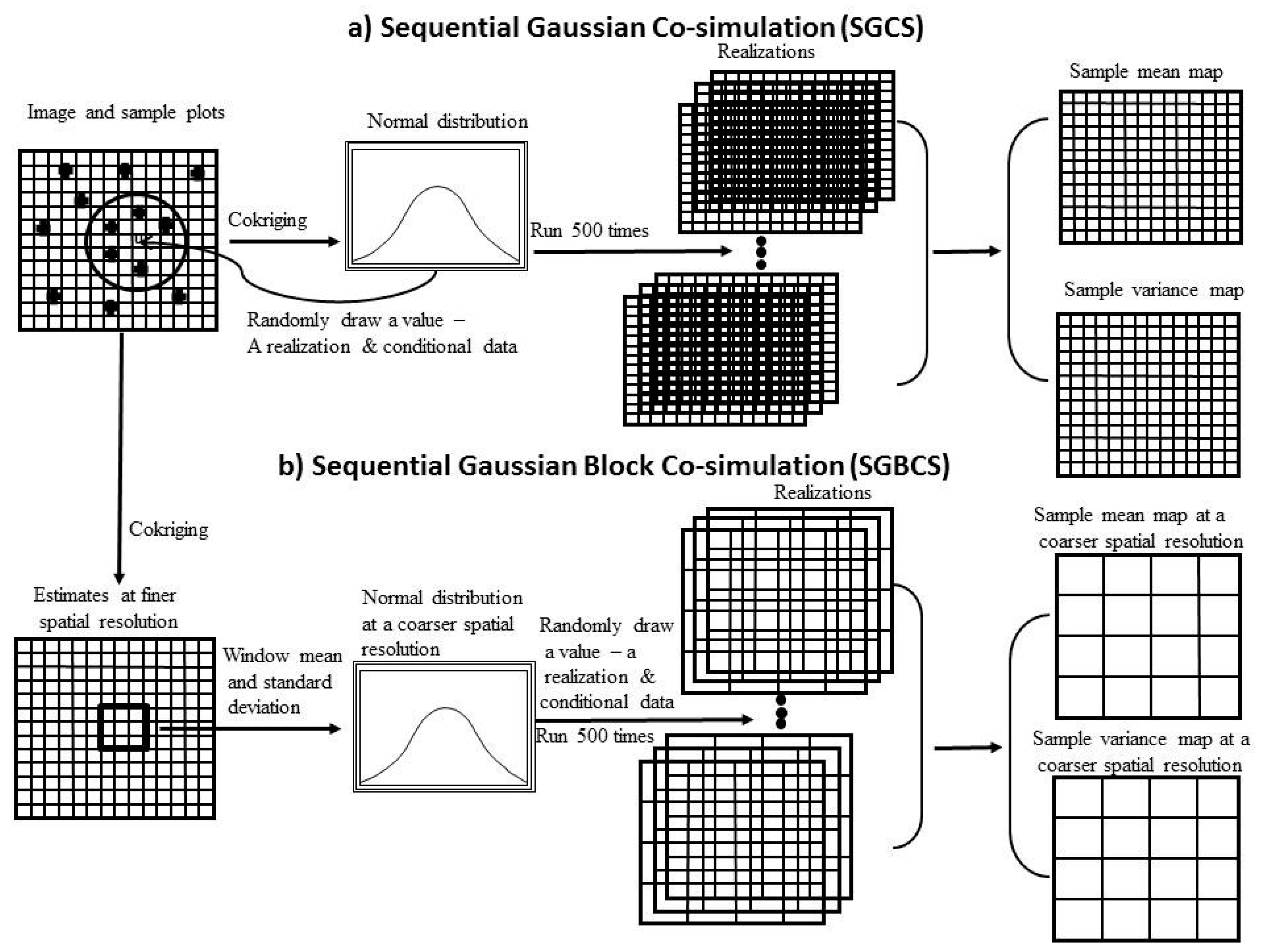[34] employed fine spatial resolution Geoeye-1 and QuickBird-2 images and harmonizing Fourier textural ordination to detect forest canopy structural heterogeneity in Central Africa and further developed piecewise biomass inversion models using 26 inventory plots (1 ha) to predict AGB variations. However, these methods lack the capacity of modeling propagation of input uncertainties from a finer spatial resolution to a coarser one and of generating spatial distributions of up-scaled estimates and their uncertainties. For this purpose, Wang et al. [27] developed a spatial variability-based sequential Gaussian block co-simulation (SGBCS) algorithm in which both spatial data and their uncertainties can be scaled up from a finer spatial resolution to any coarser ones, leading to maps of estimates and their uncertainties at coarser spatial resolutions. This method has been applied to mapping and spatial uncertainty analysis of forest carbon density [20,31].

On the other hand, the accuracy of forest carbon density maps is often assessed using root mean square error (RMSE) between estimated and observed values [35,36]. There have been three methods for obtaining these field observations. First, a set of sample plots is often randomly divided into two sub-sets. One sub-set of data is applied for model development and another for validation of obtained models. This method is limited due to the sample plots used for accuracy assessment are not independent from those used for model development. Secondly, cross-validation can be used for accuracy assessment [37,38]. This method greatly saves time and money for collection of field plot data, but means an intensive computation. The best way for accuracy assessment is the acquisition and application of independent sample plots, but this is time- and money-consuming. Additionally, a spatial uncertainty and error budget method can be used [20,27,31,39,40,41]. In this method, various sources of errors are identified, quantified and linked with the output uncertainties, and the contributions of various input errors to the output uncertainties are then calculated. However, this method is relatively complicated. Generally, the accuracy assessment of forest carbon density estimates requires consistent spatial resolutions between the derived forest carbon density maps and sample plot data. When the spatial resolutions are inconsistent, or multiple spatial resolution maps of forest carbon density have to be derived, the accuracy assessment will become a great challenge [27]. Thus far there have been some studies reported in this area [11,20,27,31,32,33,34,35]. However, further study is still needed toward the development of an effective sampling design and an algorithm that can be used to map forest carbon density and conduct accuracy assessment at multiple spatial resolutions.

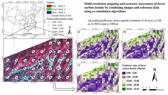
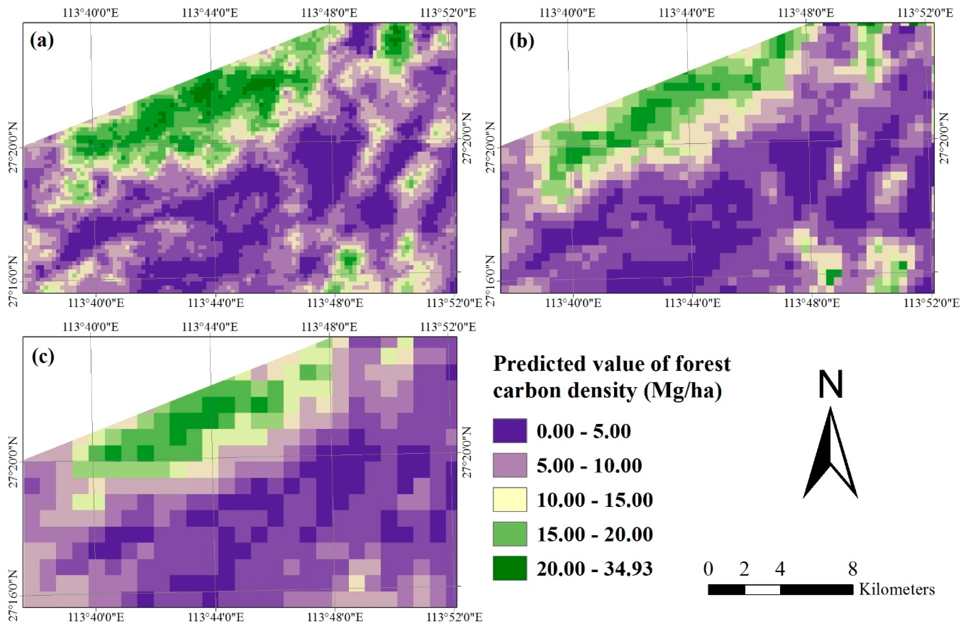
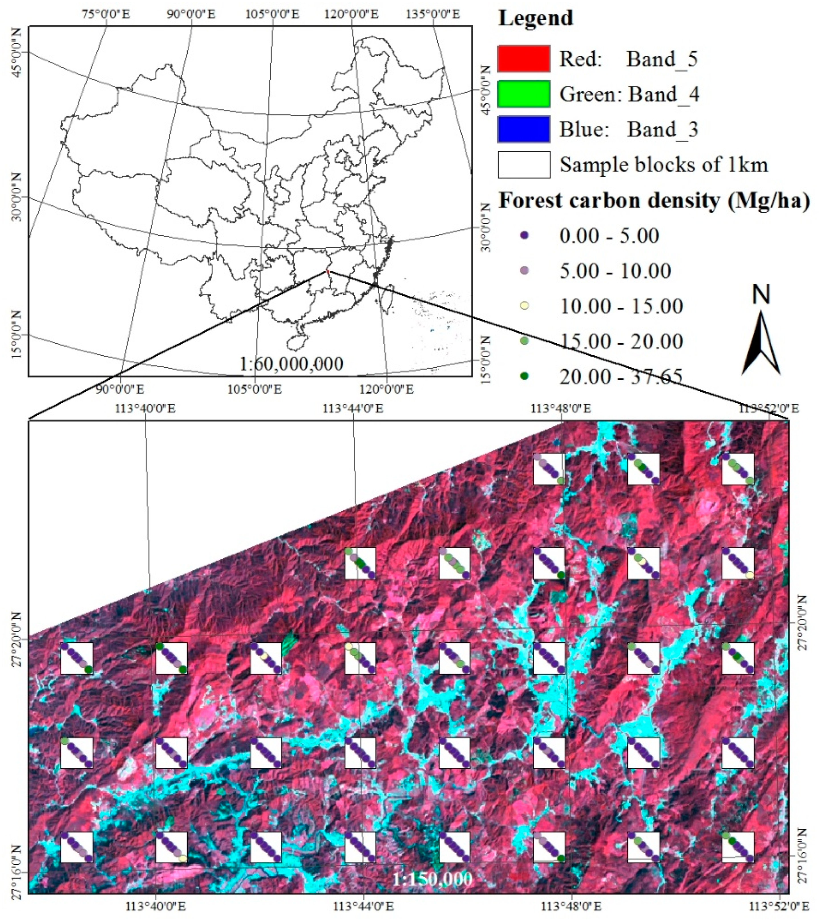
The purpose of this study was to develop a methodological framework for mapping and accuracy assessment of forest carbon density at four spatial resolutions by combining images from Landsat 8 and MODIS and four reference datasets from a systematical, nested and clustering sampling design. This study was carried out in Huang-Feng-Qiao forest farm of You County in Hunan of China. The used images had four spatial resolutions of 30 m × 30 m, 250 m × 250 m, 500 m × 500 m and 1000 m × 1000 m. An image-based sequential Gaussian co-simulation algorithm (SGCS) and SGBCS approach developed by Wang et al. [20,27,31] were employed to map forest carbon density at the spatial resolutions. Moreover, this study compared the accuracies of up-scaled estimates derived by scaling up a SGCS and Landsat derived 30 m resolution map with a window average (WA) (called SGCSWA algorithm), combining Landsat 8 and SGBCS, and combining MODIS images and SGCS, and demonstrated the potential of the methodology to provide the spatial information of forest carbon density at multiple spatial resolutions.

2. Materials and Methods

2.1. Study Area

Huang-Feng-Qiao forest farm of You County is located in Eastern Hunan of China with latitude and longtitude ranges of 27°06’N to 27°24’N and 113°04’E to 113°43’E, respectively (Figure 1). This area is in a typical subtropical climate region with the average annual temperature of 17.8° and the annual precipitation of 1411 mm [42]. Its elevation varies from 0 to 1132 m above sea level. It is dominated by mountainous areas with a slope range of 0 to 57 degrees. The landscape is complex and fragmented. The dominant forests include coniferous planations; evergreen broad-leaved forests; coniferous, deciduous and evergreen broad-leaved mixed forests with scattered bamboo stands; shrubs; and agricultural lands. The dominant tree species are Cunninghamia lanceolata (Lamb.)Hook, Pinus massoniana Lamb, Pinus elliottii, Cinnamomum camphora (L.) Presl, Liriodendron chinense (Hemsl.) Sarg, Cupressus funebris Endl, and Alnus cremastogyne Burk and Phoebe zhennan S. Lee. This area has a forested land of 10,123, representing 86% forest cover.

2.2. Datasets

2.2.1. Sample Plot Data

In this study area, a total of 32 sample blocks were systematically allocated from 15 July to 10 August 2013 with a sampling distance of 3 km. Each blocks had a size of 1000 m × 1000 m (100 ha). Within each block, there were 7 sample plots with a size of 30 m × 30 m designed along its diagonal line from northwest to southeast (Figure 1). That is, there were a total of 224 sample plots selected within the study area. When a sample plot fell into a forested land, dipping angle gauge control was adopted to collect field observations of forest stand variables including dominant tree species, crown density, tree diameter at breast height, basal area at breast height, crown width, and tree height. If a sample plot fell into a non-forested land, only the vegetation type was recorded. The sampling was described in detail in the section of a systematical, nested and clustering sampling.

The sample plots were located with differential global positioning system (GPS) units. Within each sample plot, tree height and diameter at breast height were measured and used to estimate tree AGB (trunk, branch, bark and leaf) by tree species using empirical models (

Table 1. Biomass regression models and biomass-to-carbon conversion coefficients by tree species and groups (W_S: Stem biomass; W_P: Bark biomass; W_B: Branch biomass; W_L: Leaf biomass; W_T: Total aboveground biomass; D: tree diameter at breast height; H: tree height).

Tree Species and Group	Biomass Regression Models	Biomass-to-carbon Conversion Coefficiets
Chinese fir and similar species group	${\widehat{W}}_S=0.073429(D^{2}H{)}^{0.86262};{\widehat{W}}_P=0.013775(D^{2}H{)}^{0.84463};$ ${\widehat{W}}_B=0.000482(D^{2}H{)}^{1.23314};{\widehat{W}}_L=0.019638(D^{2}H{)}^{0.78969};$ ${\widehat{W}}_T={\widehat{W}}_S+{\widehat{W}}_P+{\widehat{W}}_B+{\widehat{W}}_L$	0.52
Pinus massoniana and similar species group	${\widehat{W}}_T=0.071556(D^{2}H{)}^{0.857209}$	0.46
Hardwood broad-leaved tree species group	${\widehat{W}}_S=0.044(D^{2}H{)}^{0.9169};{\widehat{W}}_P=0.023(D^{2}H{)}^{0.7115};$ ${\widehat{W}}_S=0.044(D^{2}H{)}^{0.9169};{\widehat{W}}_P=0.023(D^{2}H{)}^{0.7115};$ ${\widehat{W}}_T={\widehat{W}}_S+{\widehat{W}}_P+{\widehat{W}}_B+{\widehat{W}}_L$	0.48
Softwood broad-leaved tree species group	${\widehat{W}}_T=0.0495502(D^{2}H{)}^{0.952453}$	0.50
Eucalyptus	${\widehat{W}}_S=0.0902526D^{2.44815};{\widehat{W}}_B=0.0049163D^{2.81779};$ ${\widehat{W}}_L=0.012694D^{2.26839};{\widehat{W}}_T={\widehat{W}}_S+{\widehat{W}}_B+{\widehat{W}}_L$	0.53
Bamboo	${\widehat{W}}_T=0.6439D^{1.5373}$	0.50

) proposed by Li et al. [43]. The values of tree AGB were converted to the values of forest carbon density using biomass-to-carbon coefficients by tree species and then summed to obtain the plot value. Because some of the species did not have any biomass models and carbon conversion coefficients, similar tree species models and coefficients were employed to approximate their values of forest carbon density. There were also no empirical models and carbon conversion coefficients available for the shrubs, and average biomass values of 23.7 Mg/ha and 19.76 Mg/ha were used, respectively [44]. The obtained AGB was then converted to forest carbon using a coefficient of 0.5. Using the allometric models, especially those for similar species, and the average biomass values for the shrubs would definitely lead to uncertainty of biomass and carbon estimates. However, in this study, this uncertainty was considered to be negligible.

2.2.2. Remotely Sensed Data

In this study, a Landsat 8 image dated 17 September 2013 and with a cloud cover of less than 10% was acquired with a spatial resolution of 30 m × 30 m same as that of the sample plots. This image consisted of seven bands: band 1—Coastal, band 2—Blue, band 3—Green, band 4—Red, band 5—near infrared (NIR), band 6—short wavelength infrared 1 (SWIR1) and band 7—short wavelength infrared 2 (SWIR2). The digital values of image pixels were first converted into the values of spectral reflectance using ENVI radiometric calibration and FLAASH atmospheric correction tool. In order to reduce the effects of shade, topographic correction was then conducted for the image using Minneart model. Finally, geometric correction was made using a topographic map with RMSE less than one pixel. Moreover, three MODIS products including MOD13Q1, MOD09A1 and MOD15A2 dated on 14 September 2013 were collected for mapping forest carbon density at the spatial resolutions of 250 m × 250 m, 500 m × 500 m and 1000 m × 1000 m, respectively. For the MODIS images, the data pre-processing including projection transformation, image mosaic and image mask were conducted using ENVI. In addition, cloud in the images was removed using a program written by the IDL language [45]. In this study, Landsat and MODIS images were selected partly because they are most widely utilized to map forest carbon density at various scales and partly because the cost to collect LiDAR and RADAR data is not affordable, especially for very large areas. In addition, this study aimed at developing a general methodology in which widely used remotely sensed images for mapping forest carbon density should be selected.

2.2.3. Image Transformations

For Landsat 8 image, first, in addition to the original seven bands, their inversions were calculated, leading to seven new bands. Second, various band ratios such as $S{R}_{i,j}=Ban{d}_i/Ban{d}_j$, $S{R}_{i,j,k}=Ban{d}_i/(Ban{d}_j+Ban{d}_k)$, $i,j,k=1,\mathrm{...},7,$ $i\ne j\ne k$, $j<k$ and so on, were also calculated, resulting in a total of 147 spectral variables. Third, five vegetation indices were generated, including normalized differential vegetation index (NDVI), soil adjusted vegetation index (SAVI) with two different coefficients, atmospherically resistant vegetation index (ARVI) and enhanced vegetation index (EVI). Moreover, principal component analysis of the original seven bands from Landsat 8 image was carried out and the first three components that accounted for 99% of total variance were selected. Additionally, a total of 56 texture variables from gray-level co-occurrence-matrix-based texture measures (mean, angular second moment, contrast, correlation, dissimilarity, entropy, homogeneity, and variance) were calculated. Finally, a total of 225 spectral variables were obtained. The objectives for calculating band ratios, vegetation indices and texture measures were to reduce the effects of slope in the mountainous areas and quantify the canopy structures and their spatial variability of the complicated and fragmented landscape.

For MODIS 500 m × 500 m products, the above five groups of the image transformations used for Landsat 8 image were calculated and the used bands included band 1, band 2, band 3, band 4, band 6 and band 7. A total of 158 spectral variables were obtained. For MODIS 250 m × 250 m and 1000 m × 1000 m products, in addition to vegetation indices NDVI and EVI, four reflectance bands (band 1—Red, band 2—NIR, band 3—Blue and band 4—medium infrared (MIR)) were used to calculate the above five groups of image transformations, leading to a total of 87 spectral variables for each of the spatial resolutions.

2.3. Systematical, Nested and Clustering Sampling Design

To collect reference values of forest carbon density at multiple spatial resolutions, 32 of 1000 m × 1000 m blocks were systematically designed with a 3 km sampling distance to cover the study area (Figure 1). Within each of the 1000 m × 1000 m blocks, a 30 m × 30 m sample plot was located at the block center and two sub-blocks with sizes of 250 m × 250 m and 500 m × 500 m and the same centers were nested (Figure 2). Another six 30 m × 30 m sample plots within the sub-blocks and blocks were systematically allocated along the diagonal lines from northwest to southeast. The sample plots were spatially allocated as follows: (1) Within each 250 m × 250 m sub-block, in addition to the block centered 30 m × 30 m sample plot, two other sample plots were added at the middle points of the diagonal line from the center to the northwest and southeast corners, respectively. Thus, a total of three sample plots were used to capture the characteristics of forests in each 250 m × 250 m sub-block; (2) Because each 250 m × 250 m sub-block was nested in each 500 m × 500 m sub-block, the previous three sample plots could be used. Additionally, two other sample plots were, respectively, added at the middle points from the northwest and southeast corners of the 250 m × 250 m sub-block to the northwest and southeast corners of the 500 m × 500 m sub-block. A total of five sample plots were thus obatined to provide the information of forests for each 500 m × 500 m sub-block; (3) In a similar way, two more sample plots were added for each 1000 m × 1000 m block, which led to a total of seven sample plots to capture the spatial variability of forests within the block (Figure 2). This design resulted in four reference datasets with four spatial resolutions matching the pixel sizes of the used images, 30 m × 30 m, 250 m × 250 m, 500 m × 500 m and 1000 m × 1000 m, and aimed to provide the potential of obtaining reference values of forest carbon density at four spatial resolutions.

A total of 224 sample plots that matched the spatial resolution of 30 m × 30 m were obtained over the study area. For each of the 250 m × 250 m sub-blocks, three forest carbon density values from three sample plots were averaged and used to represent the average forest carbon density for 250 m spatial resolution MODIS image. Similarly, the average values of forest carbon density were calculated from five and seven sample plots for 500 m and 1000 m spatial resolution MODIS images respectively. The central coordinates of the blocks and sub-blocks were used to extract the pixel values of the images. This design was similar to a systematical, nested and clustering sampling. A systematical sampling distance for these clusters (that is, the 250 m and 500 m sub-blocks and 1000 m blocks) was utilized and the sampling distances between the sample plots within each cluster were unequal, but fixed. Standard deviation and coefficient of variation at the sub-block and block levels were thus calculated considering the features of clustering sampling [46]. Because only the trees within three, five and seven 30 m × 30 m sample plots were measured for the 250 m and 500 m sub-blocks and 1000 m block, the average values calculated from the sample plots were used to represent the sub-blocks and blocks. The average values were thus associated with uncertainty and called reference values.

2.4. Spatial Co-Simulation Algorithms to Generate Forest Carbon Density Maps

In this study, an image-based SGCS algorithm developed by Wang et al. [20,27,47,48] was utilized to generate forest carbon density maps at the spatial resolutions of Landsat 30 m × 30 m and MODIS 250 m × 250 m, 500 m × 500 m and 1000 m × 1000 m. In this algorithm, it is assumed that a study area consists of N pixels that have the same spatial resolution with the reference data from the sample plots (Figure 3a). It is also assumed that forest carbon density is a random process that consists of random variables z(u) that are spatially auto-correlated with each other. The spatially auto-correlated variables mean forest carbon density at the image pixels. The value of forest carbon density at each pixel has to be generated and can be regarded as a realization of the random variable at this location.

To obtain a realization at each pixel, first a spatial auto-correlation model of forest carbon density must be developed by calculating an experimental variogram—spatial variability function over the distance between data locations given a direction and then fitting the variogram using theoretical variance functions such as spherical, Gaussian and exponential model [20,27,47,48]. The obtained variogram accounts for the spatial variability of forest carbon density. Generally, as the distance between data locations increases, the spatial variability increases until reaching its maximum value. The distance that corresponds to the maximum variance is called the range parameter of the model implying the maximum distance of spatial auto-correlation.

Second, in the algorithm, a random path for visiting and estimating each of the pixels for the study area is determined using a generator of random numbers. Following this path, each pixel is visited and a conditional cumulative distribution function (CCDF) (mean and variance) of forest carbon density at this pixel is derived using an unbiased cokriging estimator by weighting the forest carbon density reference values, image pixel values and existing estimates if any within a neighborhood determined by the maximum spatial auto-correlation distance (Figure 3a). The weights vary depending on the variogram and the distance of the pixel to be estimated to the data locations. Generally, the shorter the distance is, the greater the weight becomes. From CCDF, a value can be randomly drawn and used as a realization of forest carbon density at this pixel. The realization can be utilized as a conditional datum for next simulation. When all of the pixels are visited and yield their realizations of forest carbon density, a map of forest carbon density is obtained.

Generating and using a large number of random paths and repeating the above co-simulation process can lead to many realizations for each pixel. In this study, after an experiment it was found that a total of 500 random paths resulted in a stable variance of the realizations. Across the realizations, a sample mean and variance of forest carbon density were calculated for each pixel and used as its predicted value and uncertainty measure respectively (Figure 3a). This algorithm is based on the assumption that forest carbon density has a Gaussian distribution and if not, normal score transformation of data should be conducted for both the reference values and image data. The aforementioned algorithm was used to generate the maps of forest carbon density at the spatial resolution of 30 m × 30 m with the spectral variables derived from Landsat 8 image, and at the spatial resolutions of 250 m × 250 m, 500 m × 500 m and 1000 m × 1000 m with the spectral variables from MODIS products.

In addition, an image-based up-scaling algorithm SGBCS (Figure 3b) was utilized to generate the maps of forest carbon density at the spatial resolutions of 250 m × 250 m, 500 m × 500 m and 1000 m × 1000 m by combining and scaling up the forest carbon density plot data and the Landsat image at the original spatial resolution of 30 m × 30 m [20,27,48]. The block co-simulation is similar to the above SGCS. The difference is that in this algorithm each sub-block or block is considered to consist of many smaller 30 m × 30 m pixels. Each of the smaller pixels is first estimated using an unbiased cokriging estimator (Figure 3b). The CCDF of the sub-block or block is then derived by calculating a window mean and variance of the predicted values of the smaller pixels, and used for spatial co-simulation at sub-block and block levels.

It had to be pointed out that when the SGCS and SGBCS algorithms were used to create the forest carbon density maps at the multiple spatial resolutions, the features of a systematical, nested and clustering sampling with an equal sampling distance between the sub-blocks and blocks and unequal, but fixed sampling distances between the sample plots within each of the sub-blocks and blocks were taken into account by using a de-clustering method to derive the weights of the sample plots. In order to find appropriate spectral variables from the image bands and their transformations, the spectral values of the sample plots, sub-blocks and blocks were extracted using ArcMap. Pearson product moment correlation coefficients between the spectral variables and forest carbon density were calculated and ranked. The spectral variable that had the highest correlation was used to create a map of forest carbon density at each of the spatial resolutions.

2.5. Accuracy Assessment and Algorithm Comparison

The correlation coefficients between the spectral variables and forest carbon density were statistically tested for their significant differences from zero using the equation $r_{\alpha }=\sqrt{t_{\alpha }^2/\left(n-2+t_{\alpha }^2\right)}$ based on the student’s distribution at a significance level of α = 0.05, where n is number of sample plots used. Moreover, when Landsat image was used to create the forest carbon density map at the spatial resolution of 30 m × 30 m, 50 sample plots were randomly selected from the total of 224 sample plots and used for accuracy assessment of predicted values and the rest 174 sample plots were used to conduct the spatial co-simulation. For generation of forest carbon density maps at the coarser spatial resolutions of 250 m × 250 m, 500 m × 500 m and 1000 m × 1000 m, a method called k-fold cross-validation was applied to carry out the accuracy assessment. In this method, each dataset was divided into k sub-sets, each time one sub-set of the reference data was took out from the dataset and utilized as a validation dataset. The remaining sub-sets of the data were employed as the training dataset for the co-simulation of forest carbon density. Repeating this process k times led to k sub-sets of estimation errors. A RMSE and relative RMSE were thus calculated and the features of clustering sampling were considered at the sub-block and block levels. In this study, four fold cross-validations were used for the accuracy assessment of the forest carbon density maps at the coarser spatial resolutions. The accuracy of forest carbon density was also quantified using the overall bias (that is, residual mean), coefficient of determination R² and slope value of the relationship between the reference and predicted values for each spatial resolution [49].

In addition, this study led to the maps that can be used as stand-alone products that depict the spatial distribution of forest carbon density for this study area. The evaluation with respect to the applications of the maps was made by calculating the map means of predicted forest carbon density values using a model-assisted regression estimator. Based on the reference datasets from the sampling design and four spatial resolution images from Landsat and MODIS, the following forest carbon density maps were generated and compared:

(1)

A forest carbon density map at the spatial resolution of 30 m × 30 m was created by combining the Landsat 8 image and the dataset of 174 sample plots used for modeling using SGCS and the accuracy of this map was assessed using the validation dataset of 50 sample plots.

(2)

The predicted values of the above 30 m spatial resolution map from SGCS were scaled up to the spatial resolutions of 250 m × 250 m, 500 m × 500 m and 1000 m × 1000 m using a window average method (WA) [27]. This method was an integration of SGCS and WA and denoted as SGCSWA. The accuracies of the coarser spatial resolution maps were assessed by comparing the predicted and reference values at the sampled locations for the spatial resolutions.

(3)

The forest carbon density maps at the spatial resolutions of 250 m × 250 m, 500 m × 500 m and 1000 m × 1000 m were also generated by combining and scaling up the 30 m spatial resolution Landsat 8 image and the sample plot dataset using SGBCS. Four fold cross-validations were used for the accuracy assessment of the maps.

(4)

The forest carbon density maps at the spatial resolutions of 250 m × 250 m, 500 m × 500 m and 1000 m × 1000 m were produced by combining the MODIS images and the reference datasets using SGCS. Four fold cross-validations were used for the accuracy assessment of the maps.

3. Results

3.1. Statistical Analysis of Sample Plot Data

Table 2. Statistics of forest carbon density for the sample plots at four spatial resolutions (Note: SD = standard deviation; CV = coefficient of variation).

Spatial Resolutions (SR) and Datasets	Sample Statistical Parameters
	N. of Plots, Sub-blocks & Blocks	Minimum (Mg/ha)	Maximum (Mg/ha)	Mean (Mg/ha)	SD (Mg/ha)	CV (%)
30 m × 30 m SR plot dataset	224	0.00	37.65	8.81	9.35	106.16
30 m × 30 m SR plot dataset for modeling	174	0.00	37.65	8.41	9.11	108.21
30 m × 30 m SR plot dataset for validation	50	0.00	34.14	10.18	10.13	99.55
250 m × 250 m sub-block dataset	32	0.00	25.14	9.85	1.25	12.67
500 m × 500 m sub-block dataset	32	0.00	23.57	9.32	1.15	12.36
1000 m × 1000 m block dataset	32	0.00	22.16	8.81	1.03	11.68

presented the statistics of forest carbon density from the sample plots at four spatial resolutions: 30 m × 30 m, 250 m × 250 m, 500 m × 500 m and 1000 m × 1000 m. As the spatial resolution became coarser, the values of maximum, standard deviation and the coefficient of variation (CV) for the reference data from the sample plots, sub-blocks and blocks decreased. The dataset from all of the 224 sample plots had a sample mean of 8.81 Mg/ha with a CV of 106.16%. This CV value was relatively large. When the dataset was randomly divided into two for modeling and validation respectively, the validation dataset got a slightly greater sample mean with a slightly smaller CV. The sample mean of the reference dataset for 1000 m × 1000 m blocks was the same as that from all of the sample plots because all of the plots fell in the blocks. The sample means of the reference datasets for 250 m × 250 m and 500 m × 500 m sub-blocks were slightly greater than that from all of the sample plots because of the four and two sample plots, respectively, ignored for each kind of sub-block. The standard deviation and CV values at the sub-block and block levels were much smaller than those at the plot level because the sample plot data within the sub-blocks and blocks were averaged with the features of clustering sampling taken into account (Table 2).

3.2. Correlation Analysis between Spectral Variables and Forest Carbon Density

The correlation coefficients of the spectral variables with forest carbon density reference data from the sample plots, sub-blocks and blocks, varied from −0.395 to 0.499 and −0.664 to 0.738 for Landsat 8 and MOD09A1 images, respectively. Based on the significant value at the significant level of 0.05, among the 225 and 158 spectral variables a total of 28 and 22 spectral variables were statistically significantly correlated with forest carbon density for Landsat 8 and MOD09A1 images, respectively. For MOD13Q1 and MOD15A2 images, the respective correlation coefficients ranged from −0.638 to 0.663 and −0.491 to 0.455. At the significance level of 0.05, out of 78 spectral variables there were, respectively, 19 and 10 spectral variables that had significant correlation with forest carbon density. The texture measures from MODIS images significantly improved the correlation with forest carbon density, implying they quantified the information of canopy structures and forest heterogeneity more accurately than other spectral variable. Because of limited space, most of the correlation results were omitted and only the six most correlated variables were listed in

Table 3. Pearson product moment correlation coefficients of forest carbon density with spectral variables.

Images–Spatial Resolution
Landsat 8-30 m		MOD13Q1-250 m		MOD09A1-500 m		MOD13A2-1000 m
Variable	Correlation	Variable	Correlation	Variable	Correlation	Variable	Correlation
Band1/R	0.499 *	NDVIsec	0.663 *	1/R	0.738 *	NIRsec	0.491 *
Band1/(B+SWIR2)	0.492 *	NDVIent	0.638 *	1/G	0.707 *	MIRmean	0.489 *
Band1/(R+SWIR2)	0.490 *	NDVIhom	0.617 *	R/SWIR1	0.664 *	Rmean	0.487 *
1/SWIR1	0.483 *	1/B	0.602 *	1/B	0.663 *	Blmean	0.463 *
1/SWIR2	0.477 *	Bmean	0.600 *	Gmean	0.649 *	EVIcor	0.455 *
Band1/(G+R)	0.460 *	1/R	0.572 *	G/SWIR1	0.646 *	NDVIent	0.450 *

Note: * indicating a significant correlation at a significance level of α = 0.05; B, G, R, NIR, SWIR1, SWIR2, MIR, NDVI, and EVI are the bands of blue, green, red, near infrared, short wavelength infrared 1, short wavelength infrared 2, middle infrared, normalized difference vegetation index and enhanced vegetation index; and the subscripts mean, sec, cor, ent, and hom, represent the texture measures from mean, second moment, correlation, entropy, and homogeneity, respectively.

. A spectral variable that was most correlated with forest carbon density was found for each of the spatial resolution images. The most correlated spectral variables band1/Red for Landsat 8, NDVI_sec for MOD13Q1, 1/Red for MOD09A1, and NIR_sec for MOD13A2 were used to conduct the spatial co-simulations and mapping forest carbon density with the corresponding spatial resolution images, where subscript “sec” means second moment. Two of the selected spectral variables were related to red band because trees use the energy in these wavelengths for photosynthesis and creating biomass. Moreover, the band ratio (band 1/Red) helped reduce the effect of slope in this mountainous area. All other selected spectral variables were derived from a gray-level co-occurrence-matrix-based texture measure, angular second moment, and captured the canopy structures and spatial variability of the complicated and fragmented landscape.

3.3. Spatial Variability Analysis of Forest Carbon Density

The standardized experimental variogram of forest carbon density was calculated using the reference values from the sample plots and then fit using variance functions spherical, exponential and Gaussian models. The selection of the models was conducted based on the coefficient of determination R² between the estimated and observed values, goodness of fit and residual sum of squares (RSS) (

Table 4. Parameters of standardized variogram models for forest carbon density (R² is the coefficient of determination and RSS means the residual sum of squares).

Model	R2	RSS	Goodness of Fit	Nugget Parameter	Structural Parameter	Range (km)
Spherical	0.78	0.0575	1.3725 × 10−3	0.73	0.27	15.62
Exponetial	0.68	0.0628	2.0993 × 10−3	0.69	0.31	14.91
Gaussian	0.72	0.0623	1.7818 × 10−3	0.71	0.29	12.98

). The greater the R² and the smaller the goodness of fit and RSS, the more accurate the fitting was. The results showed that the spherical model Equation (1) led to the greatest R² value and the smallest values for goodness of fit and RSS. The aforementioned co-simulation algorithms require that the parameters of the variogram models be standardized, that is, the nugget plus structure parameter (variance change rate) equals to one unit because the normal score transformation of spatial data was conducted. The nugget value means the within sample plot variation and measurement error of forest carbon density, the structural parameter implies the change rate of variance over the distance between data locations, and the range parameter is the maximum distance of spatial auto-correlation. Within the range, data values are spatially auto-correlated with each other and out of the range they tend to be independent to each other. In Equation (1), h with unit km is the distance between data locations. The spherical model selected led to a relatively larger nugget parameter and smaller structure parameter, which indicated that the spatial auto-correlation existed, but was not very strong. This may be attributed to the complicated and fragmented forest landscape.

Spherical model:

$$\gamma (h)=0.73+0.27\times [1.5\times \frac{h}{15.62}-0.5\times {(\frac{h}{15.62})}^3]$$

(1)

3.4. Up-Scaling of Forest Carbon Density Using SGCSWA and SGBCS Based on Landsat 8 Image

Table 5. Accuracy assessment results of predicted forest carbon density values by combining Landsat 8 image and sample plot data at the spatial resolution of 30 m × 30 m using sequential Gaussian co-simulation (SGCS), and at the spatial resolutions of 250 m × 250 m, 500 m × 500 m and 1000 m × 1000 m by SGCSWA (R² and RMSE are the coefficient of determination and root mean square error between the predicted and reference values; the confidence intervals at the significance level of 0.05 are (7.37, 12.94), (7.73, 11.96), (7.37, 11.27) and (6.07, 10.56) (Mg/ha) for the 30 m, 250 m, 500 m and 1000 m spatial resolutions respectively).

Image-Resolution and Method	Predicted Mean (Mg/ha)	Residual Mean (Mg/ha)	Relationship between Reference and Predicted Values	R2	RMSE (Mg/ha)	Relative RMSE
Landsat 8-30 m by SGCS	10.51	−0.33	y = 1.02x − 0.53	0.88	3.44	33.76
Landsat 8-250 m by SGCSWA	9.93	−0.08	y = 1.28x − 2.86	0.85	0.54	5.45
Landsat 8-500 m by SGCSWA	9.25	0.07	y = 1.08x − 0.69	0.80	0.51	5.51
Landsat 8-1000 m by SGCSWA	8.84	−0.03	y = 1.06x − 0.56	0.79	0.49	5.52

presents the accuracies of predicted forest carbon density values at the spatial resolution of 30 m × 30 m by SGCS, and at the spatial resolutions of 250 m × 250 m, 500 m × 500 m, and 1000 m × 1000 m by SGCSWA. Overall, the means of predicted values were close to those of reference datasets and fell in the confidence intervals of the reference data at the significant level of 0.05. The mean was slightly over-predicted at the spatial resolution of 30 m × 30 m by SGCS. When the predicted values of the 30 m spatial resolution map was scaled up to the coarser spatial resolutions by SGCSWA, the amounts of the over- and under-predictions for the mean could be ignored (Table 5). Moreover, the coefficients of determination between the reference and predicted values were significantly different from zero and over 79% of the variability of the reference values was explained by the predicted values. The slope values of the linear relationships between the reference and predicted values were slightly larger than, but not significantly different from one for all of the spatial resolutions except the pixel size of 250 m, and all of the intercepts were negative. The slope and intercept values implied that over-predictions and under-predictions occurred for the smaller and larger reference values respectively. The RMSE and relative RMSE were large at the 30 m spatial resolution plot level and both greatly decreased after the spatial data were scaled up to the coarser spatial resolutions. At the sub-block and block levels, as the pixel size increased from 250 m × 250 m to 500 m × 500 m and 1000 m × 1000 m, overall the RMSE values slightly decreased and the relative RMSE values slightly increased (Table 5). In Figure 4, the residuals of the predicted values were graphed against the predictions at all of the spatial resolutions and they were scattered at both sides of zero line and did not show any biased trends.

Table 6. Accuracy assessment results of predicted forest carbon density values at the spatial resolutions of 250 m × 250 m, 500 m × 500 m and 1000 m × 1000 m by combining and scaling up Landsat 8 image and sample plot data using sequential Gaussian block co-simulation (SGBCS) (R² and RMSE are the coefficient of determination and root mean square error between the predicted and reference values; The confidence intervals at the significance level of 0.05 are (7.73, 11.96), (7.37, 11.27) and (6.07, 10.56) (Mg/ha) for the 250 m, 500 m and 1000 m spatial resolutions, respectively).

Image-Resolution and Method	Predicted Mean (Mg/ha)	Residual Mean (Mg/ha)	Relationship between Reference and Predicted Values	R2	RMSE (Mg/ha)	Relative RMSE
Landsat8-250 m	10.12	−0.27	y = 1.19x − 2.14	0.81	0.57	5.77
Landsat8-500 m	9.46	−0.14	y = 1.12x − 1.28	0.79	0.54	5.83
Landsat8-1000 m	8.06	0.75	y = 1.17x − 0.65	0.77	0.52	5.93

shows the accuracies of predicted forest carbon density values at the spatial resolutions of 250 m × 250 m, 500 m × 500 m, and 1000 m × 1000 m using SGBCS based on Landsat 8 image. Although, overall, the means were slightly over-predicted at the spatial resolutions of 250 m × 250 m and 500 m × 500 m and under-predicted at the spatial resolution of 1000 m × 1000 m, they fell in their confidence intervals of reference data at the significant level of 0.05 (Table 6). Moreover, the coefficients of determination between the reference and predicted values were significantly larger than zero and the predicted values accounted for over 77% of the variability of the reference values. However, the slope values of the linear relationships between the reference and predicted values were larger than one with all of the negative intercepts for all of the spatial resolutions. The slope and intercept values indicated over-predictions and under-predictions taking place for the smaller and larger reference values, respectively. There were no significant differences of RMSE and relative RMSE among three spatial resolutions, but the RMSE values slightly decreased and the relative RMSE slightly increased as the spatial resolutions became coarser (Table 6). In the graph for the residuals of the predicted values against the predictions at the three spatial resolutions, the residuals were scattered at both sides of zero line (this figure was given in Supplementary Materials Figure S1).

The forest carbon density and its variance maps obtained using SGCS at the spatial resolution of 30 m × 30 m are shown in Figure 5. The maps had similar spatial distributions and also similar to that of the forests from the sample plot data and shown in Landsat color infrared composite image at the spatial resolution of 30 m × 30 m. The larger prediction values of forest carbon density existed in the north, northwest central, northeast, and scattered in the southeast. In the areas where the predicted values were greater, the corresponding variances of the predicted values were also greater. When the 30 m spatial resolution map was scaled up to the coarser spatial resolutions by SGCSWA, the spatial patterns of the predicted values were similar to that at the 30 m spatial resolution (omitted because of limited space). However, the predicted values were greatly smoothed and the smoothing became more obvious as the pixel sizes became larger. The maps of forest carbon density derived at the spatial resolutions of 250 m × 250 m, 500 m × 500 m, and 1000 m × 1000 m using SGBCS are presented in Figure 6. They had similar spatial patterns of forest carbon density. However, the smoothing of the predicted values was obviously noticed.

3.5. Generation of Forest Carbon Density Maps Using Coarse Spatial Resolutions MODIS Products

The cross-validation accuracies of predicted forest carbon density values by combining MOD13Q1, MOD09A1 and MOD13A2 products and the reference values from the sample plots within the sub-blocks or blocks using SGCS at the spatial resolutions of 250 m × 250 m, 500 m × 500 m and 1000 m × 1000 m are shown in

Table 7. Cross-validation accuracy assessment results of predicted forest carbon density values at the spatial resolutions of 250 m × 250 m, 500 m × 500 m and 1000 m × 1000 m by combining MODIS products and the reference values of the sample plots within the sub-blocks and blocks using sequential Gaussian co-simulation (SGCS) (R² and RMSE are the coefficient of determination and root mean square error between the predicted and reference values; the confidence intervals at the significance level of 0.05 are (7.73, 11.96), (7.37, 11.27) and (6.07, 10.56) (Mg/ha) for the 250 m, 500 m and 1000 m spatial resolutions, respectively).

Image-resolution and Method	Predicted Mean (Mg/ha)	Residual Mean (Mg/ha)	Relationship between Reference and Predicted Values	R2	RMSE (Mg/ha)	Relative RMSE
MOD13Q1-250 m	8.96	0.88	y = 0.99x + 0.94	0.76	0.63	6.38
MOD09A1-500 m	8.24	1.08	y = 1.02x + 0.88	0.73	0.62	6.70
MOD13A2-1000 m	7.58	1.23	y = 1.10x + 0.44	0.72	0.59	6.69

. Overall, all of the predicted means of forest carbon density fell in the confidence levels of the reference data at the significance level of 0.05. However, under-predictions took place at all of the spatial resolutions and slightly increased as the spatial resolutions became coarser (Table 7). Moreover, the coefficients of determination between the reference and predicted values had significant differences from zero and over 72% of the variability of the reference values was accounted for by the predicted values. The slope value of the linear relationship between the reference and predicted values was very close to one for both 250 m and 500 m spatial resolutions and larger than one for the 1000 m spatial resolution. All the intercepts were small and positive. Under-predictions occurred for all of the reference values at both 500 m and 1000 m spatial resolutions. There were no significant differences of RMSE and relative RMSE among the spatial resolutions. However, overall the RMSE slightly decreased and the relative RMSE slightly increased as the increased pixel sizes. When the residuals of the predicted values were graphed against the predictions, the residuals were scattered at both sides of zero line at these spatial resolutions (This figure was given in Supplementary Materials Figure S2). The maps of predicted forest carbon density values at three spatial resolutions are shown in Figure 7. The larger prediction values of forest carbon density dominated the north, northwest central, and northeast parts of the study area. The spatial patterns in Figure 7 looked similar to those in Figure 5a and Figure 6 obtained using Landsat 8 image, however, the predicted values from MODIS images were more smoothed compared to those from the Landsat image in Figure 6.

3.6. Comparison between Landsat 8 and MODIS Images Derived Maps at Three Spatial Resolutions

The statistical parameters of aforementioned up-scaled forest carbon density maps obtained using Landsat 8 and MODIS images by three algorithms, SGCS, SGCSWA and SGBCS, at the coarser spatial resolutions were used as final products are compared in

Table 8. Parameter statistics and comparisons of predicted forest carbon density maps at three coarse spatial resolutions derived by combining reference data with Landsat 8 and MODIS images using SGCSWA, SGBCS and SGCS (Notes: the confidence intervals at the significance level of 0.05 are (7.73, 11.96), (7.37, 11.27) and (6.07, 10.56) (Mg/ha) for the 250 m, 500 m and 1000 m spatial resolutions, respectively).

Parameter Statistics	Images and Spatial Resolutions
	Landsat 8-250 m		MODIS-250 m	Landsat 8-500 m		MODIS-500 m	Landsat 8-1000 m		MODIS-1000 m
	Methods
	SGCSWA	SGBCS	SGCS	SGCSWA	SGBCS	SGCS	SGCSWA	SGBCS	SGCS
Minimum (Mg/ha)	0.01	0.00	0.00	0.03	0.00	0.00	0.94	0.00	0.00
Maximum (Mg/ha)	32.46	33.76	34.35	29.66	31.50	32.27	26.63	25.44	27.43
Map mean (Mg/ha)	9.26	8.99	8.30	9.36	8.66	7.15	9.47	8.26	6.56

. The mean forest carbon density of each map was obtained using a model-assisted regression estimator. At the same spatial resolutions, the minimum and maximum values of the maps were close to each other. As expected, the maximum values decreased as the increased pixel sizes. All the map means fell in the confidence intervals of the reference data at the significance level of 0.05. Moreover, the map means using MODIS images by SGCS at the spatial resolutions of 500 m × 500 m and 1000 m × 1000 m were close to the lower bound of the confidence interval. In addition, at the same spatial resolutions, overall the Landsat image with the algorithm SGCSWA led to the map means closest to the sample means and then the Landsat image with the algorithm SGBCS. The MODIS images with SGCS resulted in the greatest differences of the map means from the sample means at the coarser spatial resolutions. Overall, the relative RMSEs increased as the spatial resolution became coarser (Table 5, Table 6 and Table 7). At the same spatial resolutions, Landsat 8 image using SGCSWA led to the smallest relative RMSE, compared to Landsat 8 image using SGBCS and MODIS images using SGCS. The relative RMSEs of the up-scaled maps obtained using SGCSWA and SGBCS with Landsat 8 image varied from 5.45% to 5.92%, while the maps using SGCS with MODIS produts had a range of relative RMSE values from 6.38% to 6.70%. The differences of the relative RMSE values were not significant between the up-scaled maps from Landsat 8 image, but significant between the maps from Landsat 8 image and those from MODIS produts.

4. Discussion

Multi-resolution mapping and accuracy assessment of forest carbon density require the availability of field observations at the corresponding spatial resolutions, which will lead to a great cost. Usually, remotely sensed data are available at multiple spatial resolutions, while field observations are collected using limited and fixed sizes of sample plots. 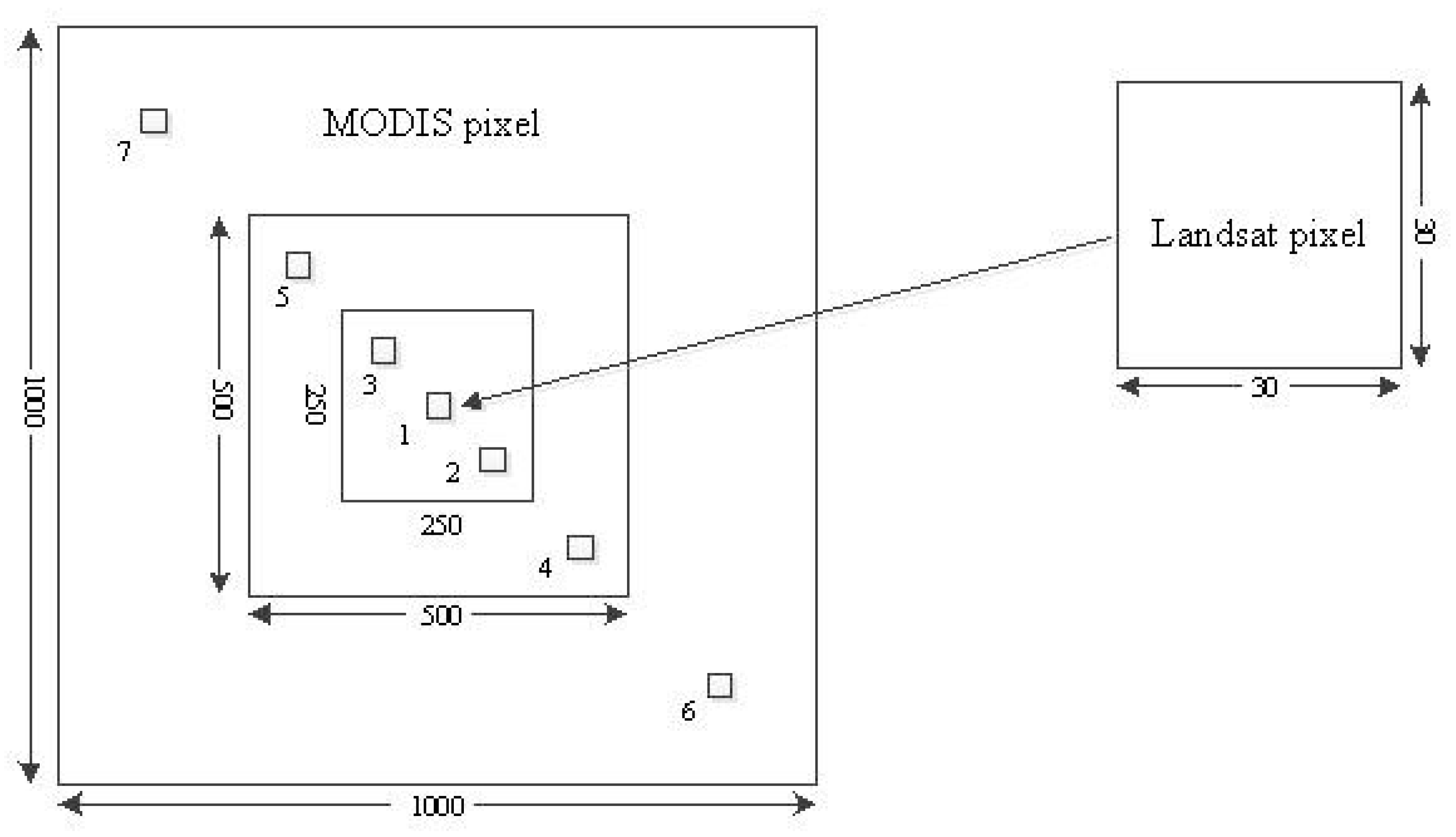The inconsistency of spatial resolutions between sample plot and remotely sensed data will result in a great challenge for mapping and accuracy assessment of forest carbon density [11,20,27,31,32,33,34,35]. There have only been few relevant studies reported in this field. For this purpose, in this study, a methodological framework was proposed and tested by developing a systematical, nested and clustering sampling design to collect reference data, then generating maps of forest carbon density and conducting accuracy assessment of the maps at four spatial resolutions for Huang-Feng-Qiao forest farm of You County in Eastern Hunan of China. In the sampling design, the used sample plots had a size of 30 m × 30 m. A systematical and equal sampling distance was used to select the 250 m and 500 m sub-blocks and 1000 m blocks. The 30 m sample plots, and 250 m and 500 m sub-blocks were nested within the 1000 m blocks. The sample plots that formed clusters were systematically and consistently allocated along the diagonal lines of the sub-blocks and blocks with unequal, but fixed distances. There were several reasons for using this sampling design. First, most national forest inventories, for example, the national forest inventory in China, use systematical sampling designs and thus the developed methodology can be directly applied to generate forest carbon density maps with the existing national forest inventory sample plots. Second, the four used spatial resolutions: 30 m × 30 m, 250 m × 250 m, 500 m × 500 m and 1000 m × 1000 m match the pixel sizes of the widely used Landsat image and three MODIS products respectively. Third, a certain number of sample plots instead of all of the sample units within the sub-blocks and blocks were selected and measured to make reference of forest biomass and carbon density at the sub-block and block levels to reduce the cost of collecting field plot data. Moreover, a random sampling is not widely used for national forest inventory. In addition, a double and systematical sampling based on stratification and combined with nested sub-blocks with clusters of sample plots may be more efficient, but much more complicated and thus more difficult to use compared to this sampling design.

In addition to the 30 m spatial resolution sample plots, this multi-resolution sampling design led to three, five and seven sample plots for each of the 250 m sub-blocks, 500 m sub-blocks and 1000 m blocks to capture the variation of forest carbon density, respectively. To save time and reduce cost, not all of the 30 m sample plots were measured within each of the sub-blocks and blocks. Instead, three, five and seven sample plots were selected and measured, and an average value from the sample plots was utilized to make the reference of forest carbon density for each of the 250 m sub-blocks, 500 m sub-blocks and 1000 m blocks. This would have resulted in uncertainties of forest carbon density values at the sub-block and block levels. However, this study focused on proposing an idea and developing a methodological framework for multi-resolution mapping and accuracy assessment of forest carbon density and thus, using the numbers of the sample plots would not affect the conclusions of this study. Whether the numbers of sample plots selected at the sub-block and block levels are enough and optimal should be further analyzed in the further studies. In fact, the optimal number of sample plots for each of the coarse spatial resolutions may vary depending on the complexity of forest ecosystems and geographic features [50].

This study area had a complicated and fragmented forest landscape where various mixed forests, scattered bamboo forests and shrubs, and agricultural lands exist. A relatively large CV (106%) of forest carbon density was obtained from the 30 m spatial resolution sample plots. As expected, the CV greatly decreased from the plot level to the sub-block and block levels. The results of this study showed that although all of the means of the predicted values and maps fell in the confidence intervals of the reference data at the corresponding spatial resolutions, the obtained forest carbon density maps had a larger value (34%)of relative RMSE at the 30 m resolution plot level compared to the previous studies [11,20,32,34]. For example, Bastin et al. [34] combined fine spatial resolution satellite images, harmonizing Fourier textural ordination and piecewise biomass inversion models based on 26 inventory plots (1 ha) to predict AGB in Central Africa. They obtained an accuracy of residual standard error (RSE) 15% for forest AGB predictions at the spatial resolution of 100 m × 100 m across a wide range of 26 Mg/ha to 460 Mg/ha by cross validation. Moreover, Asner et al. [32] used a top-down approach to scale up high spatial resolution carbon estimates to a large region of 16.5 million ha in the Colombian Amazon. They yielded an uncertainty of 14% for LiDAR-derived carbon maps at 1 ha resolution and an uncertainty of 28% for the regional map based on stratification. Compared to those in the studies of Bastin et al. [34] and Asner et al. [32], however, in this study the used sample plots and map units were smaller, while the spatial resolution of the used Landsat image was coarser. In addition, other reasons may include more complicated and fragmented forest landscape, the larger CV and neglecting environmental variables and stratification of the landscape. This implied that considering environmental variables and stratification of landscapes and using finer spatial resolution images may provide the potential of increasing the accuracy of mapping forest carbon density. On the other hand, in this study, the accuracy of forest carbon density at the plot level was only slightly lower than that (28%) from the study of Guitet et al. [33] at the similar plot scale, but much higher than that (53%) for the use of Landsat imagery by Fu et al. [11] in which an upscaling method that combines footprint climatology modeling, modified regression tree and image fusion was utilized to estimate net ecosystem exchange.

In this study, when the 30 m spatial resolution Landsat 8 image and sample plot data were scaled up to the pixel sizes of 250 m × 250 m, 500 m × 500 m and 1000 m × 1000 m using both algorithm SGCSWA and SGBCS, the obtained relative RMSEs of forest carbon density estimates varied from 5.45% to 5.92%. At the corresponding spatial resolutions the combinations of MODIS products and the reference data led to a range of relative RMSEs from 6.38% to 6.70%. The accuracies at the sub-block and block levels were much higher than that at the plot level mainly because of the smoothing of spatial data and consideration of the features of clustering sampling. The accuracies were also much higher than those (53% vs. 46% for Landsat and MODIS imagery, respectively) from the study of Fu et al. [11]. Compared to the previous reports [11,32,33,34], this study has an advantage. That is, a multi-resolution sampling design was developed and from which multi-resolution reference datasets that match the spatial resolutions of the most widely used Landsat and MODIS images were obtained and can be used to conduct mapping and accuracy assessment of forest carbon density. Moreover, the algorithms can scale up both spatial data and input uncertainties and generate the maps of estimates and their uncertainties at coarser spatial resolutions. However, the algorithms require intensive computation for very large areas. This limitation has become less critical as computer science develops. In addition, in this study, only 3–7 30 m spatial resolution sample plots (not all of the sample units) were measured within each of the sub-blocks and blocks, which may have resulted in uncertainties of forest carbon density predictions. Readers should take caution for use of the results and further studies are needed.

This study also showed that the combination of Landsat 8 image and the algorithm SGCSWA resulted in the greatest accuracies of the up-scaled maps, then the combination of Landsat 8 image and SGBCS, and the combinations of the MODIS images and SGCS had lowest accuracies. The reason is mainly because the medium spatial resolution Landsat 8 image provides more detailed information of forest carbon density than the coarser spatial resolution MODIS products. Both algorithms SGCSWA and SGBCS can combine and scale up the 30 spatial resolution sample plot and image data to produce any coarser spatial resolution forest carbon density maps and eliminate the requirement of collecting plot data at the coarser spatial resolutions. Instead of MODIS images, thus, the medium spatial resolution Landsat image with both up-scaling algorithms SGCSWA and SGBCS is recommended for mapping and accuracy assessment of forest carbon density at the coarser spatial resolutions.

It has to be pointed out that in this study, we calculated many band ratios, vegetation indices and texture measures to capture the forest canopy structures and spatial heterogeneity and reduce the effects of slope due to mountainous areas. However, in these algorithms (SGCSWA and SGBCS), only the spectral variable that had the greatest correlation with forest carbon density for each of the spatial resolutions was utilized. The spatial variability of forest carbon density was thus limitedly explained, which may also have increased the uncertainty of predicted values. In future studies, especially when these algorithms are applied to mapping forest carbon density of complicated rainforests, more spectral variables should be used to conduct the co-simulations. This will require a spatial joint multivariate co-simulation algorithm. This method is more complicated and will double the computation and labor costs [51]. However, the development of computer science will release this limitation.

Finally, in this study, we explored the mapping of forest carbon density at the spatial resolutions of 30 m, 250 m, 500 m and 1000 m instead of other spatial resolutions such as 90 m. There were three reasons for selecting these four spatial resolutions. First, the spatial resolutions exactly match the pixel sizes of Landsat 8 image and three MODIS products that are widely used to map forest carbon density at local, regional, national and global scales. Second, Wang et al. [27] conducted the up-scaling of spatial data from a spatial resolution of 30 m × 30 m to 90 m × 90 m for mapping vegetation cover using the SGBCS and testified the success of this up-scaling algorithm. Moreover, the purpose of this study was to demonstrate the development of a general methodological framework for mapping forest carbon density at multiple spatial resolutions and the obtained conclusions would be thus generalized.

5. Conclusions

This study focused on the development and assessment of a methodology to conduct mapping and accuracy assessment of forest carbon density at four spatial resolutions by combining Landsat 8 and MODIS images with reference values from sample plots obtained using a multiple resolution, systematical, nested and clustering sampling design. As expected, the results of applying the methodology to the study area showed that all of the means of predicted forest carbon density values at the spatial resolutions of 30 m × 30 m, 250 m × 250 m, 500 m × 500 m and 1000 m × 1000 m fell in the confidence intervals of reference data at a significance level of 0.05. Moreover, with the same reference datasets, images, and the methods, as the spatial resolutions became coarser, the accuracy of the up-scaled predictions decreased and the maps became smoothed. More important is that this study led to four new conclusions. First, the systematical, nested and clustering sampling design provided the potential to obtain spatial information of forest carbon density at multiple spatial resolutions. Second, the relative RMSEs of predicted values at the plot level were much greater than those at the sub-block and block levels. Moreover, the accuracies of the up-scaled estimates were much higher than those from previous studies. In addition, at the same spatial resolution, SGCSWA resulted in smallest relative RMSEs of the up-scaled predictions, then the combinations of Landsat image and SGBCS, and the accuracies from both methods were significantly greater than those from the combinations of the MODIS images and SGCS. Overall, this study implied that the combinations of Landsat 8 image and SGCSWA or SGBCS with the systematical, nested and clustering sampling design provided the potential to formulate a methodological framework to map forest carbon density and conduct accuracy assessment at multiple spatial resolutions. However, this methodology needs to be further refined and examined in other forest landscapes.

References

1. Cartus, O.; Kellndorfer, J.; Walker, W.; Franco, C.; Bishop, J.; Santos, L.; Michel Fuentes, J.M. A National, Detailed Map of Forest Aboveground Carbon Stocks in Mexico. Remote Sens. 2014, 6, 5559–5588. [Google Scholar] [CrossRef]
2. Intergovernmental Panel on Climate Change (IPCC). Climate Change 2007: The Physical Science Basis: Working Group I Contribution to the Fourth Assessment Report of the IPCC; Cambridge University Press: Cambridge, UK, 2007. [Google Scholar]
3. Houghton, R.A. Aboveground forest biomass and the global carbon balance. Glob. Chang. Biol. 2005, 11, 945–958. [Google Scholar] [CrossRef]
4. Zhou, X.; Peng, C.; Dang, Q.; Chen, J.; Parton, S. A simulation of temporal and spatial variations in carbon at landscape level: A case study for Lake Abitibi Model Forest in Ontario, Canada. Mitig. Adapt. Strateg. Glob. Chang. 2007, 12, 525–543. [Google Scholar] [CrossRef]
5. Main-Knorn, M.; Moisen, G.G.; Healey, S.P.; Keeton, W.S.; Freeman, E.A.; Hostert, P. Evaluating the remote sensing and inventory-based estimation of biomass in the Western Carpathians. Remote Sens. 2011, 3, 1427–1446. [Google Scholar] [CrossRef]
6. Attarchi, S.; Gloaguen, R. Improving of above groud biomass using dual polarimetric PALSAR and ETM+ data in the Hyrcanian fore tainnuomts (Iran). Remote Sens. 2014, 6, 3693–3715. [Google Scholar] [CrossRef]
7. Tian, X.; Su, Z.; Chen, E.; Li, Z.; Tol, C.; Guo, J.; He, Q. Estimation of forest above-ground biomass using multi-parameter remote sensing data over a cold and arid area. Int. J. Appl. Earth Obs. Geoinf. 2012, 14, 160–168. [Google Scholar] [CrossRef]
8. Powell, S.L.; Cohen, W.B.; Healey, S.P.; Kennedy, R.E.; Moisen, G.G.; Pierce, K.B.; Ohmannb, J.L. Quantification of live aboveground forest biomass dynamics with Landsat time-series and field inventory data: A comparison of empirical modeling approaches. Remote Sens. Environ. 2010, 114, 1053–1068. [Google Scholar] [CrossRef]
9. Lu, D.; Chen, Q.; Wang, G.; Liu, L.; Moran, E. A Survey of Remote Sensing-Based Aboveground Biomass Estimation Methods. Int. J. Digit. Earth 2016, 9, 63–105. [Google Scholar] [CrossRef]
10. Fang, J.; Chen, A.; Peng, C.; Zhao, S.; Ci, L. Changes in forest biomass carbon storage in China between 1949 and 1998. Science 2002, 292, 2320–2322. [Google Scholar] [CrossRef] [PubMed]
11. Fu, D.; Chen, B.; Zhang, H.; Wang, J.; Black, A.; Amiro, B.D. Estimating landscape net ecosystem exchange at high spatial–temporal resolution based on Landsat data, an improved upscaling model framework, and eddy covariance flux measurements. Remote Sens. Environ. 2014, 141, 90–104. [Google Scholar] [CrossRef]
12. Landsberg, J.J.; Waring, R.H. A generalized model of forest productivity using simplified concepts of radiation-use efficiency, carbon balance, and partitioning. For. Ecol. Manag. 1997, 95, 209–228. [Google Scholar] [CrossRef]
13. Running, S.W.; Hunt, E.R., Jr. Generalization of a forest ecosystem process model for other biomes, BIOME-BGC, and an application for global scale models. In Scaling Physiological Processes: Leaf to Globe; Ehleringer, J.R., Field, C.B., Eds.; Academic Press, Inc.: San Diego, CA, USA, 1993; pp. 141–158. [Google Scholar]
14. Phutchard, V.; Rajendra, P.S.; Masahiko, N.; Abdul, P.S.; Somboon, K. Carbon stock assessment using remote sensing and forest inventory data in Savannakhet, Lao PDR. Remote Sens. 2014, 6, 5452–5479. [Google Scholar]
15. Kankare, V.; Vastaranta, M.; Holopainen, M.; Raty, M.; Yu, X.; Hyyppa, J.; Hyyppa, H.; Alho, P.; Viitala, R. Retrieval of forest aboveground biomass and stem volume with airborne scanning LiDAR. Remote Sens. 2013, 5, 2257–2274. [Google Scholar] [CrossRef] [Green Version]
16. Vicharnakorn, P.; Shrestha, R.P.; Nagai, M.; Salam, A.P.; Kiratiprayoon, S. Carbon Stock Assessment Using Remote Sensing and Forest Inventory Data in Savannakhet, Lao PDR. Remote Sens. 2014, 6, 5452–5479. [Google Scholar] [CrossRef]
17. Robinson, C.; Saatchi, S.; Neumann, M.; Gillespipe, T. Impacts of spatial variability on aboveground biomass estimation from L-band Radar in a temperate forest. Remote Sens. 2013, 5, 1001–1023. [Google Scholar] [CrossRef]
18. Yan, E.; Lin, H.; Wang, G.; Sun, H. Improvement of forest carbon estimation by integration of regression modeling and spectral unmixing of Landsat data. IEEE Geosci. Remote Sens. Lett. 2015, 12, 2003–2007. [Google Scholar]
19. Fleming, A.; Wang, G.; McRoberts, R. Comparison of methods toward multi-scale forest carbon mapping and spatial uncertainty analysis: Combining national forest inventory plot data and Landsat TM images. Eur. J. For. Res. 2015, 134, 125–137. [Google Scholar] [CrossRef]
20. Wang, G.; Oyana, T.; Zhang, M.; Adu-prah, S.; Zeng, S.; Lin, H.; She, J. Mapping and spatial uncertainty analysis of forest vegetation carbon by combining national forest inventory data and satellite images. For. Ecol. Manag. 2009, 258, 1275–1283. [Google Scholar] [CrossRef]
21. Lu, D. The potential and challenge of remote sensing-based biomass estimation. Int. J. Remote Sens. 2006, 27, 1297–1328. [Google Scholar] [CrossRef]
22. McRoberts, R.E.; Tomppo, E.O.; Finley, A.O.; Heikkinen, J. Estimating areal means and variances of forest attributes using the k-Nearest Neighbors technique and satellite imagery. Remote Sens. Environ. 2007, 111, 466–480. [Google Scholar] [CrossRef]
23. Shvidenko, A.; Schepaschenko, D.; Nilsson, S.; Bouloui, Y. Semi-empirical models for assessing biological productivity of Northern Eurasian forests. Ecol. Model. 2007, 204, 163–179. [Google Scholar] [CrossRef]
24. Wagner, F.; Rutishauser, E.; Blanc, L.; Herault, B. Effects of Plot Size and Census Interval on Descriptors of Forest Structure and Dynamics. Biotropica 2010, 42, 664–671. [Google Scholar] [CrossRef]
25. Réjou-Méchain, M.; Muller-Landau, H.C.; Detto, M.; Thomas, S.C.; Le Toan, T.; Saatchi, S.S.; Barreto-Silva, J.S.; Bourg, N.A.; Bunyavejchewin, S.; Butt, N.; et al. Local spatial structure of forest biomass and its consequences for remote sensing of carbon stocks. Biogeosci. Discuss. 2014, 11, 5711–5742. [Google Scholar] [CrossRef]
26. Gertner, G.Z.; Wang, G.; Anderson, A.B.; Howard, H. Combining stratification and up-scaling method-block cokriging with remote sensing imagery for sampling and mapping an erosion cover factor. Ecol. Inf. 2007, 2, 373–386. [Google Scholar] [CrossRef]
27. Wang, G.; Gertner, G.Z.; Anderson, A.B. Spatial variability based algorithms for scaling up spatial data and uncertainties. IEEE Trans. Geosci. Remote Sens. 2004, 42, 2004–2015. [Google Scholar] [CrossRef]
28. Marceau, D.J. The scale issue in social and natural sciences. Can. J. Remote Sens. 1999, 25, 347–356. [Google Scholar] [CrossRef]
29. Marceau, D.J.; Hay, G.J. Remote sensing contributions to the scale issue. Can. J. Remote Sens. 1999, 25, 357–366. [Google Scholar] [CrossRef]
30. Wang, G.; Gertner, G.Z.; Anderson, A.B. Up-scaling methods based on variability-weighted and simulation for inferring spatial information cross scales. Int. J. Remote Sens. 2004, 25, 4961–4979. [Google Scholar] [CrossRef]
31. Wang, G.; Zhang, M. Upscaling with conditional co-simulation for mapping aboveground forest carbon. In Scale Issue in Remote Sensing; Weng, Q., Ed.; John Wiley and Sons: Hobboken, NJ, USA, 2014; pp. 108–125. [Google Scholar]
32. Asner, G.P.; Clark, J.K.; Mascaro, J.; Galindo García, G.A.; Chadwick, K.D.; Navarrete Encinales, D.A.; Paez-Acosta, G.; Cabrera Montenegro, E.; Kennedy-Bowdoin, T.; Duque, Á.; et al. High-resolution mapping of forest carbon stocks in the Colombian Amazon. Biogeosciences 2012, 9, 2683–2696. [Google Scholar] [CrossRef]
33. Guitet, S.; Herault, B.; Molto, Q.; Brunaux, O.; Couteron, P. Spatial structure of above-ground biomass limits accuracy of carbon Mapping in Rainforest but Large Scale Forest Inventories Can Help to Overcome. PLoS ONE 2015, 10. [Google Scholar] [CrossRef] [PubMed] [Green Version]
34. Bastin, J.; Barbier, N.; Couteron, P.; Admas, B.; Shapiro, A.; Bogaert, J.; Canniere, C.D. Aboveground biomass mapping of African forest mosaics using canopy texture analysis: Toward a regional approach. Ecol. Appl. 2014, 24, 1984–2001. [Google Scholar] [CrossRef]
35. Wang, G.; Gertner, G.Z. Spatial uncertainty analysis when mapping natural resources using remotely sensed data. In Remote Sensing of Natural Resources; Wang, G., Weng, Q., Eds.; CRC Press, Taylor & Francis Group: Boca Raton, FL, USA, 2013; pp. 87–107. [Google Scholar]
36. Huber, M.O.; Eastaugh, C.S.; Gschwantner, T.; Hasenauer, H.; Kindermann, G.; Ledermann, T.; Lexer, M.J.; Rammera, W.; Schörghuber, S.; Sterba, H. Comparing simulations of three conceptually different forest models with National Forest Inventory data. Environ. Model. Softw. 2013, 40, 88–97. [Google Scholar] [CrossRef]
37. Hulsman, L.L.; Garrick, D.J.; Gill, C.A.; Herring, A.D.; Sanders, J.O.; Riley, D.G. Cross-validation of genetic and genomic predictions of temperament in Nellore–Angus crossbreds. Livestock Sci. 2015, 182, 28–33. [Google Scholar] [CrossRef]
38. Wong, T.T. Performance evaluation of classification algorithms by k-fold and leave-one-out cross validation. Pattern Recogn. 2015, 48, 2839–2846. [Google Scholar] [CrossRef]
39. Larocque, G.R.; Bhatti, J.S.; Boutin, R.; Chertov, O. Uncertainty analysis in carbon models of forest ecosystems: Research needs and development of a theoretical framework to estimate error propagation. Ecol. Model. 2008, 219, 400–412. [Google Scholar] [CrossRef]
40. Chen, Q.; Laurin, G.V.; Valentini, R. Uncertainty of remotely sensed aboveground biomass over an African tropical forest: Propagating errors from trees to plots to pixels. Remote Sens. Environ. 2015, 150, 134–143. [Google Scholar] [CrossRef]
41. Nabuurs, G.J.; van Putten, B.; Knippers, T.S.; Mohren, G.M.J. Comparison of uncertainties in carbon sequestration estimates for a tropical and a temperate forest. For. Ecol. Manag. 2008, 256, 237–245. [Google Scholar] [CrossRef]
42. Yan, E. Study on Extraction of Broad-leaved Forest Information Based on Medium and High Spatial Resolution Remote Sensing Image; Master Degree Thesis of Central South University of Forestry & Technology: Changsha, China, 2011. [Google Scholar]
43. Li, H. Estimation and Evaluation of Forestry Biomass Carbon Storage in China; China Forestry Press: Beijing, China, 2011; pp. 30–31, 58. [Google Scholar]
44. Wu, D.; Shao, Q.; Liu, J.; Huang, L. Spatio temporal dynamics of forest carbon storage in Taihe County of Jiangxi Province in 1985–2030. Chinese J. Appl. Ecol. 2011, 22, 41–46. [Google Scholar]
45. Xiang, H.; Liu, J.; Cao, C.; Xu, M. Algorithms for moderate resolution imaging spectroradiometer cloud-free image compositing. J. Appl. Remote Sens. 2013, 7, 073486. [Google Scholar] [CrossRef]
46. Song, X.; Li, J. Technologies for Sampling and Inventory, 2rd ed.; Chinese Forestry Press: Beijing, China, 2007. [Google Scholar]
47. Deutsch, C.V.; Journel, A.G. Geostatistical Software Library and User’s Guide; Oxford University Press: New York, NY, USA, 1998. [Google Scholar]
48. Wang, G.; Gertner, G.Z.; Anderson, A.B.; Howard, H.R. Repeated measurements on permanent plots using local variability based sampling for monitoring soil erosion. Catena 2008, 73, 75–88. [Google Scholar] [CrossRef]
49. Pineiro, G.; Perelman, S.; Guerschman, J.P.; Paruelo, J.M. How to evaluate models: Observed vs. predicted or predicted vs. observed? Ecol. Model. 2008, 216, 316–322. [Google Scholar] [CrossRef]
50. Zhang, M.; Wang, G.; Zhou, G.; Ge, H.; Xu, L.; Zhou, Y. Mapping of forest carbon by combining forest inventory data and satellite images with co-simulation based up-scaling method. Acta Ecol. Sin. 2009, 29, 2919–2928. [Google Scholar]
51. Gertner, G.; Wang, G.; Fang, S.; Anderson, A.B. Mapping and uncertainty of predictions based on multiple primary variables from joint co-simulation with TM image. Remote Sens. Environ. 2002, 83, 498–510. [Google Scholar] [CrossRef]
Figure 1. The location of the study area, Huang-Feng-Qiao forest farm of You county in Eastern Hunan of China (top left); and its color infrared composite image of Landsat 8 with the spatial distributions of 1000 m × 1000 m sample blocks and 30 m × 30 m sample plots within each block (bottom).
Remotesensing 08 00571 g001
Figure 2. Allocation of 30 m × 30 m spatial resolution sample plots along the diagonal line within each of 1000 m × 1000 m blocks where in addition to a 30 m × 30 m sample plot, two sub-blocks of 250 m × 250 m and 500 m × 500 m were nested.
Remotesensing 08 00571 g002
Figure 3. (a) Image-based sequential Gaussian co-simulation (SGCS); and (b) block co-simulation (SGBCS) algorithms (cross symbol indicates sample plots and pixel u was predicted).
Remotesensing 08 00571 g003
Figure 4. The residuals against the predicted values of forest carbon density for the maps at the spatial resolution of: (a) 30 m × 30 m using sequential Gaussian co-simulation (SGCS); and at the spatial resolutions of: (b) 250 m × 250 m; (c) 500 m × 500 m; and (d) 1000 m × 1000 m using SGCSWA (scaling up the predicted values of the above 30 m spatial resolution map from SGCS to the coarser spatial resolutions with a window average method (WA)).
Remotesensing 08 00571 g004
Figure 5. Spatial distributions of: (a) predicted forest carbon density values at the spatial resolution of 30 m × 30 m by combining Landsat 8 image and sample plot data using sequential Gaussian co-simulation (SGCS); and (b) the variances of the predicted values.
Remotesensing 08 00571 g005
Figure 6. Spatial distributions of predicted forest carbon density values at the spatial resolutions of: (a) 250 m × 250 m; (b) 500 m × 500 m; and (c) 1000 m × 1000 m by combining and scaling up Landsat 8 image and sample plot data using sequential Gaussian block co-simulation (SGBCS).
Remotesensing 08 00571 g006
Figure 7. Spatial distributions of predicted forest carbon density values by combining MODIS products and the reference values from the sample plots within the sub-blocks and blocks using sequential Gaussian co-simulation (SGCS) at the spatial resolutions of: (a) 250 m × 250; (b) 500 m × 500 m; and (c) 1000 m × 1000 m.
Remotesensing 08 00571 g007