
Fast Binary Coding for the Scene Classification of High-Resolution Remote Sensing Imagery


Abstract
:
1. Introduction
- -
- We develop a fast global feature representation method for image scenes, named fast binary coding (FBC), which integrates the local feature extraction and feature coding stage. In the FBC pipeline, we are free of any hand-crafted features, and the features are skillfully learned and encoded in an unsupervised fashion.
- -
- We achieve promising performance with extraordinarily low computational efficiency on scene classification of HRRS images, which can make the FBC an effective and practical method for an industrial scene analysis system.
- -
- On the basis of FBC, we investigate how the spatial kernel extension and various saliency maps can improve the classification performance.
2. Related Work
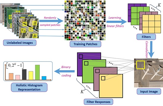
3. Fast Binary Coding For Scene Classification
3.1. Fast Binary Coding
3.2. Analysis of the Computational Complexity of FBC
- -
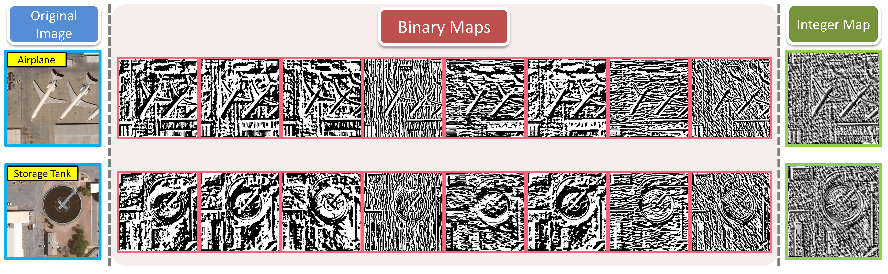
- Convolving an image scene with filters is a linear operation;
- -
- Binarizing the filter responses is a thresholding operation;
- -
- Converting binary maps to the integer map is a linear operation according to Equation (4);
- -
- Obtaining the histogram features only needs to count the frequency of integers within .
3.3. Scene Classification
| Algorithm 1 FBC-based scene classification framework. |
| Input: |
|
| Output: |
| The predicted labels for testing image scenes, ; |
|
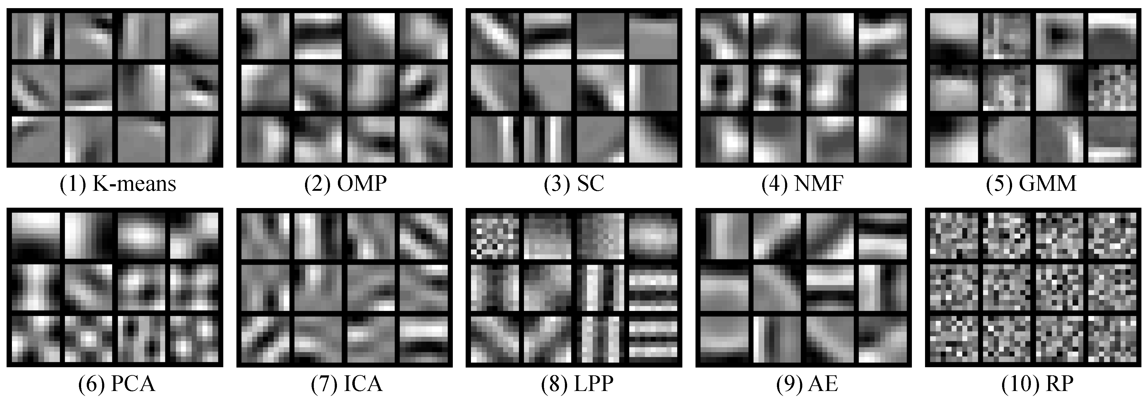
3.4. Learning via Unsupervised Learning Methods
- -
- Randomly extract a large number of S image patches with size of from the training image dataset;
- -
- Normalize each patch to zero mean and unit variance.
3.4.1. K-Means Clustering
3.4.2. Orthogonal Matching Pursuit
3.4.3. Sparse Coding
3.4.4. Non-Negative Matrix Factorization
3.4.5. Gaussian Mixture Model
3.4.6. Principal Component Analysis
3.4.7. Locality-Preserving Projection
3.4.8. Auto-Encoder
4. Extensions to FBC
- FBC lacks sufficient representative power to depict the spatial layout information of image scenes;
- FBC counts all of the codewords to construct the histogram feature, whereas some of the codewords are probably not helpful to the descriptive ability of histogram features and even have a negative influence on the final classification performance.
4.1. Spatial Co-Occurrence Kernel
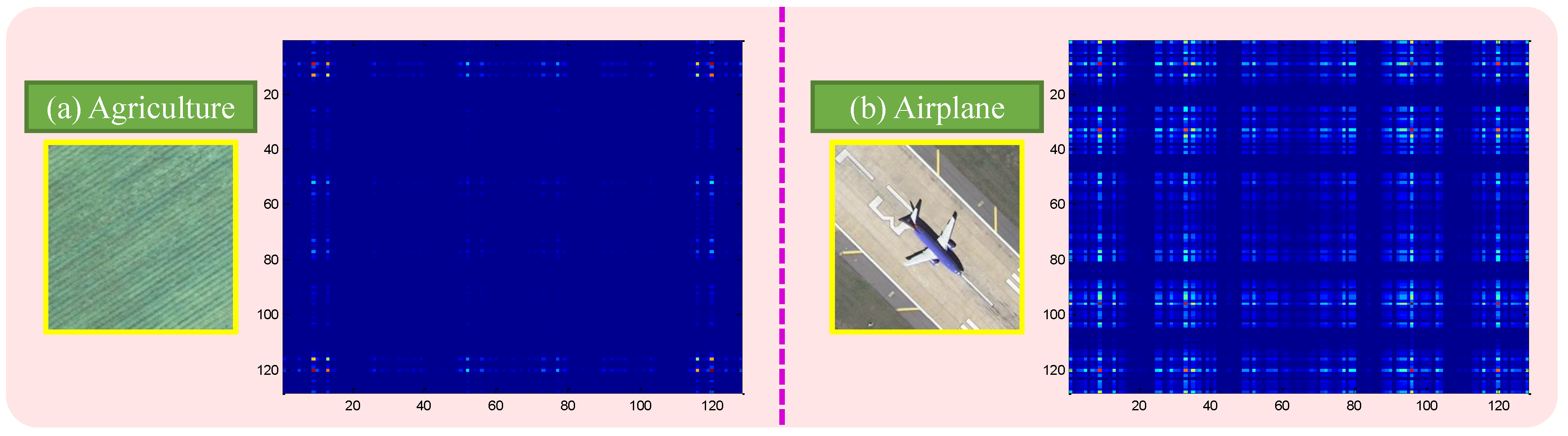
4.2. Feature Coding Based on the Saliency Map
5. Experiments and Analysis
5.1. Experimental Setup
- -
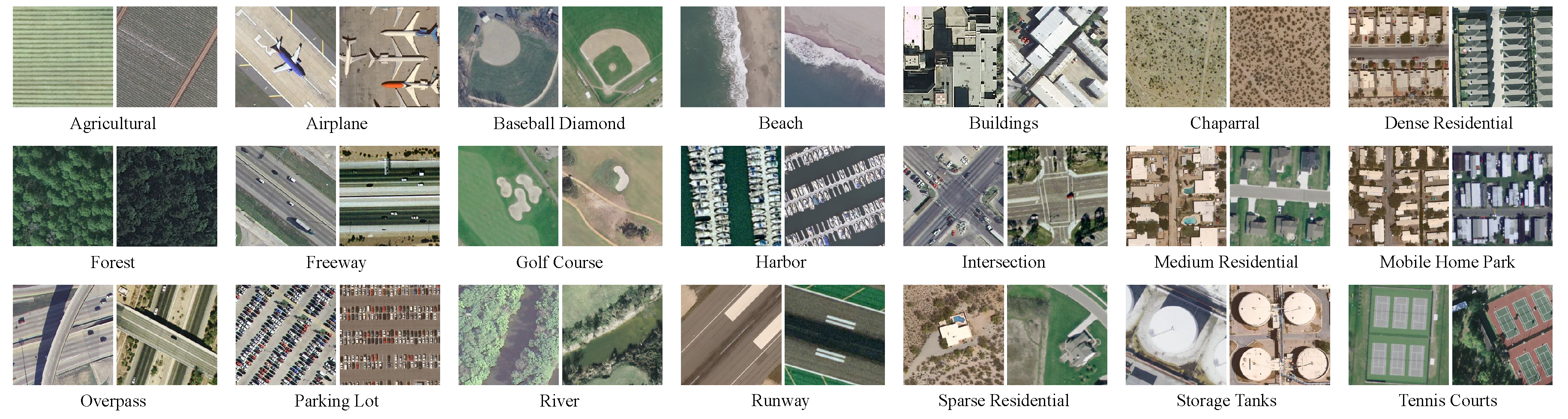
- UC Merced Land Use Dataset. The UC Merced dataset (UCM) [32] contains 21 typical scene categories, each of which consists of 100 images with a size of 256 × 256 pixels. Figure 7 shows two examples of each class included in this dataset. This dataset shows very small inter-class diversity among some categories that share a few similar objects or textural patterns (e.g., dense residential and medium residential), which leads the UCM dataset to be a challenging one.
- -
- WHU-RS Dataset. The WHU-RSdataset [4] is a new publicly-available dataset, which consists of 950 images with a size of 600 × 600 pixels uniformly distributed in 19 scene classes. All images are collected from Google Earth (Google Inc.). Some example images are shown in Figure 8. We can see that the variation of illumination, scale, resolution and viewpoint-dependent appearance makes each scene category more complicated than the UCM dataset.
5.2. Experimental Results
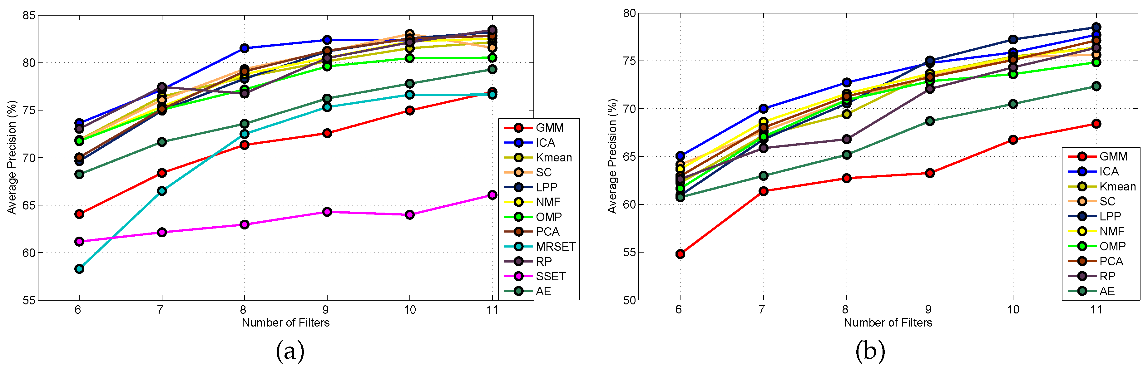
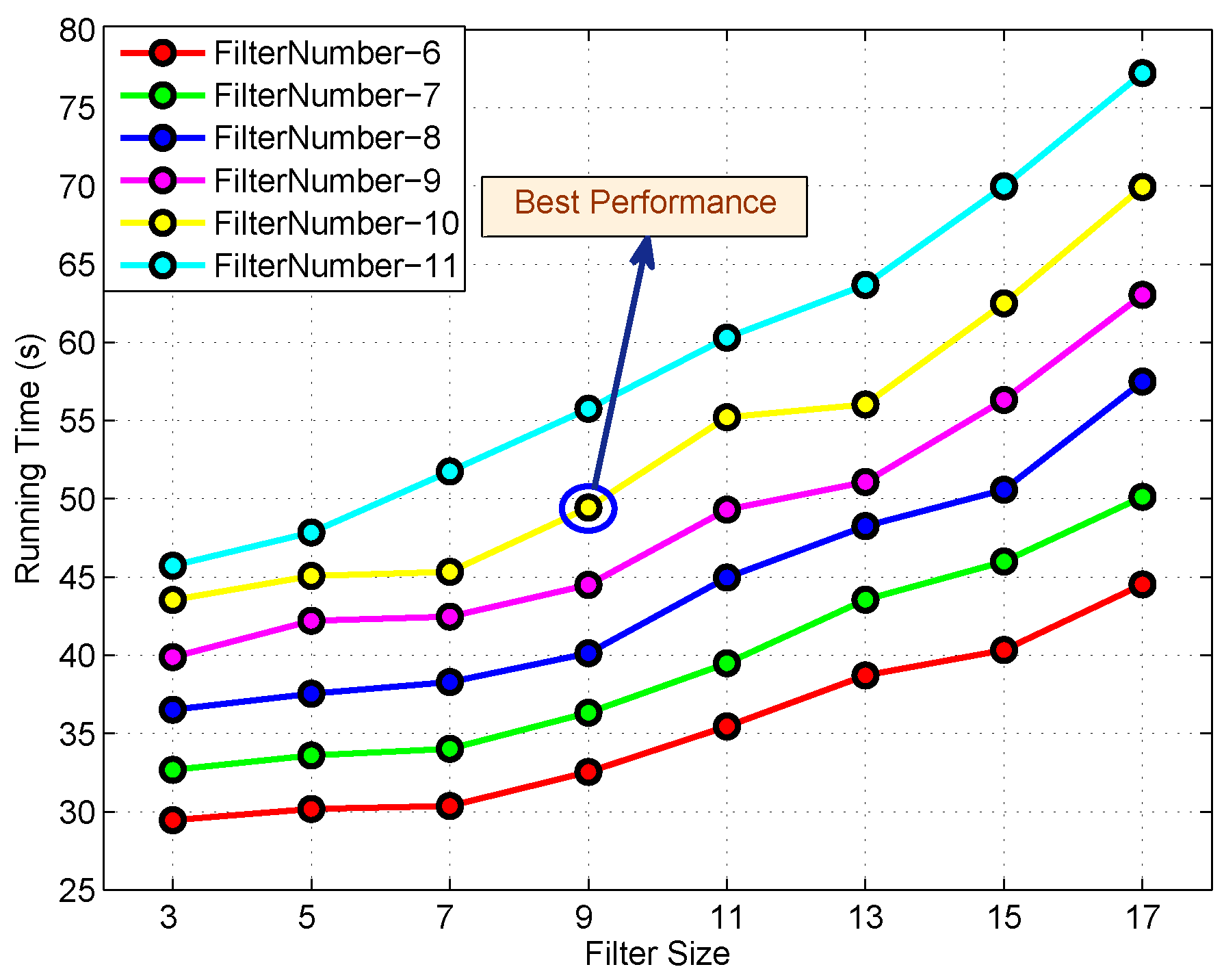
5.2.1. Results of FBC
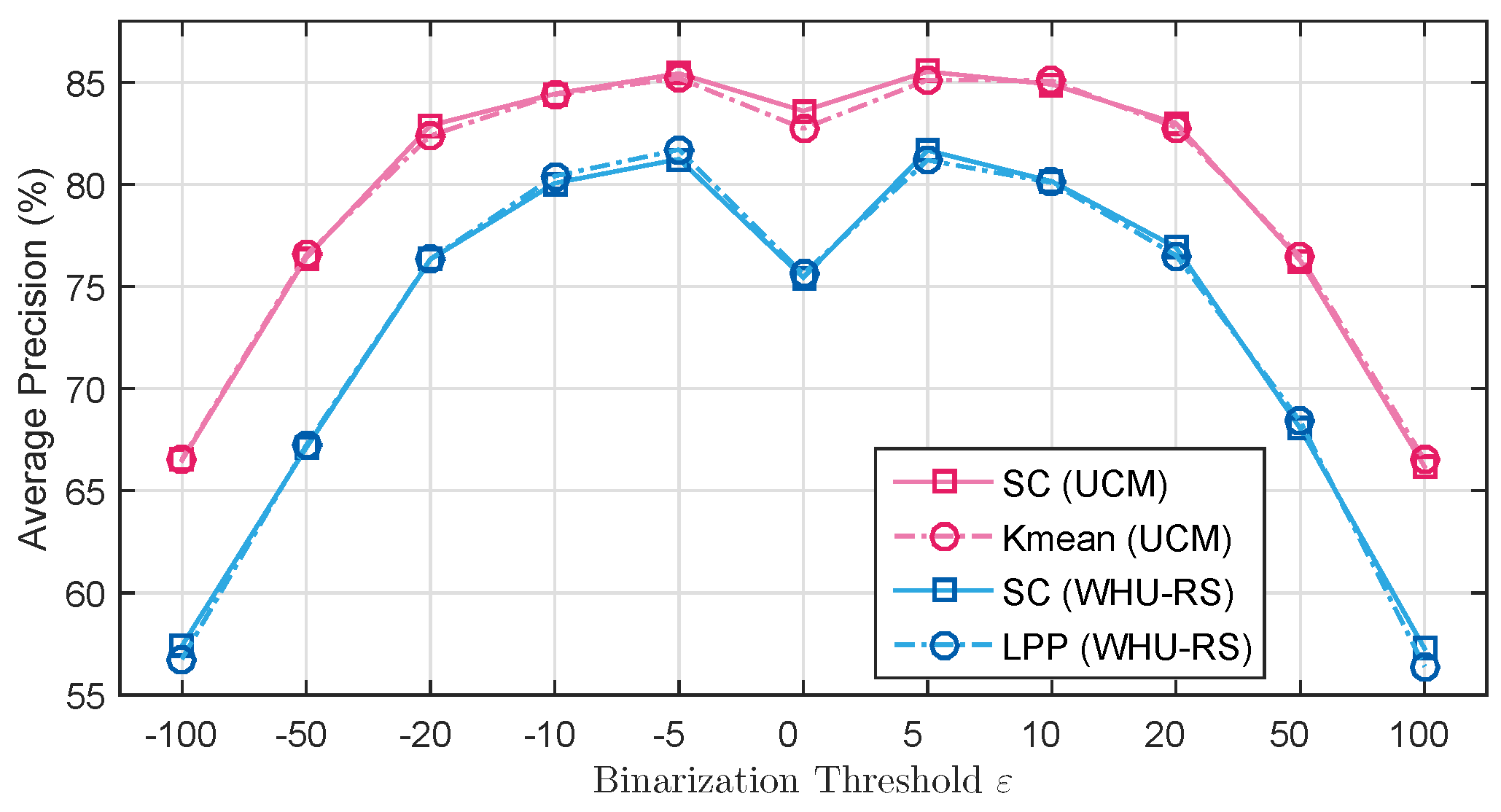
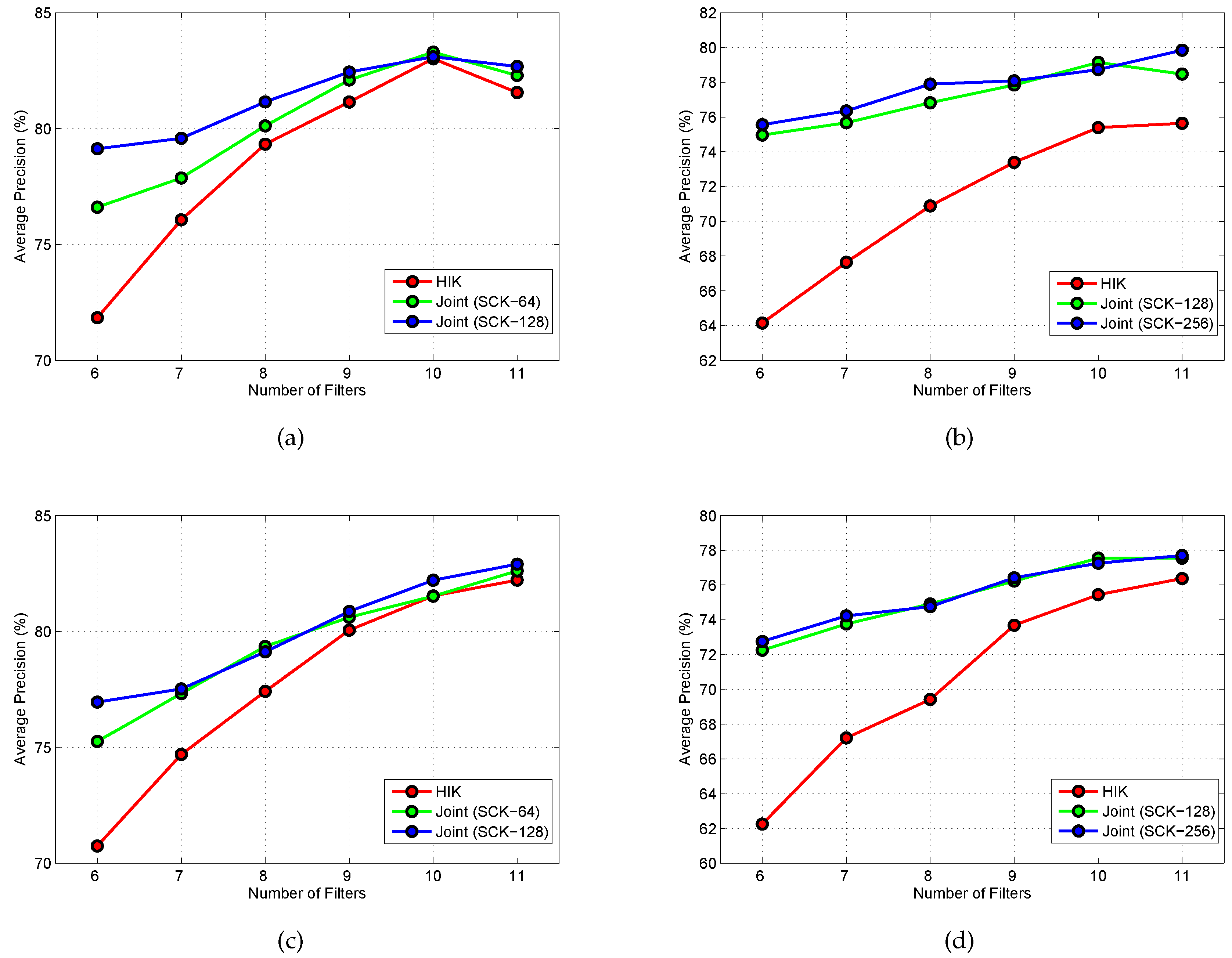
5.2.2. Results of SCK
5.2.3. Results of Saliency-Based Coding
6. Discussion
7. Conclusions
Acknowledgments
Author Contributions
Conflicts of Interest
References
- Li, D.; Zhang, L.; Xia, G.S. Automatic analysis and mining of remote sensing big data. Acta Geod. Cartogr. Sin. 2014, 43, 1211–1216. [Google Scholar]
- Rathore, M.M.U.; Paul, A.; Ahmad, A.; Chen, B.W.; Huang, B.; Ji, W. Real-Time Big Data Analytical Architecture for Remote Sensing Application. IEEE J. Sel. Top. Appl. Earth Obs. Remote Sens. 2015, 8, 4610–4621. [Google Scholar] [CrossRef]
- Christophe, E.; Michel, J.; Inglada, J. Remote Sensing Processing: From Multicore to GPU. IEEE J. Sel. Top. Appl. Earth Obs. Remote Sens. 2011, 4, 643–652. [Google Scholar] [CrossRef]
- Xia, G.S.; Yang, W.; Delon, J.; Gousseau, Y.; Sun, H.; Maitre, H. Structrual High-Resolution Satellite Image Indexing. In Proceedings of the ISPRS, TC VII Symposium (Part A): 100 Years ISPRS—Advancing Remote Sensing Science, Vienna, Austria, 5–7 July 2010.
- Lienou, M.; Maitre, H.; Datcu, M. Semantic annotation of satellite images using latent dirichlet allocation. IEEE Geosci. Remote Sens. Lett. 2010, 7, 28–32. [Google Scholar] [CrossRef]
- Cheriyadat, A. Unsupervised Feature Learning for Aerial Scene Classification. IEEE Trans. Geosci. Remote Sens. 2014, 52, 439–451. [Google Scholar] [CrossRef]
- Yang, Y.; Newsam, S. Spatial pyramid co-occurrence for image classification. In Proceedings of the 2011 International Conference on Computer Vision, Barcelona, Spain, 6–13 November 2011; pp. 1465–1472.
- Shao, W.; Yang, W.; Xia, G.S. Extreme value theory-based calibration for multiple feature fusion in high-resolution satellite scene classification. Int. J. Remote Sens. 2013, 34, 8588–8602. [Google Scholar] [CrossRef]
- Chen, S.; Tian, Y. Pyramid of Spatial Relatons for Scene-Level Land Use Classification. IEEE Trans. Geosci. Remote Sens. 2015, 53, 1947–1957. [Google Scholar] [CrossRef]
- Hu, F.; Xia, G.S.; Hu, J.; Zhang, L. Transferring Deep Convolutional Neural Networks for the Scene Classification of High-Resolution Remote Sensing Imagery. Remote Sens. 2015, 7, 14680–14707. [Google Scholar] [CrossRef]
- Hu, J.; Xia, G.S.; Hu, F.; Zhang, L. A Comparative Study of Sampling Analysis in the Scene Classification of Optical High-Spatial Resolution Remote Sensing Imagery. Remote Sens. 2015, 7, 14988–15013. [Google Scholar] [CrossRef]
- Cheng, G.; Han, J.; Zhou, P.; Guo, L. Multi-class geospatial object detection and geographic image classification based on collection of part detectors. ISPRS J. Photogramm. Remote Sens. 2014, 98, 119–132. [Google Scholar] [CrossRef]
- Yang, W.; Yin, X.; Xia, G.S. Learning High-level Features for Satellite Image Classification With Limited Labeled Samples. IEEE Trans. Geosci. Remote Sens. 2015, 53, 4472–4482. [Google Scholar] [CrossRef]
- Xia, G.S.; Wang, Z.; Xiong, C.; Zhang, L. Accurate annotation of remote sensing images via active spectral clustering with little expert knowledge. Remote Sens. 2015, 7, 15014–15045. [Google Scholar] [CrossRef]
- Yu, H.; Yang, W.; Xia, G.S.; Liu, G. A color-texture-structure descriptor for high-resolution satellite image classification. Remote Sens. 2016, 8, 259. [Google Scholar] [CrossRef]
- Zhang, Z.; Huang, K.; Wang, Y.; Li, M. View independent object classification by exploring scene consistency information for traffic scene surveillance. Neurocomputing 2013, 99, 250–260. [Google Scholar] [CrossRef]
- Xu, Y.; Huang, B. Spatial and temporal classification of synthetic satellite imagery: Land cover mapping and accuracy validation. Geo-Spatial Inf. Sci. 2014, 17, 1–7. [Google Scholar] [CrossRef]
- Sivic, J.; Zisserman, A. Video Google: A text retrieval approach to object matching in videos. In Proceedings of the Ninth IEEE International Conference on Computer Vision, Nice, France, 13–16 October 2003; pp. 1470–1477.
- Fei-Fei, L.; Perona, P. A Bayesian hierarchical model for learning natural scene categories. In Proceedings of the 2005 IEEE Computer Society Conference on Computer Vision and Pattern Recognition, San Diego, CA, USA, 20–25 June 2005; Volume 2, pp. 524–531.
- Lowe, D.G. Distinctive image features from scale-invariant keypoints. Int. J. Comput. Vis. 2004, 60, 91–110. [Google Scholar] [CrossRef]
- Ojala, T.; Pietikainen, M.; Maenpaa, T. Multiresolution gray-scale and rotation invariant texture classification with local binary patterns. IEEE Trans. Pattern Anal. Mach. Intell. 2002, 24, 971–987. [Google Scholar] [CrossRef]
- Xia, G.S.; Delon, J.; Gousseau, Y. Shape-based invariant texture indexing. Int. J. Comput. Vis. 2010, 88, 382–403. [Google Scholar] [CrossRef]
- Xia, G.S.; Delon, J.; Gousseau, Y. Accurate junction detection and characterization in natural images. Int. J. Comput. Vis. 2014, 106, 31–56. [Google Scholar] [CrossRef]
- Bai, X.; Bai, S.; Zhu, Z.; Latecki, L.J. 3D shape matching via two layer coding. IEEE Trans. Pattern Anal. Mach. Intell. 2015, 37, 2361–2373. [Google Scholar] [CrossRef] [PubMed]
- Bai, X.; Yao, C.; Liu, W. Strokelets: A learned multi-scale mid-level representation for scene text recognition. IEEE Trans. Image Process. 2016, 25, 2789–2802. [Google Scholar] [CrossRef] [PubMed]
- Shi, B.; Bai, X.; Yao, C. Script identification in the wild via discriminative convolutional neural network. Pattern Recognit. 2016, 52, 448–458. [Google Scholar] [CrossRef]
- Calonder, M.; Lepetit, V.; Strecha, C.; Fua, P. Brief: Binary robust independent elementary features. In Proceedings of the European Conference on Computer Vision, Crete, Greece, 5–11 September 2010; pp. 778–792.
- Ojansivu, V.; Rahtu, E.; Heikkila, J. Rotation invariant local phase quantization for blur insensitive texture analysis. In Proceedings of the 19th International Conference on Pattern Recognition (ICPR), Tampa, FL, USA, 8–11 December 2008; pp. 1–4.
- Hu, F.; Wang, Z.; Xia, G.S.; Luo, B.; Zhang, L. Fast binary coding for satellite image scene classification. In Proceedings of the 2015 IEEE International Geoscience and Remote Sensing Symposium (IGARSS), Milan, Italy, 26–31 July 2015; pp. 517–520.
- Lazebnik, S.; Schmid, C.; Ponce, J. Beyond bags of features: Spatial pyramid matching for recognizing natural scene categories. In Proceedings of the 2006 IEEE Computer Society Conference on Computer Vision and Pattern Recognition (CVPR), Washington, DC, USA, 17–22 June 2006; pp. 2169–2178.
- Yang, J.; Jiang, Y.G.; Hauptmann, A.G.; Ngo, C.W. Evaluating Bag-of-visual-words Representations in Scene Classification. In Proceedings of the International Workshop on Workshop on Multimedia Information Retrieval, Augsburg, Germany, 24–29 September 2007; pp. 197–206.
- Yang, Y.; Newsam, S. Bag-of-visual-words and spatial extensions for land-use classification. In Proceedings of the 18th SIGSPATIAL International Conference on Advances in Geographic Information Systems, San Jose, CA, USA, 3–5 November 2010; pp. 270–279.
- Fernando, B.; Fromont, E.; Tuytelaars, T. Mining Mid-level Features for Image Classification. Int. J. Comput. Vis. 2014, 108, 186–203. [Google Scholar] [CrossRef]
- Van Gemert, J.; Veenman, C.; Smeulders, A.; Geusebroek, J.M. Visual Word Ambiguity. IEEE Trans. Pattern Anal. Mach. Intell. 2010, 32, 1271–1283. [Google Scholar] [CrossRef] [PubMed]
- Bolovinou, A.; Pratikakis, I.; Perantonis, S. Bag of spatio-visual words for context inference in scene classification. Pattern Recognit. 2013, 46, 1039–1053. [Google Scholar] [CrossRef]
- Kannala, J.; Rahtu, E. Bsif: Binarized statistical image features. In Proceedings of the 21st International Conference on Pattern Recognition (ICPR), Tsukuba, Japan, 11–15 November 2012; pp. 1363–1366.
- Coates, A.; Ng, A.; Lee, H. An analysis of single-layer networks in unsupervised feature learning. In Proceedings of the International Conference on Artificial Intelligence and Statistics, Fort Lauderdale, FL, USA, 11–13 April 2011; pp. 215–223.
- Bengio, Y.; Lamblin, P.; Popovici, D.; Larochelle, H. Greedy layer-wise training of deep networks. Adv. Neural Inf. Process. Syst. 2007, 19, 153. [Google Scholar]
- Zhang, F.; Du, B.; Zhang, L. Saliency-Guided Unsupervised Feature Learning for Scene Classification. IEEE Trans. Geosci. Remote Sens. 2015, 53, 2175–2184. [Google Scholar] [CrossRef]
- Hu, F.; Xia, G.S.; Wang, Z.; Huang, X.; Zhang, L.; Sun, H. Unsupervised Feature Learning Via Spectral Clustering of Multidimensional Patches for Remotely Sensed Scene Classification. IEEE J. Sel. Top Appl. Earth Obs. Remote Sens. 2015, 8, 2015–2030. [Google Scholar] [CrossRef]
- Heaviside Step Function. Available online: https://en.wikipedia.org/wiki/Heaviside_step_function (accessed on 21 January 2016).
- Pati, Y.C.; Rezaiifar, R.; Krishnaprasad, P. Orthogonal matching pursuit: Recursive function approximation with applications to wavelet decomposition. In Proceedings of the Twenty-Seventh Asilomar Conference on Signals, Systems and Computers, Pacific Grove, CA, USA, 1–3 November 1993; pp. 40–44.
- Olshausen, B.A.; Field, D.J. Emergence of simple-cell receptive field properties by learning a sparse code for natural images. Nature 1996, 381, 607–609. [Google Scholar] [CrossRef] [PubMed]
- Mairal, J.; Bach, F.; Ponce, J.; Sapiro, G. Online Dictionary Learning for Sparse Coding. In Proceedings of the International Conference on Machine Learning, Montreal, QC, Canada, 14–18 June 2009; pp. 689–696.
- Lee, D.D.; Seung, H.S. Algorithms for non-negative matrix factorization. Adv. Neural Inf. Process. Syst. 2001, 13, 556–562. [Google Scholar]
- He, X.; Niyogi, P. Locality preserving projections. Adv. Neural Inf. Process. Syst. 2004, 16, 153–160. [Google Scholar]
- Vincent, P.; Larochelle, H.; Lajoie, I.; Bengio, Y.; Manzagol, P.A. Stacked denoising autoencoders: Learning useful representations in a deep network with a local denoising criterion. J. Mach. Learn. Res. 2010, 9999, 3371–3408. [Google Scholar]
- Hyvärinen, A.; Oja, E. Independent component analysis: Algorithms and applications. Neural Netw. 2000, 13, 411–430. [Google Scholar] [CrossRef]
- Liu, L.; Fieguth, P. Texture classification from random features. IEEE Trans. Pattern Anal. Mach. Intell. 2012, 34, 574–586. [Google Scholar] [CrossRef] [PubMed]
- Siagian, C.; Itti, L. Rapid biologically-inspired scene classification using features shared with visual attention. Trans. Pattern Anal. Mach. Intell. 2007, 29, 300–312. [Google Scholar] [CrossRef] [PubMed]
- Sharma, G.; Jurie, F.; Schmid, C. Discriminative spatial saliency for image classification. In Proceedings of the 2012 IEEE Conference on Computer Vision and Pattern Recognition (CVPR), Providence, RI, USA, 16–21 June 2012; pp. 3506–3513.
- Goferman, S.; Zelnik-Manor, L.; Tal, A. Context-aware saliency detection. In Proceedings of the 2010 IEEE Conference on Computer Vision and Pattern Recognition, San Francisco, CA, USA, 13–18 June 2010; 2010; pp. 2376–2383. [Google Scholar]
- Achanta, R.; Estrada, F.; Wils, P.; Süsstrunk, S. Salient region detection and segmentation. In Proceedings of the International Conference on Computer Vision Systems, Santorini, Greece, 12–15 May 2008; pp. 66–75.
- Bruce, N.D.; Tsotsos, J.K. Saliency, attention, and visual search: An information theoretic approach. J. Vis. 2009, 9, 1–24. [Google Scholar] [CrossRef] [PubMed]
- Jiang, H.; Wang, J.; Yuan, Z.; Liu, T.; Zheng, N.; Li, S. Automatic salient object segmentation based on context and shape prior. Br. Mach. Vis. Conf. 2011, 6, 1–12. [Google Scholar]
- Jiang, H.; Wang, J.; Yuan, Z.; Wu, Y.; Zheng, N.; Li, S. Salient object detection: A discriminative regional feature integration approach. In Proceedings of the 2013 IEEE Conference on Computer Vision and Pattern Recognition, Portland, OR, USA, 23–28 June 2013; pp. 2083–2090.
- Achanta, R.; Hemami, S.; Estrada, F.; Susstrunk, S. Frequency-tuned salient region detection. In Proceedings of the 2009 IEEE Conference on Computer Vision and Pattern Recognition, Miami, FL, USA, 20–26 June 2009; pp. 1597–1604.
- Harel, J.; Koch, C.; Perona, P. Graph-based visual saliency. Adv. Neural Inf. Process. Syst. 2007, 19, 545–552. [Google Scholar]
- Murray, N.; Vanrell, M.; Otazu, X.; Parraga, C.A. Saliency estimation using a non-parametric low-level vision model. In Proceedings of the 2011 IEEE Conference on Computer Vision and Pattern Recognition, Providence, RI, USA, 20–25 June 2011; pp. 433–440.
- Shen, X.; Wu, Y. A unified approach to salient object detection via low rank matrix recovery. In Proceedings of the 2011 IEEE Conference on Computer Vision and Pattern Recognition, Providence, RI, USA, 16–21 June 2012; pp. 853–860.
- Achanta, R.; Susstrunk, S. Saliency detection using maximum symmetric surround. In Proceedings of the 2010 IEEE International Conference on Image Processing, Hong Kong, China, 26–29 September 2010; pp. 2653–2656.
- Riche, N.; Mancas, M.; Duvinage, M.; Mibulumukini, M.; Gosselin, B.; Dutoit, T. Rare2012: A multi-scale rarity-based saliency detection with its comparative statistical analysis. Signal Process. Image Commun. 2013, 28, 642–658. [Google Scholar] [CrossRef]
- Rahtu, E.; Kannala, J.; Salo, M.; Heikkilä, J. Segmenting salient objects from images and videos. In Proceedings of the European Conference on Computer Vision, Crete, Greece, 5–11 September 2010; pp. 366–379.
- Seo, H.J.; Milanfar, P. Static and space-time visual saliency detection by self-resemblance. J. Vis. 2009, 9, 1–27. [Google Scholar] [CrossRef] [PubMed]
- Hou, X.; Zhang, L. Saliency detection: A spectral residual approach. In Proceedings of the 2007 IEEE Conference on Computer Vision and Pattern Recognition, Minneapolis, MN, USA, 17–22 June 2007; pp. 1–8.
- Zhang, L.; Tong, M.H.; Marks, T.K.; Shan, H.; Cottrell, G.W. SUN: A Bayesian framework for saliency using natural statistics. J. Vis. 2008, 8, 1–20. [Google Scholar] [CrossRef] [PubMed]
- Chang, C.C.; Lin, C.J. LIBSVM: A Library for Support Vector Machines. ACM Trans. Intell. Syst. Technol. 2011, 2, 1–27. [Google Scholar] [CrossRef]
- Vedaldi, A.; Fulkerson, B. VLFeat: An Open and Portable Library of Computer Vision Algorithms, 2008. Available online: http://www.vlfeat.org/ (accessed on 21 January 2016).
- DR Toolbox. Available online: https://lvdmaaten.github.io/drtoolbox/ (accessed on 21 January 2016).
- PCA and ICA Package. Available online: http://www.mathworks.com/matlabcentral/fileexchange/38300-pca-and-ica-package (accessed on 21 January 2016).
- Cui, S.; Schwarz, G.; Datcu, M. Remote Sensing Image Classification: No Features, No Clustering. IEEE J. Sel. Top Appl. Earth Obs. Remote Sens. 2015, 8, 5158–5170. [Google Scholar]
- Varma, M.; Zisserman, A. Texture classification: Are filter banks necessary? In Proceedings of the IEEE Conference on Computer Vision and Pattern Recognition, Madison, WI, USA, 18–20 June 2003; Volume 2.
- Leung, T.; Malik, J. Representing and recognizing the visual appearance of materials using three-dimensional textons. Int. J. Comput. Vis. 2001, 43, 29–44. [Google Scholar] [CrossRef]
- Schmid, C. Constructing models for content-based image retrieval. In Proceedings of the IEEE Conference on Computer Vision and Pattern, Kauai, HI, USA, 8–14 December 2001; Volume 2, pp. 39–45.


| Method | Feature Extraction | Generating Codebook | Histogramming |
|---|---|---|---|
| BOW | - | ||
| FBC | |||
| Methods | Classification (%) |
|---|---|
| BOW [7] | 71.86 |
| SPM [30] | 74 |
| SCK [32] | 72.52 |
| SPCK++ [7] | 77.38 |
| SC + pooling [6] | 81.67 ± 1.23 |
| SG+ UFL [39] | 82.72 ± 1.18 |
| NFNC [71] | 87.67 |
| UFL-SC [40] | 90.26 ± 1.51 |
| COPD [12] | 91.33 ± 1.11 |
| FBC () | 83.45 ± 1.6 |
| FBC () | 85.53 ± 1.24 |
| UCM Dataset | WHU-RS Dataset | |||||||
|---|---|---|---|---|---|---|---|---|
| Codebook Size | 64 | 128 | 128 | 256 | ||||
| Kernel Type | SCK | HIK | SCK | HIK | SCK | HIK | SCK | HIK |
| K-Means Filters | 75.73 ± 1.85 | 71.87 ± 2.00 | 78.05 ± 1.96 | 74.69 ± 1.90 | 58.67 ± 2.07 | 67.21 ± 1.99 | 59.54 ± 2.19 | 69.42 ± 2.04 |
| SC Filters | 77.21 ± 1.94 | 71.84 ± 1.88 | 80.31 ± 1.69 | 76.06 ± 1.89 | 60.64 ± 2.25 | 67.64 ± 1.78 | 63.26 ± 1.91 | 70.88 ± 2.14 |
| Saliency Detection Methods | |||||||||||||||
|---|---|---|---|---|---|---|---|---|---|---|---|---|---|---|---|
| scale λ | AC | AIM | CA | CB | DRFI | FT | GBVS | IM | LRR | MSS | RARE | SEG | SeR | SR | SUN |
| 0 | 79.29 | 83.1 | 73.33 | 71.19 | 77.38 | 78.57 | 84.05 | 77.62 | 75 | 78.81 | 74.52 | 81.9 | 78.81 | 74.76 | 75.71 |
| 0.1 | 80.71 | 83.1 | 76.9 | 73.33 | 78.81 | 79.05 | 83.33 | 79.05 | 75.71 | 80.71 | 74.29 | 81.67 | 80.71 | 75.24 | 76.9 |
| 0.2 | 81.19 | 82.86 | 77.14 | 72.38 | 77.86 | 79.05 | 84.52 | 79.76 | 78.33 | 81.19 | 75.24 | 84.76 | 80.48 | 76.19 | 78.1 |
| 0.3 | 81.9 | 82.14 | 79.76 | 72.14 | 77.38 | 79.52 | 85.24 | 81.43 | 78.81 | 80.71 | 77.62 | 85.48 | 80.24 | 77.62 | 80 |
| 0.4 | 81.67 | 83.1 | 80 | 72.38 | 79.29 | 80.71 | 84.76 | 82.14 | 81.9 | 83.1 | 76.9 | 84.52 | 81.9 | 78.57 | 81.19 |
| 0.5 | 81.9 | 83.81 | 83.1 | 72.38 | 80 | 81.43 | 83.81 | 83.1 | 83.1 | 83.1 | 80 | 84.29 | 82.62 | 79.76 | 83.81 |
| 0.6 | 81.43 | 84.52 | 83.1 | 74.05 | 79.05 | 82.62 | 83.81 | 83.33 | 83.57 | 84.52 | 81.43 | 84.29 | 82.14 | 81.67 | 83.57 |
| 0.7 | 82.38 | 84.76 | 83.57 | 74.76 | 78.1 | 82.86 | 84.76 | 84.76 | 85.48 | 84.29 | 82.86 | 84.52 | 84.29 | 83.1 | 84.29 |
| 0.8 | 82.38 | 84.76 | 84.76 | 75.24 | 79.05 | 84.05 | 85.24 | 85.48 | 84.05 | 84.52 | 83.81 | 84.29 | 84.29 | 82.86 | 83.81 |
| 0.9 | 81.67 | 83.57 | 85 | 79.76 | 82.62 | 83.33 | 85.48 | 84.76 | 85 | 83.57 | 84.29 | 84.29 | 84.29 | 84.05 | 84.29 |
© 2016 by the authors; licensee MDPI, Basel, Switzerland. This article is an open access article distributed under the terms and conditions of the Creative Commons Attribution (CC-BY) license (http://creativecommons.org/licenses/by/4.0/).
Share and Cite
Hu, F.; Xia, G.-S.; Hu, J.; Zhong, Y.; Xu, K. Fast Binary Coding for the Scene Classification of High-Resolution Remote Sensing Imagery. Remote Sens. 2016, 8, 555. https://doi.org/10.3390/rs8070555
Hu F, Xia G-S, Hu J, Zhong Y, Xu K. Fast Binary Coding for the Scene Classification of High-Resolution Remote Sensing Imagery. Remote Sensing. 2016; 8(7):555. https://doi.org/10.3390/rs8070555
Chicago/Turabian StyleHu, Fan, Gui-Song Xia, Jingwen Hu, Yanfei Zhong, and Kan Xu. 2016. "Fast Binary Coding for the Scene Classification of High-Resolution Remote Sensing Imagery" Remote Sensing 8, no. 7: 555. https://doi.org/10.3390/rs8070555
APA StyleHu, F., Xia, G.-S., Hu, J., Zhong, Y., & Xu, K. (2016). Fast Binary Coding for the Scene Classification of High-Resolution Remote Sensing Imagery. Remote Sensing, 8(7), 555. https://doi.org/10.3390/rs8070555