Integrating Crowdsourced Data with a Land Cover Product: A Bayesian Data Fusion Approach

Abstract

For many environmental applications, an accurate spatial mapping of land cover is a major concern. Currently, land cover products derived from satellite data are expected to offer a fast and inexpensive way of mapping large areas. However, the quality of these products may also largely depend on the area under study. As a result, it is common that various products disagree with each other, and the assessment of their respective quality still relies on ground validation datasets. Recently, crowdsourced data have been suggested as an alternate source of information that might help overcome this problem. However, crowdsourced data still remain largely discarded in scientific studies due to their inherent poor quality assurance. The aim of this paper is to present an efficient methodology that allows the user to code information brought by crowdsourced data even if no prior quality estimation is at hand and possibly to fuse this information with existing land cover products in order to improve their accuracy. It is first suggested that information brought by volunteers can be coded as a set of inequality constraints about the probabilities of the various land use classes at the visited places. This in turn allows estimating optimal probabilities based on a maximum entropy principle and to proceed afterwards with a spatial interpolation of these volunteers’ information. Finally, a Bayesian data fusion approach can be used for fusing multiple volunteers’ contributions with a remotely-sensed land cover product. This methodology is illustrated in this paper by focusing on the mapping of croplands in Ethiopia, where the aim is to improve the mapping of cropland as coming out from a land cover product with mitigated performances. It is shown how crowdsourced information can seriously improve the quality of the final product. The corresponding results also suggest that a prior assessing of remotely-sensed data quality can seriously improve the benefit of crowdsourcing campaigns, so that both sources of information need to be accounted together in order to optimize the sampling efforts.

1. Introduction

Land cover is an important categorical variable for spatial environmental modeling and especially cropland, which is required in a wide variety of applications, such as ecosystem modeling, food security or global environmental change. Land cover products derived from satellite data are expected to provide an accurate spatial mapping of cropland that can be used afterwards for those goals. However, these land cover products might suffer from a limited accuracy, which impairs their use in applications that rely on the correct selection of the cropland class [1,2,3,4]. Moreover, in several regions of the world, cropland is not easily mapped from remotely-sensed data alone [5].

Several attempts have been made in order to overcome this lack of accuracy. Among others, some authors suggest using jointly various land cover products with the aim of preserving the highlights of each product while attenuating at the same time their respective weaknesses [2,6,7,8,9]. Other authors suggest the use of census data that can be combined with these products [10,11,12]. More recently, [1] highlighted the use of crowdsourced data as an alternate way of spatially predicting cropland, and studies are currently focusing on the way crowdsourcing information can be fused with existing land cover datasets [3].

Crowdsourcing information consists of geospatial data created by citizens on a voluntary basis [1]. Indeed, there is an increasing amount of information that is spatially referenced by citizens on a volunteer basis. The use of crowdsourced information is currently studied in land mapping applications [13], but its value is also assessed in other fields, such as climate and atmospheric sciences [14] or disaster management and response (e.g., earthquakes, hurricanes, rapid floods, etc.) [15,16,17] where there is a need for up-to-date information. Moreover, volunteers largely contribute to updating geographic databases for companies, such as OpenStreetMap, TomTom or NAVTEQ [18]. The potential of crowdsourcing is also of interest for national government organizations for improving their own mapping products [19].

Although citizens that are contributing in land mapping crowdsourcing exercises might not be remote sensing experts, these crowdsourced data can be an inexpensive way of improving the quality of land cover products. Obviously, this raises concerns about the quality of these crowdsourced data that lack clear quality assurance [20,21,22]. In many cases, the quality of the volunteer’s contribution is difficult to assess, and this crowdsourced information is thus simply discarded from further processing [23].

The aim of this study is to present an efficient methodology that allows the user to code information brought by crowdsourcing even if no quality assurance is at hand, with the aim of combining afterwards this information with existing land cover products in order to improve their final accuracy. The information brought by volunteers is coded in terms of inequality constraints about the probabilities of the various classes, leading afterwards to an estimation of the volunteer’s performance based on the maximum entropy/minimum divergence principle [24]. A Bayesian data fusion approach allows us to fuse multiple volunteers’ opinions at the same specific location. With the help of spatial interpolation procedures that are explicitly accounting for the associated performances of the various volunteers, this information can then be interpolated and combined with an existing land cover product [25,26].

The case of cropland mapping in Ethiopia illustrates this theoretical framework and shows the advantage of combining crowdsourced information and land cover data by emphasizing their respective benefits. Food insecurity is an issue in Ethiopia [27] where there is a major need of efforts in acquiring data about cropland. Accordingly, Ethiopia is identified as one of the priority areas for actualized cropland mapping [28]. Based on our results, it is shown how crowdsourced information can seriously improve the quality of the final product. These results also suggest that a prior assessing of remotely-sensed data quality can improve the benefit of crowdsourcing campaigns in general, by properly identifying locations where this additional information is likely to be the most helpful. This clearly suggests too that remotely-sensed data and crowdsourcing campaigns design need to be considered together from the very beginning of the study, in order to maximize the benefits of using them jointly when it comes to producing an improved land cover product.

2. Theory and Methods

This section will present the main framework for the processing of crowdsourced information with the aim of accounting for various volunteer’s information and with the final goal of improving a final classification map. The methodology is thought to be general enough in order to be applied to a wide variety of situations and will be presented hereafter in a sequential way. Starting from a single volunteer, it will be shown how it is possible to account for the corresponding information by a proper probabilistic recoding. This case will be extended to the situation where some information is at hand about the volunteer’s performance, as well as for the situation where several volunteers are providing information about the same location. Based on these results, it will be shown how this information can be spatially interpolated first and then fused afterwards with another land cover map.

2.1. Recoding Volunteers Opinions When Lacking Information about Their Performance

A common way for assessing volunteers’ performances is by inner-annotator agreement or by comparing volunteers’ contributions with known expert labels [29]. This requires of course that some information about volunteers’ performance is already available prior to the study or that this performance can be assessed during the study itself. As a natural consequence, when no information is made available about a volunteer, his or her contributions tend to be discarded for further processing in favor of other volunteers having better documented performances.

It will be shown here that the maximum entropy principle can be helpful in this situation, since it allows us to estimate volunteers’ performances and to use their contributions even if no quality assurance is at hand. The benefit of the maximum entropy principle in our context is its ability to build probability distributions based on frugal information, like, e.g., inequality constraints about the corresponding probabilities. More conceptual details can be found in [24]. It is worth noting that this methodology has already been successfully applied in other environmental contexts, e.g., to rebuild a probability table for predicting the extent of a Benzene groundwater contamination plume [30] and to integrate lithology information for predicting drainage classes in the Belgian Lorraine [24]. In this paper, it will be used to estimate volunteers’ performances in a crowdsourcing context when facing a binary choice. More complex cases involving categorical variables with more than two categories can be found in [24,30].

In order to illustrate the idea, let us focus on a simple binary (i.e., Bernouilli) random variable Z with $z\in \{0,1\}$ that corresponds to the presence/absence of a property at an arbitrary spatial location. If no prior information is available, selecting probabilities $P(Z=1)=P(Z=0)=0.5$ is a logical non-informative choice. Let us assume now that the i-th volunteer has provided his or her opinion about the presence or absence of this property at the same location, i.e., $E_i=1$ or $E_i=0$, respectively. In order to translate this opinion in terms of the random variable Z of interest, let us consider that when $E_i=1$, this is recoded as $P(Z=1|E_i=1)>P(Z=0|E_i=1)$, or equivalently $p_1=P(Z=1|E_i=1)>0.5$ and $p_0=P(Z=0|E_i=1)<0.5$, with $p_0+p_1=1$. This could be interpreted as follows: when the i-th volunteer chooses to set $E_i=1$ (presence), it is assumed that the presence ($Z=1$) is more likely than the absence ($Z=0$). Symmetrically, $E_i=0$ will then be translated as $P(Z=0|E_i=0)>P(Z=1|E_i=0)$. The rational of this coding is to account for the volunteer’s opinion (as we have reasons to believe that presence/absence is more likely to happen when the volunteer’s choice is to consider presence/absence), while at the same time avoiding directly setting values for the corresponding probabilities. No spurious information is then accounted for the specific values of $p_0$ and $p_1$, but they are merely linked to each other by the inequality constraint $p_1>p_0$.

For the case where $E_i=1$, let us consider again the vector of unknown probabilities $\mathbf{p}=(p_0,p_1)$ subject to the inequality constraint $p_1>p_0$. The maximum entropy principle aims at selecting the best estimate for $\mathbf{p}$ based on the minimization of the expected divergence $E\left[D\right(\mathbf{p}||\mathbf{Q}\left)\right]$ over $\mathbf{Q}$, where $\mathbf{Q}$ is the set of probability vectors that fulfill this inequality constraint. Again, the rational is to select the best estimate for $\mathbf{p}$ that stays as close as possible to the “no prior information” situation (i.e., $p_0=p_1=0.5$) while at the same time honoring the inequality constraint $p_1>p_0$. In practice, by relying on the divergence $D(\mathbf{p}||\mathbf{q})$ defined as:

$$D(\mathbf{p}||\mathbf{q})=\sum _i{p}_{i}ln\frac{p_i}{q_i}$$

(1)

we can compute the expected divergence for any specific choice of $\mathbf{p}$, with:

$$E\left[D\right(\mathbf{p}||\mathbf{Q}\left)\right]={\int }_{S\cap C}D(\mathbf{p}||\mathbf{q})f\left(\mathbf{q}\right)d\mathbf{q}$$

(2)

where $f\left(\mathbf{q}\right)$ is the probability density function of $\mathbf{Q}$ defined over the intersection of the simplex $S=\{\mathbf{p}:p_0\in [0,1],p_1\in [0,1],p_0+p_1=1\}$ with the domain generated by the inequality constraint $C=\{\mathbf{p}:p_1>p_0\}$. As computing the expected divergence requires that the distribution of $\mathbf{Q}$ is specified, the consistent choice based on the maximum entropy principle is to use a uniform distribution for $\mathbf{Q}$ over $S\cap C$. The solution of this optimization problem is thus an estimated probability vector $\widehat{\mathbf{p}}$, such that:

$$\widehat{\mathbf{p}}=arg\underset{\mathbf{p}}{min}E\left[D\right(\mathbf{p}||\mathbf{Q}\left)\right]$$

(3)

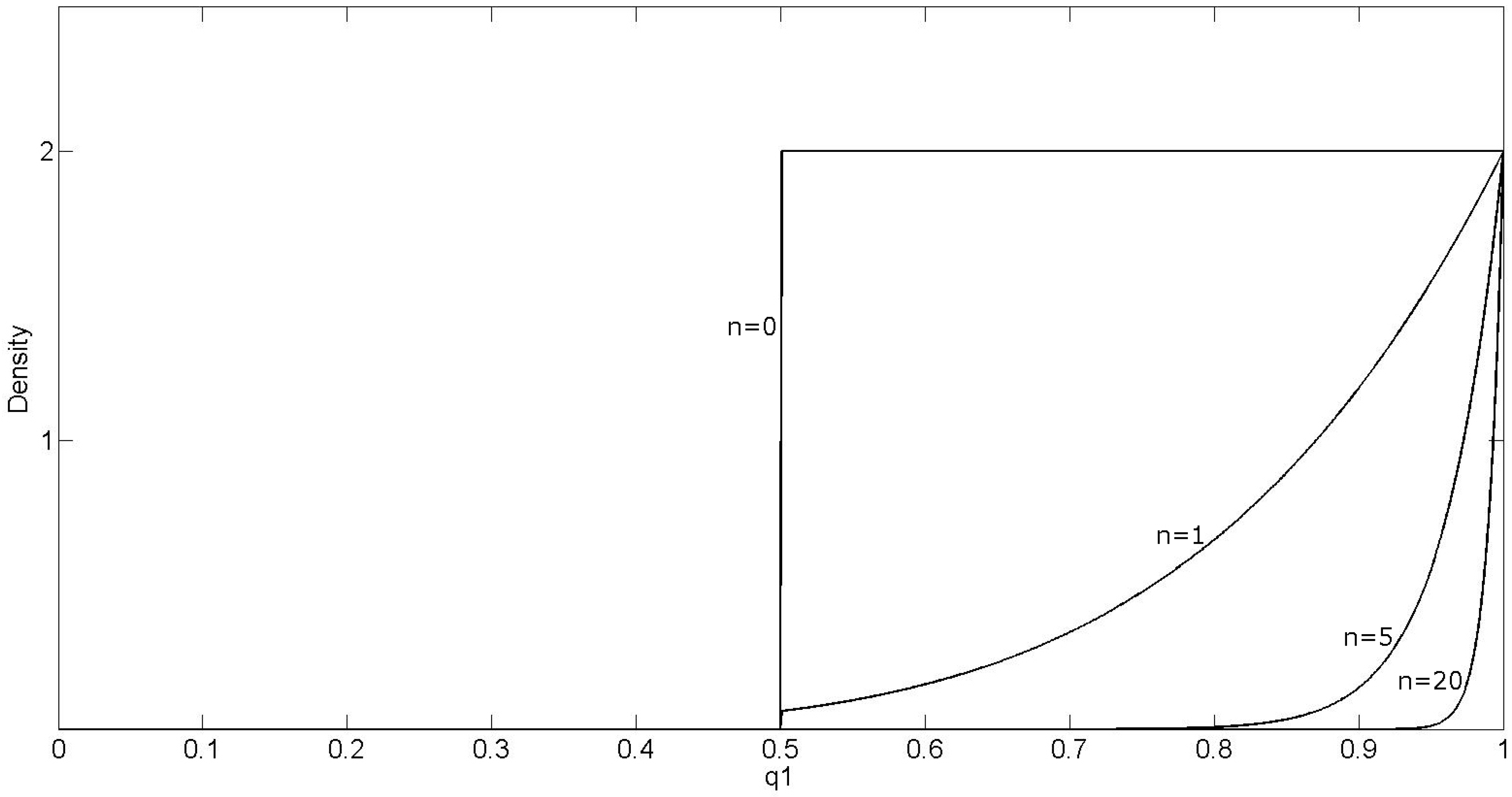
2.2. Accounting for Information about Volunteers’ Performance

Though the procedure presented in the previous section yields an estimate of $\mathbf{p}$ for a single volunteer when lacking information about its performance, it is of some concern to extend this approach for situations where this information exists, based on a validation dataset. Starting from a uniform distribution $f\left(\mathbf{q}\right)$, a standard Bayesian updating procedure allows us to additionally account for a given number of validation points.

In order to do so, let us consider in general the vector $\mathbf{n}=(n_0,...,n_k)$ where each $n_i$ is the number of validation points falling in the i-th category for a given contributor (with two categories here for our specific problem). We can thus compute the likelihood of observing this sample $\mathbf{n}$ from the corresponding multinomial distribution, where the probabilities of the various categories are given by $\mathbf{q}$, with:

$$P(\mathbf{N}=\mathbf{n}|\mathbf{q})=\frac{n!}{{\prod }_i{n}_i!}\prod _i{q}_i^{n_i}$$

(4)

where $n=n_0+\cdots +n_k$. A direct application of the Bayes theorem leads to the updated (i.e., the posterior distribution) $f(\mathbf{q}|\mathbf{N}=\mathbf{n})$, with:

$$f(\mathbf{q}|\mathbf{N}=\mathbf{n})\propto Likelihood\times Prior=P(\mathbf{N}=\mathbf{n}|\mathbf{q})\times f\left(\mathbf{q}\right)$$

(5)

As a conclusion, when facing a total lack of prior knowledge due to the lack of validation points, a natural choice based on the maximum entropy principle is to use the uniform $f\left(\mathbf{q}\right)$. More meaningful choices are however possible when validations points are at hand, so that an updated distribution $f(\mathbf{q}|\mathbf{N}=\mathbf{n})$ can be used instead. This flexibility is particularly interesting in a context where we need to handle at the same time volunteers with no performance assessment (i.e., using $f\left(\mathbf{q}\right)$) along with volunteers for which performance assessment is at hand through validation points (i.e., using $f(\mathbf{q}|\mathbf{N}=\mathbf{n})$). Clearly, this number of validation points may also vary from one volunteer to another one. Additionally, volunteers’ performance with respect to the same number of validation points may also widely vary from one volunteer to another one. All of these possibilities are handled through the use of Equation (5), so that a specific distribution can be used for each volunteer.

For an arbitrary number of categories and starting from a uniform prior $f\left(\mathbf{q}\right)$ over the simplex, the prior distribution $f\left(\mathbf{q}\right)$ corresponds to a Dirichlet distribution with a vector of parameters $\mathbf{\alpha }=({\mathbf{\alpha }}_0,\dots ,{\mathbf{\alpha }}_k)$, such that ${\alpha }_i=1$ $\forall i$, and the corresponding posterior distribution is also Dirichlet distributed over the same simplex. In our specific case where only two categories related to presence/absence are involved, the prior distribution for either $q_0$ or $q_1$ is uniform over $[0,1]$, and the corresponding posterior distribution is Betadistributed. This is illustrated in Figure 1, which shows how the shape of the (truncated) Beta posterior distribution is changing as the number of validation points is increasing. The fact that we start here from the uniform distribution over $[0.5,1]$ instead of $[0,1]$ is linked to the additional constraints $q_1>q_0$ to be fulfilled, so that values $q_1<0.5$ are impossible under this constraint.

2.3. Bayesian Data Fusion to Combine Multiple Volunteers’ Opinions at the Same Location

The Bayesian data fusion (BDF) methodology has been successively applied in various environmental contexts for combining multiple information sources relative to the same variable of interest, with the aim of increasing the final quality of the prediction. It has been widely studied for the prediction of continuous variables ([31,32,33]), and an extension was proposed in Gengler and Bogaert (2015) for categorical variables, as well.

Let us assume a categorical random variable Z where $z_0$ corresponds either to the presence/absence of cropland at the corresponding location ${\mathbf{x}}_0$, so that $z_0\in \{0,1\}$. Let us consider another set of categorical variables $E_{0,1},\dots ,E_{0,m}$ defined over the same set of categories and available at the prediction location ${\mathbf{x}}_0$, with observed values ${\mathbf{e}}_{\mathbf{0}}=(e_{0,1},\dots ,e_{0,m})$, where in our context, each $e_{0,i}$ corresponds to the cropland presence/absence as assigned by the i-th volunteer (i.e., $e_{0,i}\in \{0,1\}$ again). What we seek for are the conditional probabilities:

$$\begin{array}{ll}p(z_0|{\mathbf{e}}_{\mathbf{0}})& =\frac{p({\mathbf{e}}_{\mathbf{0}}|z_0)p\left(z_0\right)}{p\left({\mathbf{e}}_{\mathbf{0}}\right)}\\ & =\frac{p\left(z_0\right)}{p\left({\mathbf{e}}_{\mathbf{0}}\right)}{\displaystyle \prod _{i=1}^n}p(e_{0,i}|z_0)\\ & =\frac{p\left(z_0\right)}{p\left({\mathbf{e}}_{\mathbf{0}}\right)}{\displaystyle \prod _{i=1}^n}\frac{p(z_0|e_{0,i})p\left(e_{0,i}\right)}{p\left(z_0\right)}\\ & =\frac{1}{A}{p\left(z_0\right)}^{1-n}{\displaystyle \prod _{i=1}^n}p(z_0|e_{0,i})\end{array}$$

(6)

where the equality $p({\mathbf{e}}_{\mathbf{0}}|z_0)={\prod }_{i=1}^{n}p(e_{0,i}|z_0)$ corresponds to the mutual independence between the $E_i$’s conditionally to Z (see [26]) and where $A=p\left({\mathbf{e}}_{\mathbf{0}}\right)/{\prod }_{i}p\left(e_{i,0}\right)$ is a normalization constant ensuring that $\sum p(z_0|{\mathbf{e}}_{\mathbf{0}})=1$. Clearly, the probabilities $p(z_0|e_{0,i})$ (with $z_0\in \{0,1\}$, too) correspond to the previously described coding for each volunteer’s opinion about cropland presence/absence, i.e., the values for $p_0$ and $p_1$. The probabilities $p\left(z_0\right)$ are our prior information at that location before any volunteer opinion is made available. In this sense, Equation (6) allows us to update this prior information by accounting for the volunteers, and each ratio $p(z_0|e_{0,i})/p\left(z_0\right)$ is measuring the information content brought by the i-th volunteer with respect to the prior probability. Clearly, the more $p(z_0|e_{0,i})$ differs from $p\left(z_0\right)$, the more this volunteer will impact the final result. Finally, it is worth remembering again that the various $p{(z_0|e_{0,i})}^{\prime }s$ can be different, so that Equation (6) allows us to account at the same time for volunteers with varying performances.

2.4. Bayesian Maximum Entropy to Interpolate the Fused Volunteers Opinions

In order to get a map from the finite set of locations where crowdsourced information is at hand, it is needed to rely on a sound interpolation procedure. The Bayesian maximum entropy (BME) methodology allows us to do this from the fused volunteers’ opinions at various locations thanks to its ability to process the corresponding probabilistic (i.e., soft) information [34]. Indeed, we are here dealing with probability distributions $\widehat{\mathbf{p}}=(\widehat{P}(Z=1|\mathbf{e}),\widehat{P}(Z=0|\mathbf{e}))$, so that BME shows serious advantages compared to other classical interpolated methods as, e.g., the inverse distance weighted interpolation method that was used in [3]. In our case, the conditional probability distributions over the whole of Ethiopia are computed using the knowledge of the probability distributions at neighboring locations. The bivariate probabilities between the two classes as a function of the distance between the corresponding locations need to be estimated for this goal, and this was done according to the method advocated in [35].

2.5. Bayesian Data Fusion to Combine the Interpolated Map with the Land Cover

The BME methodology is providing us with a map solely based on the crowdsourced information, while on the other hand, we have a land cover product as derived from remote sensing. It is thus needed to get a single final map that would be based on these two information sources. This fusion of the BME interpolated map and the land cover product can be done using the BDF methodology again. Indeed, this corresponds to a particular case of the general BDF methodology, where no spatial structure needs to be taken into account and where the data sources are spatially exhaustive (i.e., the values are at hand for any arbitrary selected set of spatial locations). Xu et al. (2014) used a similar methodology for merging different land cover products, and their study can also be viewed as a particular case of the BDF equations [9].

Let us define $L_0$ as a categorical variable that corresponds to the cropland presence/absence as assigned by the land cover product at the prediction location, so that $l_0$ is its observed value. Similarly, let us consider $E_0^p$ as a categorical variable where $e_0^p$ corresponds to the cropland presence/absence at the prediction location as assigned by the interpolated map based on crowdsourced information. What we seek for is thus $p(z_0|e_0^p,l_0)$, i.e., the probability of presence/absence given the information provided both by the land cover product and the crowdsourced map. Using elementary probability properties, it thus comes that:

$$\begin{array}{ll}p(z_0|e_0^p,l_0)& =\frac{p(z_0,e_0^p,l_0)}{p(e_0^p,l_0)}\\ & =\frac{p\left(z_0\right)p(e_0^p,l_0|z_0)}{p(e_0^p,l_0)}\\ & =\frac{p\left(z_0\right)}{p(e_0^p,l_0)}p(e_0^p|z_0)p(l_0|z_0)\\ & =\frac{p\left(z_0\right)}{p(e_0^p,l_0)}\frac{p(z_0|e_0^p)p\left(e_0^p\right)}{p\left(z_0\right)}\frac{p(z_0|l_0)p\left(l_0\right)}{p\left(z_0\right)}\\ & =A\frac{p(z_0|e_0^p)p(z_0|l_0)}{p\left(z_0\right)}\end{array}$$

(7)

where the equality $p(e_0^p,l_0|z_0)=p(e_0^p|z_0)p(l_0|z_0)$ corresponds to the mutual independence between L and $E_0^p$ conditionally to Z and where $A=p\left(e_0^p\right)p\left(l_0\right)/p(e_0^p,l_0)$ is a normalization constant.

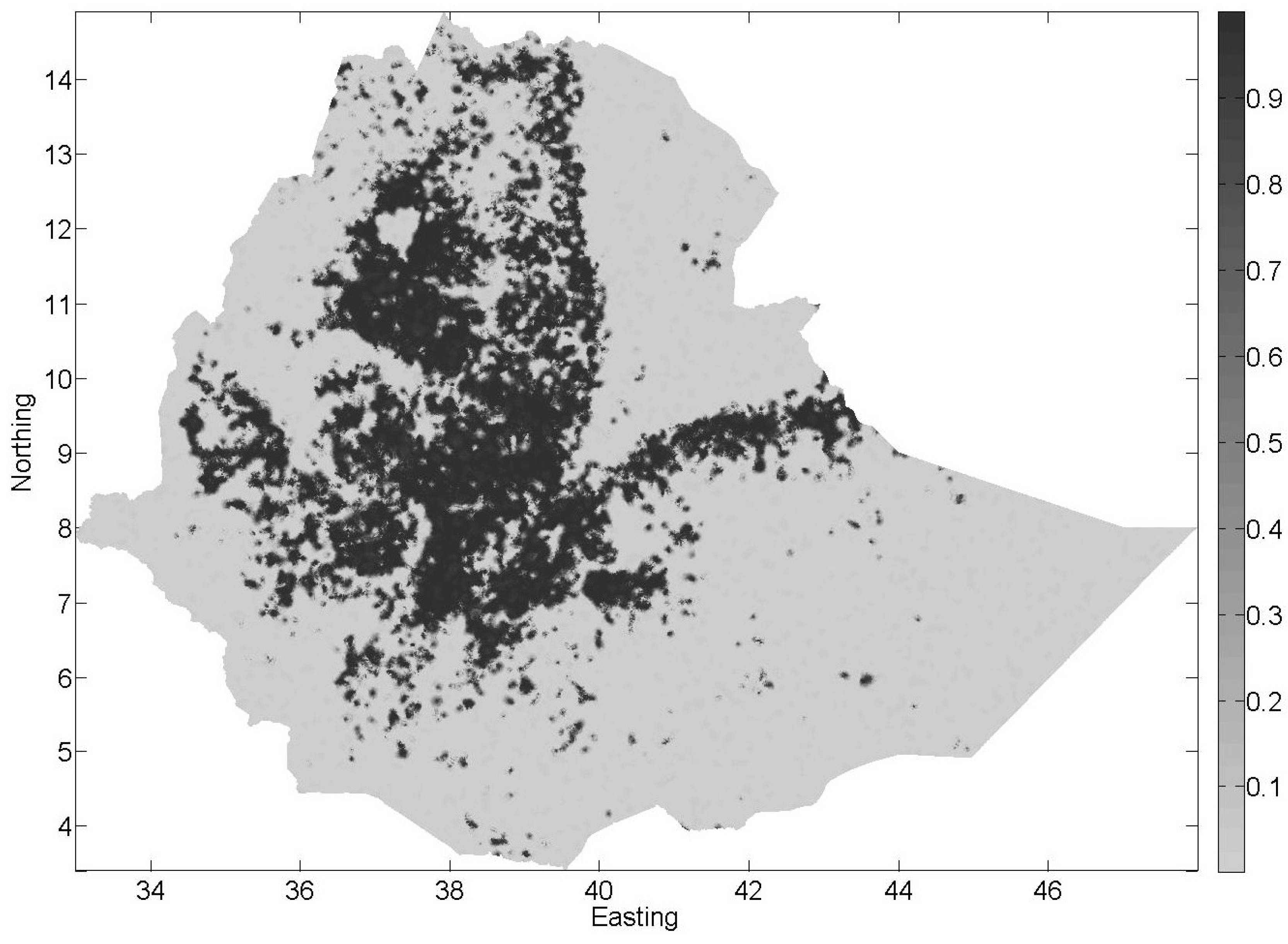
3. Results and Discussion

In order to illustrate the use of the proposed approach, we will focus on the spatial mapping of cropland in Ethiopia. For doing this, three sources of information were at hand, namely: (i) a land cover map as obtained in 2010 from the Climate Change Initiative land cover (CCI-LC) with a spatial resolution of 300 m [36]; (ii) an extensive crowdsourcing campaign that took place in 2012 and that involved data collection over the whole country; and (iii) a set of 1000 validation points as coming from an independent expert over the whole country, as well.

For the crowdsourcing campaign that was held in 2012, a Geo-wiki team asked volunteers to indicate the degree of cropland presence in samples of 1 km${}^2$ that were taken all over Ethiopia using Google Earth images. These data were collected using a simplified version of Geo-wiki [4]. A total of 32 volunteers indicated their opinion, and 77,465 contributions were collected. Three volunteers recorded more than 75% of these contributions (

Table 1. Volunteers’ contributions and validation points for the ten main contributors.

Contributor ID	Number of Contributions	Number of Validation Points
#1	20,497	279
#2	20,311	317
#3	19,238	284
#4	5575	83
#5	3311	49
#6	1536	29
#7	1534	16
#8	1427	11
#9	901	10
#10	659	10

). The classification was initially made using four classes of cropland occurrence, ranging from the absence of cropland to a high degree of cultivation [3]. For the present study, only two classes are defined by grouping the low, medium and high cultivation classes together. The variable of interest is thus a binary (i.e., Bernouilli) variable that corresponds to the absence/presence of cultivated land in Ethiopia (Figure 2). In parallel, from the Climate Change Initiative land cover product obtained in 2010, the same binary variable of interest was also derived. The label “presence of cultivated land” was associated with all land cover classes that contain cropland, i.e., rainfed, irrigated and post-flooding cropland and mosaic cropland. The remaining classes were labeled as “absence of cultivated land” (Figure 3). Finally, a validation dataset based on satellite data interpretation was built using a trained expert. A total of 1000 pixels randomly sampled over the whole of Ethiopia were investigated by this expert (Figure 4). This includes a subset of 500 locations where crowdsourced data were at hand. They are used to recode crowdsourced data (Section 3.1). Table 1 shows the number of validation points available for each of the 10 main contributors in the crowdsourcing exercise (these 10 main contributors representing 96.8% of the total crowdsourced data). The remaining 500 locations are not used in the calibration process. They are only used to assess the accuracy of the produced land cover maps (Section 3.5).

The CCI-LC product is far from being good for the specific cropland class, since this product is characterized by an overall accuracy of 76.8% (

Table 2. Confusion matrix for the CCI-LC product (for a total of 500 pixels).

		CCI-LC
		Crop	No Crop	Producer’s Accuracy (%)
Validation	Crop	110	14	88.71
	No crop	102	274	72.87
User’s Accuracy (%)		51.89	95.14	76.80

). Although the land cover has a fairly high user’s accuracy for the “no crop” class, this is not the case for the “crop” class. Indeed, if a pixel is labeled as “crop” by the land cover, the probability of actually observing a crop as measured by $P(Z=1|CCI=1)$ is only 51.9%. This means that no meaningful information can be obtained from the CCI-LC product when $CCI=1$ is occurring. As suggested in See et al. (2013), these errors could be explained by the similar spectral signatures exhibited by the cropland and grassland classes. In order to improve the land cover product, making use of crowdsourcing information is a possible alternative, especially in areas where the CCI-LC product is indicating the presence of crops.

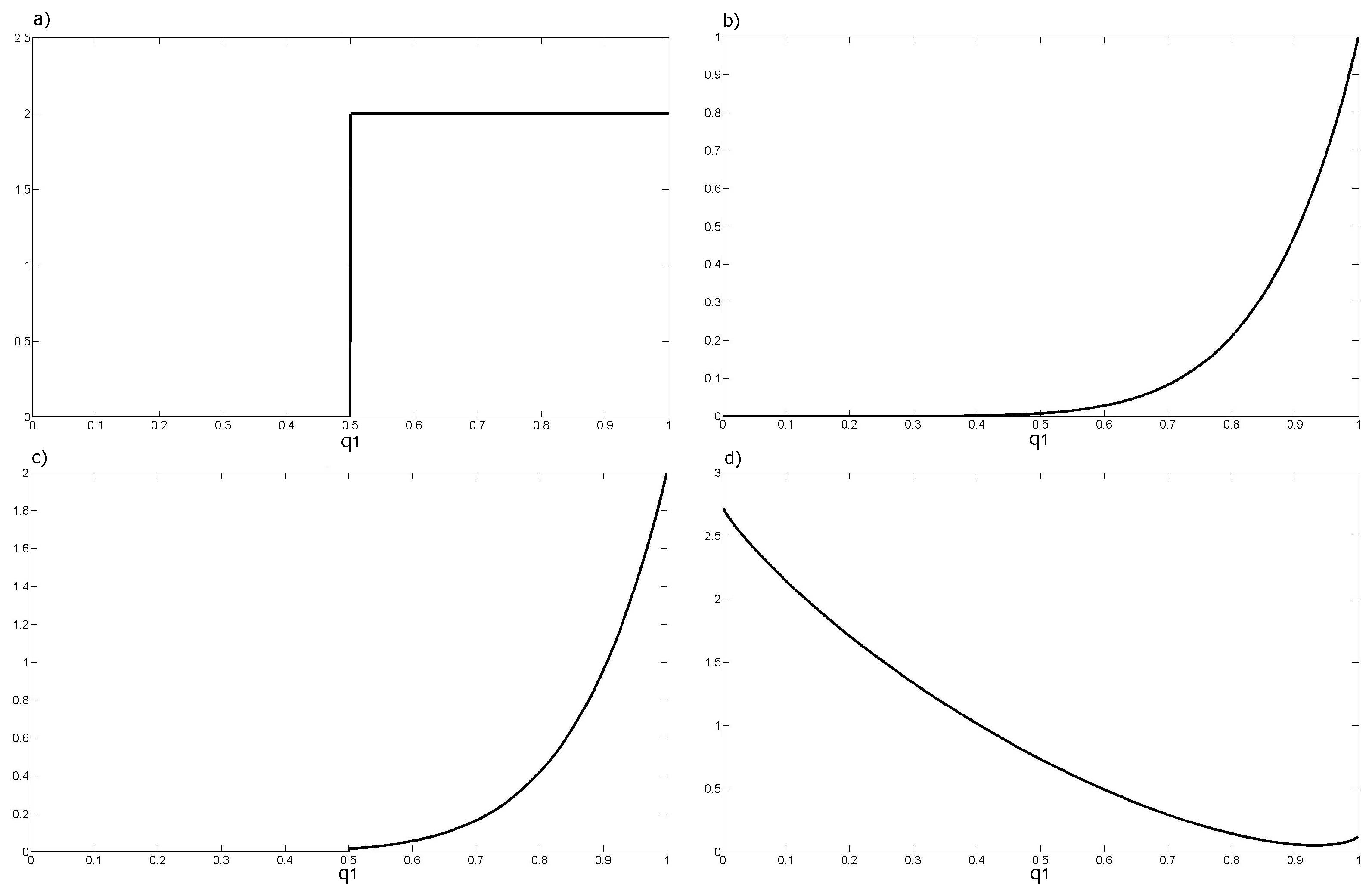
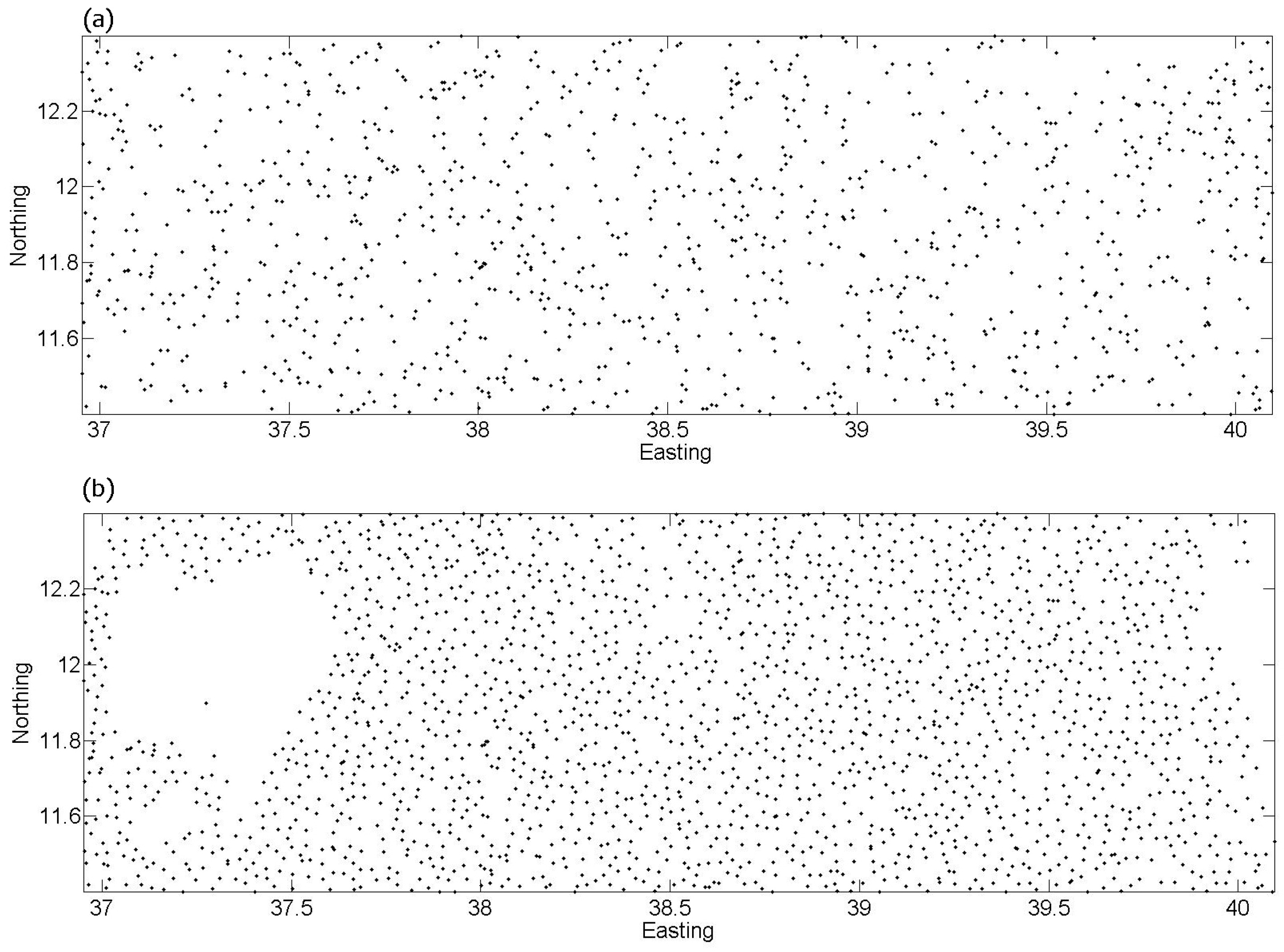
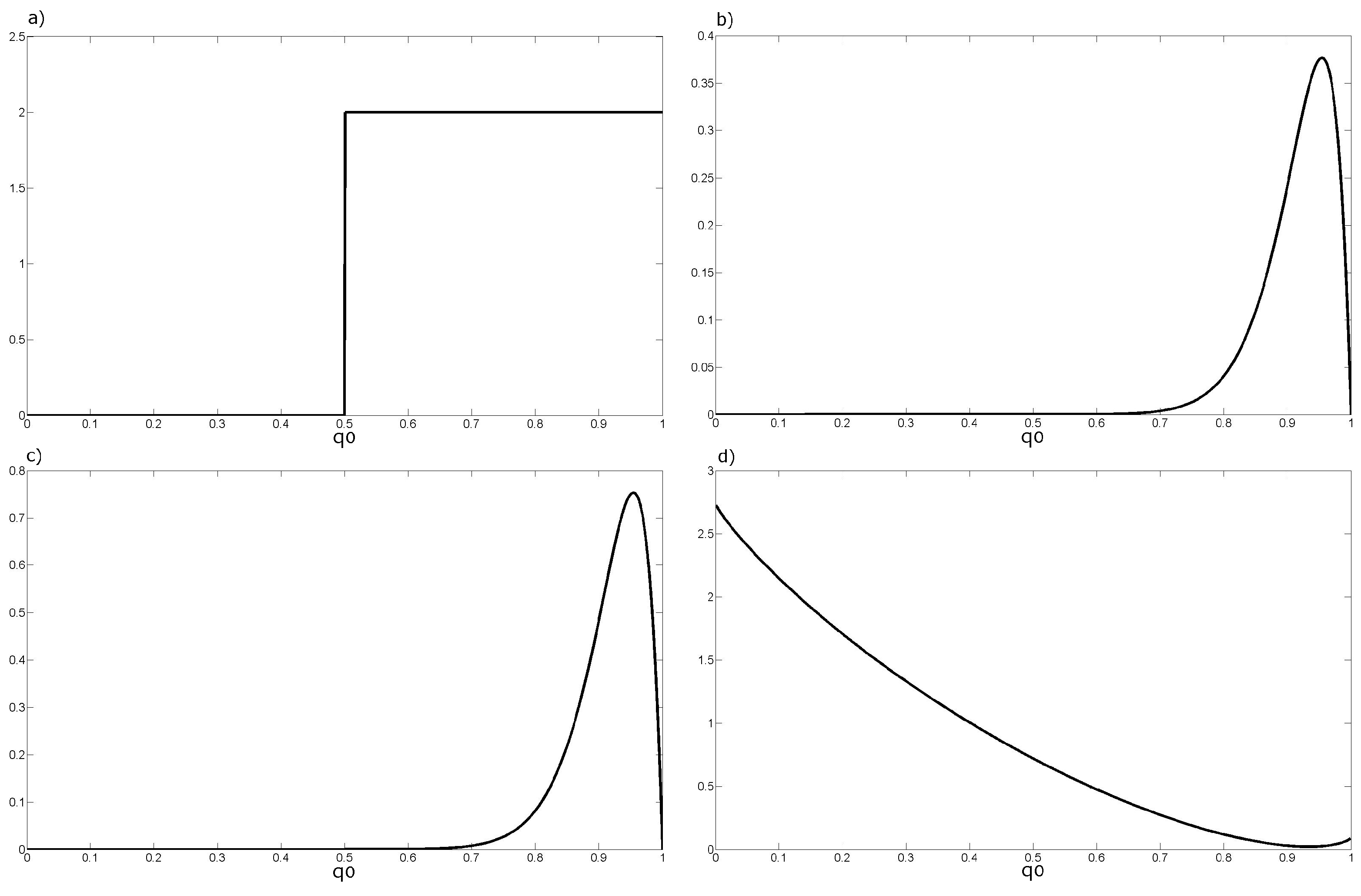
3.1. Recoding Crowdsourced Data

In order to combine crowdsourced information with this land cover product, contributors’ performances need to be estimated. The minimum divergence principle implemented by iterated MinNormapproximations is thus applied here to evaluate the quality of each contributor. When no information about a volunteer’s performance is at hand, a consistent choice is to use a uniform distribution $f\left(\mathbf{q}\right)$ over $S\cap C$, which leads to estimated values for the probabilities $p(z|e_i)$ (subject to the aforementioned inequality constraint) that are given by:

$$\begin{array}{cc}\widehat{P}(Z=1|E_i=1)=0.8\hfill & \widehat{P}(Z=0|E_i=1)=0.2\hfill \\ \\ \widehat{P}(Z=1|E_i=0)=0.2\hfill & \widehat{P}(Z=0|E_i=0)=0.8\hfill \end{array}$$

(8)

However, validation points are also at hand for 20 volunteers, so that more informative estimations for their performance can be obtained. In our specific problem, $\mathbf{n}=(n_0,n_1)$ where $n_1$ is the number of validation points that were assigned to the “crop” class, while $n_0$ are the assigned to the “no crop” class. The initial uniform distribution $f\left(\mathbf{q}\right)$ can then be modified accordingly using the classical Bayesian updating procedure (Figure 1), where the posterior distribution $f(\mathbf{q}|\mathbf{N}=\mathbf{n})$ may differ from one volunteer to another one depending on their respective performances.

As an illustration of the methodology and results, the case of Volunteer #6 is presented here in details For this volunteer, a total of 29 validation points are at hand, with seven points where this contributor is assigning the “crop” class (and so the “no crop” class was assigned for the 22 other validation points). In this particular case, $\mathbf{n}=(n_0=0,n_1=7)$ when Volunteer #6 is assigning the “crop” class and $\mathbf{n}=(n_0=21,n_1=1)$ when Volunteer #6 is assigning the “no crop” class. When this contributor is in favor of the presence of crop at a specific location ($E_6=1$), the constraint to be considered is thus $C=\{\mathbf{p}:p_1>p_0\}$. Let us start from the uniform distribution $f\left(\mathbf{q}\right)$, so that with $\mathbf{q}=(q_0,q_1)$, this reduces here to considering that:

$$f\left(\mathbf{q}\right)=\left\{\begin{array}{cc}2\hfill & \forall (q_0,q_1)\in S\cap C\hfill \\ \\ 0\hfill & \mathrm{otherwise}\hfill \end{array}\right.$$

(9)

where $S=\{\mathbf{p}:p_0\in [0,1],p_1\in [0,1],p_0+p_1=1\}$, where $n_0=0$ is the number of validation points attesting absence (the contributor is wrong at these locations), and $n_1=7$ is the number of validation points attesting presence (the contributor identifies correctly the true category at these locations). According to Equation (4), the likelihood of observing the sample $\mathbf{n}=(n_0=0,n_1=7)$ is thus given by:

$$P(\mathbf{N}=(0,7)|\mathbf{q})=\frac{7!}{(0!)(7!)}{\left(q_0\right)}^0{\left(q_1\right)}^7$$

(10)

From Equation (5), it is possible to update the prior $f\left(\mathbf{q}\right)$ based on the validation points available, leading to:

$$f(\mathbf{q}|\mathbf{N}=(0,7))\propto \left\{\begin{array}{cc}{\displaystyle \frac{7!}{(0!)(7!)}{\left(q_0\right)}^0{\left(q_1\right)}^7\times 2}\hfill & \forall (q_0,q_1)\in S\cap C\hfill \\ \hfill \\ 0otherwise.\hfill \end{array}\right.$$

(11)

Similarly, the same calculus can be done when the contributor is in favor of the absence of crop at a specific location (i.e., when $E_6=0$), so that the constraint now becomes $C=\{\mathbf{p}:p_0>p_1\}$. For the sake of illustration, Figure 5 and Figure 6 show: (a)the initial uniform prior when no information about the volunteer’s performance is taken into account; (b) the likelihood of observing a sample $\mathbf{n}$, i.e., $P(\mathbf{N}=(n_0,n_1)|q_1)$; (c) the corresponding updated distribution $f(q_1|\mathbf{n})$; and (d) the expected divergence $E\left[D\right(\mathbf{p}||\mathbf{Q}\left)\right]$ when Contributor #6 is in favor of the presence and the absence, respectively. As the same procedure can be applied for every volunteer,

Table 3. Minimum divergence approximations for the performances of the ten main contributors.

Contributor ID			E = 1	E = 0
#1	P(Z = 1 | E)		0.992	0.017
	P(Z = 0 | E)		0.008	0.983
#2	P(Z = 1 | E)		0.990	0.044
	P(Z = 0 | E)		0.010	0.956
#3	P(Z = 1 | E)		0.992	0.034
	P(Z = 0 | E)		0.008	0.966
#4	P(Z = 1 | E)		0.831	0.089
	P(Z = 0 | E)		0.169	0.911
#5	P(Z = 1 | E)		0.969	0.017
	P(Z = 0 | E)		0.031	0.983
#6	P(Z = 1 | E)		0.931	0.066
	P(Z = 0 | E)		0.069	0.934
#7	P(Z = 1 | E)		0.911	0.046
	P(Z = 0 | E)		0.089	0.954
#8	P(Z = 1 | E)		0.931	0.103
	P(Z = 0 | E)		0.069	0.897
#9	P(Z = 1 | E)		0.922	0.103
	P(Z = 0 | E)		0.078	0.897
#10	P(Z = 1 | E)		0.857	0.164
	P(Z = 0 | E)		0.143	0.836

summarizes the results for the ten main contributors by providing the values for $\widehat{\mathbf{p}}$ that correspond to the minimum value for the expected divergence $E\left[D\right(\mathbf{p}||\mathbf{Q}\left)\right]$.

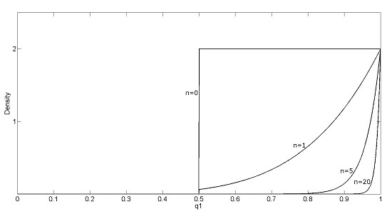
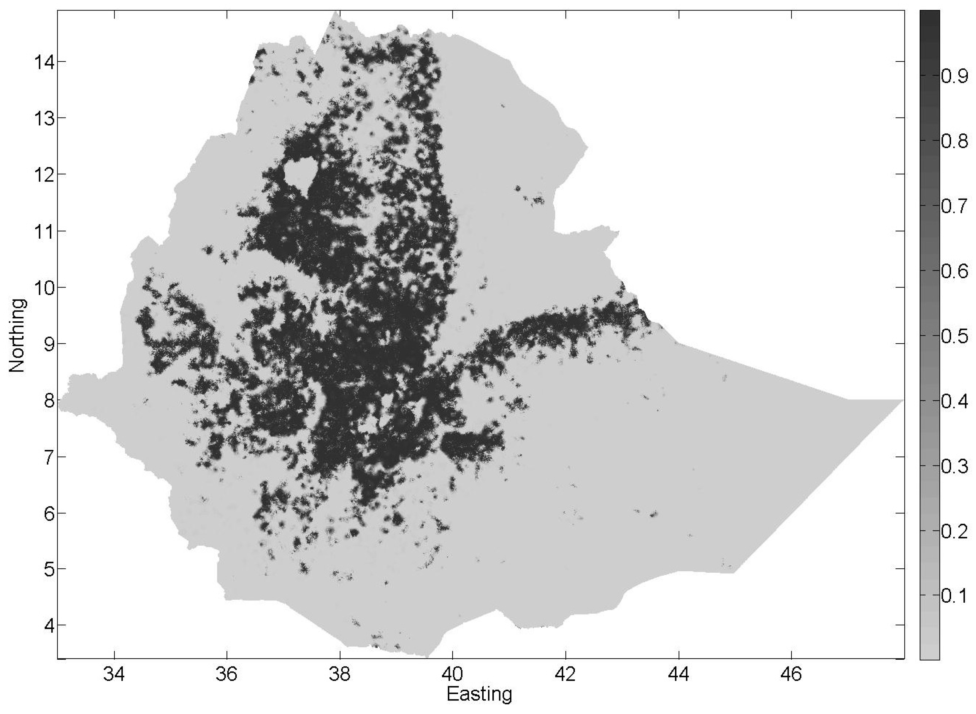
3.2. Fusion of Multiple Contributions at a Specific Location

During the crowdsourced exercise, volunteers investigated a total of 32,781 pixels, including 293 pixels that were labeled by a single volunteer only; while the vast majority of the pixels were inspected by at least two contributors. Therefore, multiple volunteers opinions can be combined at each location using the BDF methodology. For doing this, let us consider a specific pixel where a total of n volunteers whose performances are unknown give their opinion on the presence of cropland, so that there are $n_0$ volunteers assigning $E_i=0$, i.e., there are $n_1=n-n_0$ volunteers assigning $E_i=1$.

The prior distribution is assessed based on the validation set at hand, leading to $\widehat{P}(Z_0=0)=0.768$ and $\widehat{P}(Z_0=1)=0.232$. Accordingly, Equation (6) reduces now to:

$$\widehat{P}(Z=0|\mathbf{e})\propto 0.{768}^{1-n}{(0.8)}^{n_0}{(0.2)}^{n-n_0}$$

(12)

$$\widehat{P}(Z=1|\mathbf{e})\propto 0.{232}^{1-n}{(0.2)}^{n_0}{(0.8)}^{n-n_0}$$

(13)

If all volunteers agree with each other at a specific location, it is expected that the quality of the fused contributions increases with the number of volunteers [37]. This is the case with the BDF methodology, since the result will converge towards zero if $\widehat{P}(Z=1|E_i=1)<0.5$ $\forall i$, while it will converge towards one if $\widehat{P}(Z=1|E_i=1)>0.5$ $\forall i$.

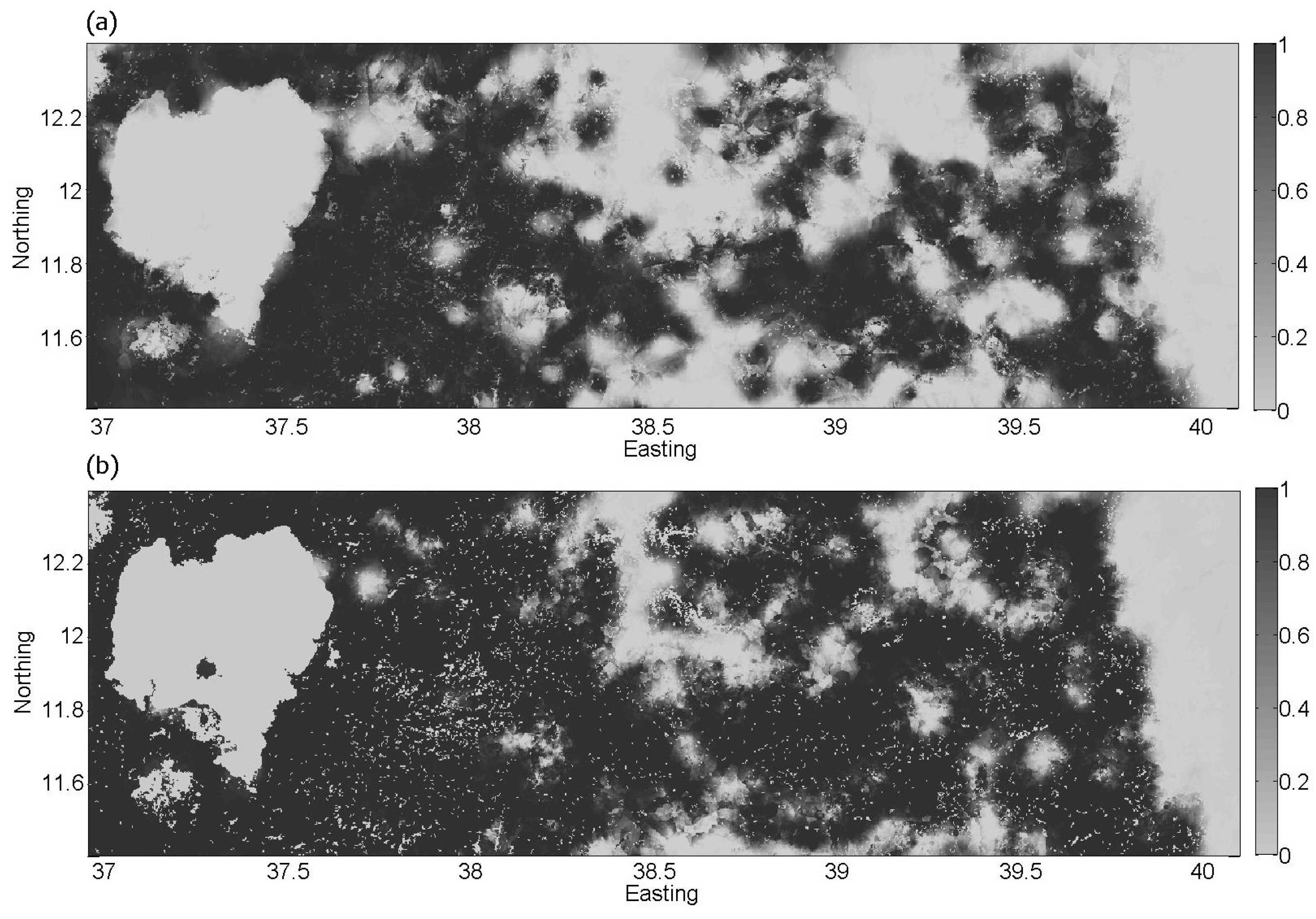
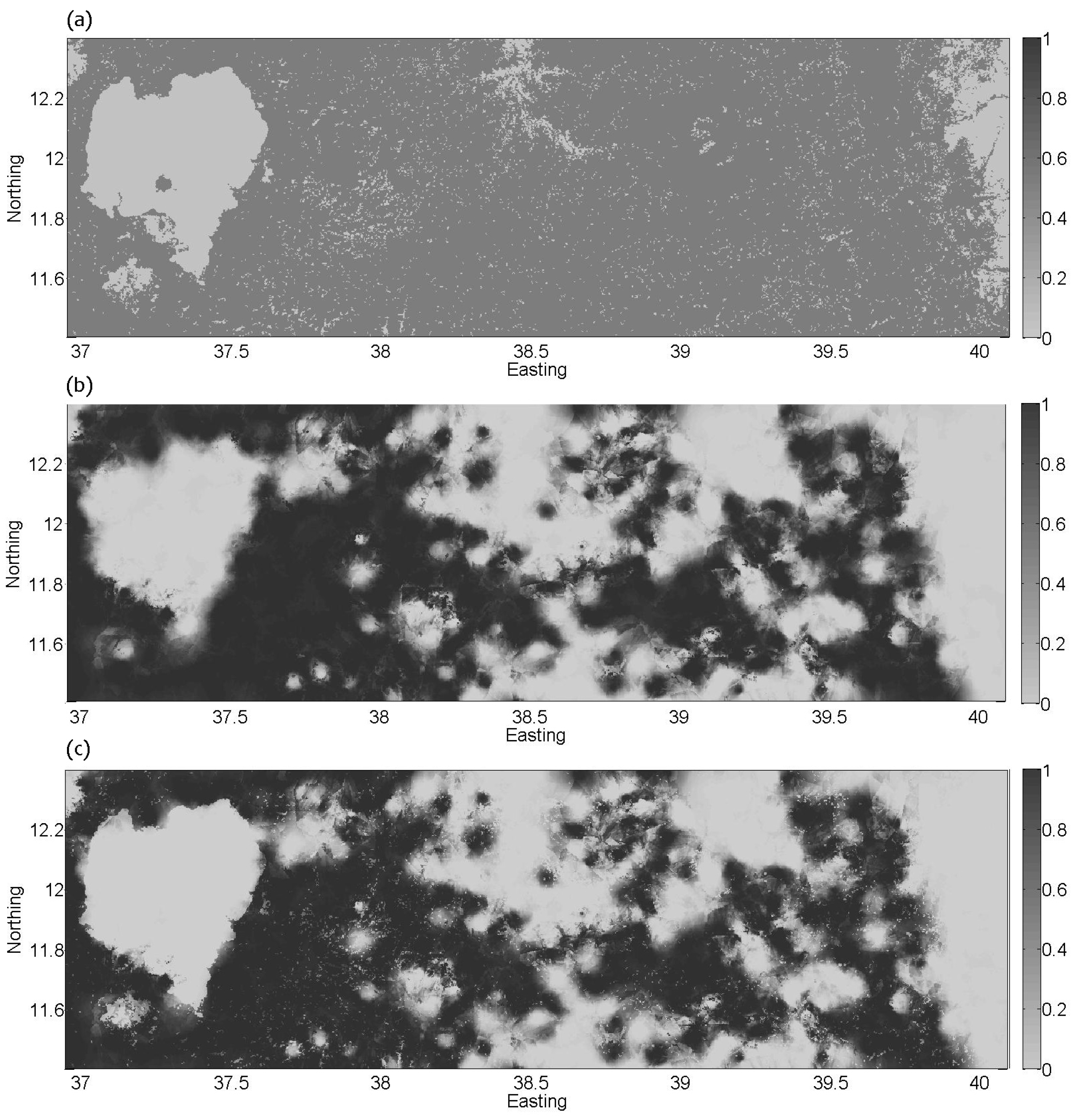
3.3. Fused Opinions Interpolation

Once multiple contributions are fused at each location, the Bayesian maximum entropy (BME) methodology for soft information is applied to interpolate the crowdsourced data over the whole of Ethiopia. Computations to estimate the spatial structure of the data are made on the basis of the 500 validation points where crowdsourced data are at hand along with the locations where the fused volunteers’ opinions that can virtually be considered as hard data, i.e., for locations where the probability $\widehat{P}(Z=0|\mathbf{e})>0.99$ or those where $\widehat{P}(Z=1|\mathbf{e})>0.99$. The interpolation is computed on the basis of the crowdsourced data only (no validation point is used at this step). The corresponding interpolated map is presented in Figure 7.

The quality of the interpolation depends on the spatial density of the crowdsourced information and on the spatial structure of the data. In our specific case, the quality of the interpolation is expected to be high, since crowdsourced data were sampled with a very high spatial density. However, in many cases, crowdsourced information is not available with such a high spatial density. In those cases, the interpolation may lead to poor results, and the fusion will only be possible locally, where crowdsourced data are available. When only a few crowdsourced data are available, they can be used locally to update the land cover product at a few locations where the crowdsourcing information is available, but they can also be an alternative source for collecting training samples and be used in combination with the satellite imagery itself to generate a land cover map [38,39].

3.4. Combining the Interpolated Map with the CCI-LC Product Using BDF

This interpolated map then needs to be combined with the CCI-LC product through the BDF methodology by relying on a conditional independence hypothesis, so that $p(e_0^p,l_0|z_0)=p(e_0^p|z_0)p(l_0|z_0)$. Stated otherwise, at the prediction location $x_0$, the categories derived from the CCI-LC product and the crowdsourcing data are independent from each other conditionally on the true category. As the results that one will obtain for the fused map rely on this conditional independence hypothesis, it is of some concern to test if it holds true. In order to test this assumption from the crowdsourced data at hand, a likelihood test of conditional independence has been used [40]. Generally speaking, let us consider that r, s and t are respectively the number of categories for the crowdsourced data, for the land cover product and for the validation set (with $r=s=t=2$ in our specific case). Let us consider i∈ [1, ⋯, r], j∈ [1, ⋯, s] and k∈ [1, ⋯, t]. Under the conditional independence null hypothesis ($H_0$), the conditional probabilities are given by:

$$\begin{array}{c}{H}_0\equiv p_{ij|k}=p_{i|k}{p}_{j|k}\hfill \\ \hfill \\ H_1\equiv \exists p_{ij|k}\ne p_{i|k}{p}_{j|k}\hfill \end{array}$$

$$\to A{H}_0\equiv G^2\le {\chi }_{1-\alpha }^2(r-1)(s-1)t$$

(14)

where the log-likelihood ratio $G^2$ is chi-squared distributed, with:

$$G^2=2\sum _{i,j,k}{N}_{ijk}ln\frac{N_{ijk}}{n{\widehat{p}}_{ijk}}\stackrel{n\to \infty }{\sim }{\chi }^2(r-1)(s-1)t$$

(15)

with $n=500$ here and where $N_{ijk}$ is the observed count of crowdsourced data where categories i, j and k are jointly observed. For our data, the conditional independence hypothesis is clearly acceptable, since $G^2=0.2511<{\chi }_{0.95}^2\left(2\right)=5.991$, corresponding to a p-value ($p_v$) equal to 0.8820. This result ensures that BDF is a suitable methodology to fuse the interpolated crowdsourced contributions and the land cover product in our context (see Figure 8).

Although there is no theoretical need for a very large crowdsourced dataset in order to use the method, it is however clear that the impact of the crowdsourced data on the update of the previous land cover product will be less significant if only a few crowdsourced data are at hand. The benefit of the method will of course be impacted by the amount of crowdsourced data. In our specific case, the benefit of the fusion is expected to be high, since crowdsourced data are sampled with a very high spatial density. However, in many cases, crowdsourced information is not sampled with such a high spatial density, and the benefit of the fusion will only appear locally, where few crowdsourced data are at hand.

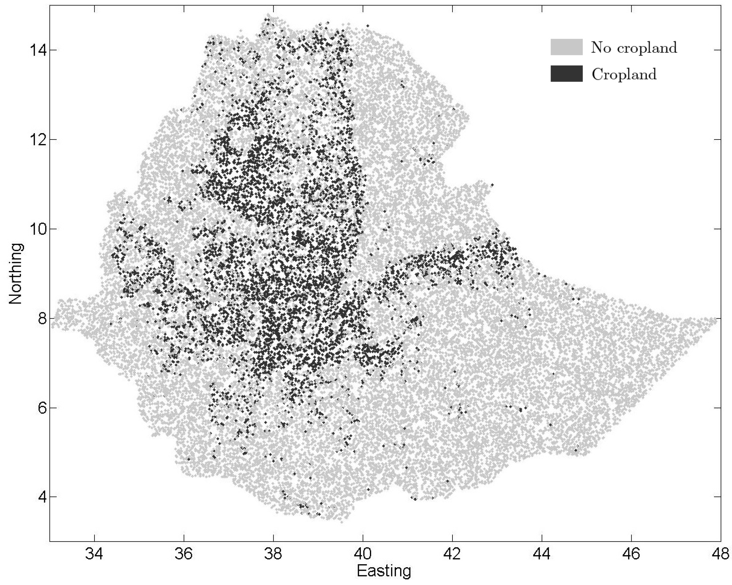
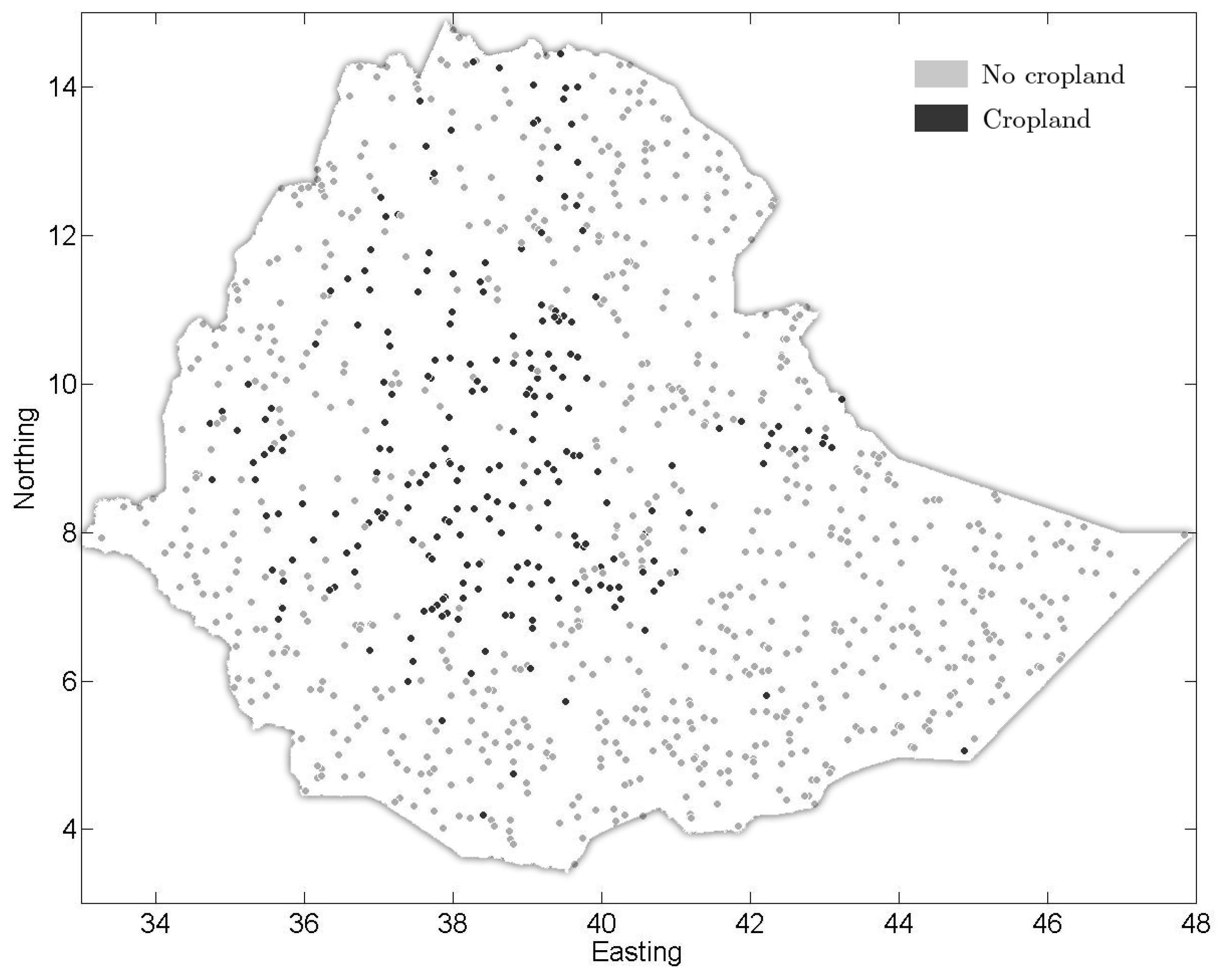
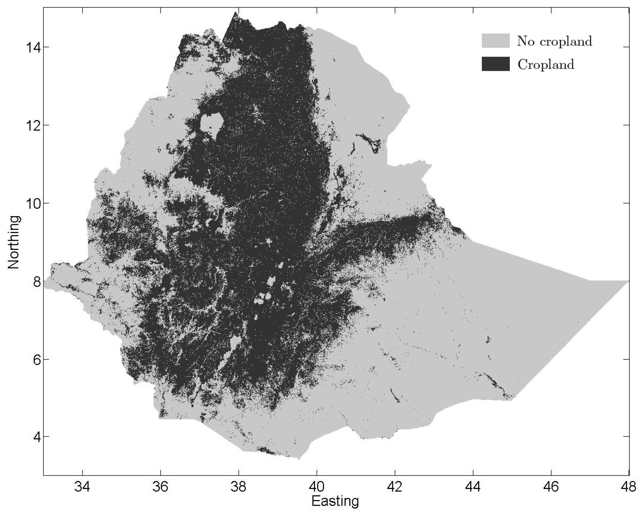
3.5. Comparison of the Three Land Cover Maps

In our specific case, three different products are thus compared for the cropland mapping over Ethiopia: the map derived from the land cover product only, the interpolated map based on the crowdsourced data only and the final fused map that combines the two previous ones. Table 2 indicates high errors of commission for the land cover product, since it assigns the “crop” label to many pixels where no cropland is found. It can be calculated that if the land cover product indicates the presence of crop, the probability of actually observing a crop is only 51.89% (P(Validation = 1|CCI = 1) = 0.52). However, the land cover product shows better results when assigning the “no crop” label, with $P(Validation=2|CCI=2)=0.95$. On the other side, the interpolated map based on the crowdsourced data performs better than the land cover product for correctly assigning the “crop” label with $P(Validation=1|crowdsourcing=1)=0.82$, and the “no crop” label is assigned with a similar performance than for the land cover product with $P(Validation=2|crowdsourcing=2)=0.92$.

In our specific case, it is expected that combining the crowdsourcing information with the land cover product might not lead to a significant improvement for the accuracy compared to the results obtained from the crowdsourced data alone. Indeed, the land cover product does not have a significant impact in the fused map in areas where the land cover assigns the label crop since it performs poorly compared to the crowdsourcing information. Moreover, the land cover product and the crowdsourced information generally agree with each other in areas where the land cover assigns the “no crop” label. For these very specific reasons that apply here, the fused map is expected to lead to results similar to those from the interpolated map based on the crowdsourced data.

In order to compare the quality of those three products, confusion matrices are computed for each of them (Table 2,

Table 4. Confusion matrix for the interpolated map based on crowdsourced data (for a total of 500 pixels).

		Interpolation Crowdsourcing
		Crop	No Crop	Producer’s Accuracy (%)
Validation	Crop	95	29	76.61
	No crop	21	355	94.41
User’s Accuracy (%)		81.90	92.45	98.00

and

Table 5. Confusion matrix for the cropland map based on the fusion of the CCI-LC product and the crowdsourced data (for a total of 500 pixels).

		Fusion CCI-LC-Crowdsourcing
		Crop	No Crop	Producer’s Accuracy (%)
Validation	Crop	94	30	75.81
	No crop	20	356	94.68
User’s Accuracy (%)		82.46	92.23	98.00

). For the two maps produced with crowdsourcing information, these matrices do not indicate significant differences according to a chi-square test based on the comparison of two multinomial distributions with related samples (${\chi }_{obs}^2=0.667$, p-value = 0.4142). These maps show a higher overall accuracy (98%) compared to the map based on the land cover product only (76.8%). A McNemar’s test [41] confirms that this difference is highly significant ($p_v\simeq {10}^{-10}$).

In order to ease the visual comparison and to illustrate the results, a smaller area around Lake Tana is considered for comparing the three cropland maps (Figure 9). Both maps including crowdsourced data show very similar patterns, with differences that appear in areas where the land cover map assigns the “no crop” label, opposite of the map based on crowdsourced data only. It can be seen that that, for the fused map, the limits of Lake Tana are better defined than they are for the crowdsourced map.

During the crowdsourced exercise held in 2012, the 77,465 pixels that were investigated by volunteers were randomly selected over the whole country [3]. However, since the land cover product performs well when it assigns the “no crop” label, the crowdsourcing campaign could have been optimized by focusing on areas where the land cover product is known to perform badly (i.e., areas where it assigns the “crop” label). In the CCI-LC product, 40.8% of the pixels are labeled as cropland. As there is little expected benefit of investigating the other pixels, the sampling could have been restricted to these pixels only, increasing in this way the amount of useful crowdsourced information for the same sampling effort.

During the 2012 campaign around Lake Tana, out of the total number of 2091 pixels that were investigated by volunteers, only 857 pixels were labeled as “crop” by the CCI-LC product. If all of the sampling effort had been concentrated on these “crop” labeled pixels, the quality of the product could have been significantly improved at no extra cost. To illustrate the potential benefits of an optimized crowdsourcing campaign, two volunteers were asked to investigate 2091 − 857 = 1234 additional pixels among those “no crop” labeled pixels (Figure 10). The map resulting from the fusion that now accounts for these 1234 extra crowdsourced pieces of information illustrates the corresponding improvement (Figure 11).

4. Conclusions

An accurate spatial mapping of cropland is compulsory for many applications, but cropland maps solely based on land cover products as obtained from satellite data are far from being perfect. In this paper, it is suggested that integrating crowdsourced data with land cover products might improve the accuracy of the final cropland map. However, assessing the quality of a volunteer’s contribution in a crowdsourcing exercise might be difficult in many cases.

In this paper, it is shown how contributors’ performances can be assessed through the minimum divergence and the maximum entropy principles. The information brought by contributors is first coded in terms of inequality constraints, and performance estimation is computed afterwards. Results shown in this paper suggest that it is worthwhile to include crowdsourced data in the spatial prediction of cropland, even if no prior information about the contributors performances is at hand. The map obtained from the fusion of the CCI-LC product with crowdsourced information shows a better overall accuracy compared to the cropland map based on the CCI-LC dataset only. However, for the specific case of cropland mapping over Ethiopia that was presented here, the fused map is close to the cropland map based on the crowdsourced data only. Differences appear only in a few areas where the land cover product disagrees with the crowdsourced map by assigning the “no crop” label. This is a direct consequence of the fact that the CCI-LC product performs poorly when assigning the “crop” label, while the performances of the crowdsourced information is close to the CCI-LC product when the “no crop” label is assigned.

Clearly, the low benefit of the fused map over the cropland map based on crowdsourced data only can be viewed as a consequence of the fact that both source of information were collected in a totally independent way. Indeed, the crowdsourcing campaign was held regardless of the land cover product results, though a prior assessment could have been done prior to the crowdsourcing, so that the crowdsourcing campaign could have been easily optimized at no extra cost by focusing on areas where the CCI-LC product is known to be deficient (i.e., when it assigns the “crop” label). A sound prior assessment of remotely-sensed data quality can thus seriously improve the benefit of subsequent crowdsourcing campaigns and the benefit of fusing information afterwards, by maximizing the benefit of using each source of information. Based on this single application of cropland mapping in Ethiopia, we believe that our paper also emphasizes the high potential of crowdsourced data for improving land cover products. With this goal in mind, the BDF methodology and the corresponding processing framework that was proposed appear to offer a promising alternative compared to more traditional approaches.

References

1. Fritz, S.; McCallum, I.; Schill, C.; Perger, C.; Grillmayer, R.; Achard, F.; Kraxner, F.; Obersteiner, M. Geo-Wiki.Org: The use of crowdsourcing to improve global land cover. Remote Sens. 2009, 1, 345–354. [Google Scholar] [CrossRef]
2. Fritz, S.; You, L.; Bun, A.; See, L.; McCallum, I.; Schill, C.; Perger, C.; Liu, J.; Hansen, M.; Obersteiner, M. Cropland for sub-Saharan Africa: A synergistic approach using five land cover data sets. Geophys. Res. Lett. 2011, 38. [Google Scholar] [CrossRef]
3. See, L.; McCallum, I.; Fritz, S.; Perger, C.; Kraxner, F.; Obersteiner, M.; Baruah, U.D.; Mili, N.; Kalita, N.R. Mapping cropland in Ethiopia using crowdsourcing. Int. J. Geosci. 2013, 4, 6–13. [Google Scholar] [CrossRef]
4. See, L.; Fritz, S.; You, L.; Ramankutty, N.; Herrero, M.; Justice, C.; Becker-Reshef, I.; Thornton, P.; Erb, K.; Gong, P.; et al. Improved global cropland data as an essential ingredient for food security. Glob. Food Secur. 2015, 4, 37–45. [Google Scholar] [CrossRef] [Green Version]
5. Hansen, M.C.; DeFries, R.S.; Townshend, J.R.G. Global land cover classification at 1 km spatial resolution using a classification tree approach. Int. J. Remote Sens. 2000, 21, 1331–1364. [Google Scholar] [CrossRef]
6. Jung, M.; Henkel, K.; Herold, M.; Churkina, G. Exploiting synergies of global land cover products for carbon cycle modeling. Remote Sens. Environ. 2006, 101, 534–553. [Google Scholar]
7. Pérez-Hoyos, A.; García-Haro, F.; San-Miguel-Ayanz, J. A methodology to generate a synergetic land-cover map by fusion of different land-cover products. Int. J. Appl. Earth Observ. Geoinf. 2012, 19, 72–87. [Google Scholar]
8. See, L.; Fritz, S. A method to compare and improve land cover datasets: Application to the GLC-2000 and MODIS land cover products. IEEE Trans. Geosci. Remote Sens. 2006, 44, 1740–1746. [Google Scholar] [CrossRef]
9. Xu, G.; Zhang, H.; Chen, B.; Zhang, H.; Yan, J.; Chen, J.; Che, M.; Lin, X.; Dou, X. A bayesian based method to generate a synergetic land-cover map from existing land-cover products. Remote Sens. 2014, 6, 5589–5613. [Google Scholar] [CrossRef]
10. Cardille, J.A. Characterizing Patterns of Agricultural Land Use in Amazonia By Merging Satellite Imagery and Census Data. Ph.D. Thesis, University of Wisconsin-Madison, Madiso, WM, USA, 2002. [Google Scholar]
11. Cardille, J.A.; Clayton, M.K. A regression tree-based method for integrating land-cover and land-use data collected at multiple scales. Environ. Ecol. Stat. 2007, 14, 161–179. [Google Scholar] [CrossRef]
12. Hurtt, G.C.; Rosentrater, L.; Frolking, S.; Moore, B. Linking remote-sensing estimates of land cover and census statistics on land use to produce maps of land use of the conterminous United states. Glob. Biogeochem. Cycl. 2001, 15, 673–685. [Google Scholar] [CrossRef]
13. Fonte, C.C.; Bastin, L.; See, L.; Foody, G.; Lupia, F. Usability of VGI for validation of land cover maps. Int. J. Geogr. Inf. Sci. 2015, 29, 1269–1291. [Google Scholar] [CrossRef]
14. Muller, C.; Chapman, L.; Johnston, S.; Kidd, C.; Illingworth, S.; Foody, G.; Overeem, A.; Leigh, R. Crowdsourcing for climate and atmospheric sciences: Current status and future potential. Int. J. Climatol. 2015, 35, 3185–3203. [Google Scholar] [CrossRef]
15. Poser, K.; Dransch, D. Volunteered Geographic Information for Disaster Management with Application to Rapid Flood Damage Estimation. Geomatica 2010, 64, 89–98. [Google Scholar]
16. Roche, S.; Propeck-Zimmermann, E.; Mericskay, B. GeoWeb and crisis management: issues and perspectives of volunteered geographic information. GeoJournal 2011, 78, 21–40. [Google Scholar] [CrossRef]
17. Zook, M.; Graham, M.; Shelton, T.; Gorman, S. Volunteered geographic information and crowdsourcing disaster relief: A case study of the Haitian Earthquake. World Med. Health Policy 2010, 2, 6–32. [Google Scholar] [CrossRef]
18. Coleman, D.J.; Sabone, B.; Nkhwanana, N. Volunteering geographic information to authoritative databases: Linking contributor motivations to program effectiveness. Geomatica 2013, 64, 383–396. [Google Scholar]
19. Sui, D.; Elwood, S.; Goodchild, M. Crowdsourcing Geographic Knowledge; Springer: Berlin, Germany, 2013. [Google Scholar]
20. Goodchild, M.F.; Glennon, J.A. Crowdsourcing geographic information for disaster response: A research frontier. Int. J. Digit. Earth 2010, 3, 231–241. [Google Scholar] [CrossRef]
21. Goodchild, M.F.; Li, L. Assuring the quality of volunteered geographic information. Spatial Stat. 2012, 1, 110–120. [Google Scholar] [CrossRef]
22. Hunter, J.; Alabri, A.; Ingen, C.V. Assessing the quality and trustworthiness of citizen science data. Concurr. Comput. Pract. Exp. 2013, 25, 454–466. [Google Scholar] [CrossRef]
23. Comber, A.; See, L.; Fritz, S.; Van der Velde, M.; Perger, C.; Foody, G. Using control data to determine the reliability of volunteered geographic information about land cover. Int. J. Appl. Earth Observ. Geoinf. 2013, 23, 37–48. [Google Scholar] [CrossRef]
24. Bogaert, P.; Gengler, S. MinNorm approximation of MaxEnt/MinDiv problems for probability tables. In Proceedings of the Bayesian Inference and Maximum Entropy Methods in Science and Engineering MaxEnt 2014, Amboise, France, 21–26 September 2014; pp. 287–296.
25. Gengler, S.; Bogaert, P. Bayesian data fusion for spatial prediction of categorical variables in environmental sciences. In Proceedings of the Bayesian Inference and Maximum Entropy Methods in Science and Engineering MaxEnt 2013, Canberra, Australia, 15–20 September 2013; pp. 88–93.
26. Gengler, S.; Bogaert, P. Bayesian data fusion applied to soil drainage classes spatial mapping. Math. Geosci. 2015, 48, 79–88. [Google Scholar] [CrossRef]
27. Negash, M.; Swinnen, J.F. Biofuels and food security: Micro-evidence from Ethiopia. Energy Policy 2013, 61, 963–976. [Google Scholar] [CrossRef]
28. Waldner, F.; Fritz, S.; Di Gregorio, A.; Defourny, P. Mapping priorities to focus cropland mapping activities: Fitness assessment of existing global, regional and national cropland maps. Remote Sens. 2015, 7, 7959–7986. [Google Scholar] [CrossRef] [Green Version]
29. Tang, W.; Lease, M. Semi-supervised consensus labeling for crowdsourcing. In Proceedings of the SIGIR 2011 Workshop on Crowdsourcing for Information Retrieval, Beijing, China, 28 July 2011; pp. 36–41.
30. Wahyudi, A.; Bartzke, M.; Küster, E.; Bogaert, P. Maximum entropy estimation of a Benzene contaminated plume using ecotoxicological assays. Environ. Pollut. 2013, 172, 170–179. [Google Scholar] [CrossRef] [PubMed]
31. Bogaert, P.; Fasbender, D. Bayesian data fusion in a spatial prediction context: A general formulation. Stoch. Environ. Res. Risk Assess. 2007, 21, 695–709. [Google Scholar] [CrossRef]
32. Fasbender, D.; Peeters, L.; Bogaert, P.; Dassargues, A. Bayesian data fusion applied to water table spatial mapping. Water Resour. Res. 2008, 44, w12422. [Google Scholar] [CrossRef]
33. Fasbender, D.; Radoux, J.; Bogaert, P. Bayesian data fusion for adaptable image pansharpening. IEEE Trans. Geosci. 2008, 46, 1847–1857. [Google Scholar] [CrossRef]
34. D’Or, D.; Bogaert, P. Continous-valued map reconstruction with the Bayesian Maximum Entropy. Geoderma 2003, 112, 169–178. [Google Scholar] [CrossRef]
35. D’Or, D.; Bogaert, P. Combining categorical information with the Bayesian Maximum Entropy approach. In geoENV IV—Geostatistics for Environmental Applications; Springer: Dordrecht, The Netherlands, 2004. [Google Scholar]
36. Defourny, P.; Kirches, G.; Brockmann, C.; Boettcher, M.; Peters, M.; Bontemps, S.; Lamarche, C.; Schlerf, M.; Santoro, M. Land Cover CCI : Product User Guide Version 2. Available online: http://maps.elie.ucl.ac.be/CCI/viewer/download/ESACCI-LC-PUG-v2.5.pdf (accessed on 28 January 2016).
37. Haklay, M.; Basiouka, S.; Antoniou, V.; Ather, A. How many volunteers does it take to map an area well? The validity of Linus’ Law to volunteered geographic information. Cartogr. J. 2010, 47, 315–322. [Google Scholar] [CrossRef]
38. Arsanjani, J.J.; Helbich, M.; Bakillah, M. Exploiting volunteered geographic information to ease land use mapping of an urban landscape. Int. Arch. Photogram. Remote Sens. Spatial Inf. Sci. 2013, 1, 51–55. [Google Scholar] [CrossRef]
39. Johnson, B.A.; Iizuka, K. Integrating OpenStreetMap crowdsourced data and Landsat time-series imagery for rapid land use/land cover (LULC) mapping: Case study of the laguna Bay area of the Philippines. Appl. Geogr. 2016, 67, 140–149. [Google Scholar] [CrossRef]
40. Sokal, R.R.; Rohlf, F.J. Biometry; Freeman and Company: San Francisco, CA, USA, 1969. [Google Scholar]
41. Foody, G.M. Thematic map comparison: Evaluating the statistical significance of differences in classification accuracy. Photogram. Eng. Remote Sens. 2004, 7, 627–633. [Google Scholar] [CrossRef]
Figure 1. Modification of f ( q 1 ) as the number n of validation points increases for a volunteer who always identifies correctly the true category (i.e., n 1 = n and n 0 = 0 , with n 0 + n 1 = n ).
Remotesensing 08 00545 g001
Figure 2. Locations for the crowdsourced information; light grey dots correspond to the “no cropland” class, while black dots correspond to the “cropland” class (for a total of 32,781 pixels with an average density of 0.03 pixels/km 2 ).
Remotesensing 08 00545 g002
Figure 3. Cropland map based on the Climate Change Initiative land cover (CCI-LC) product for the year 2010; light grey dots correspond to the “no cropland” class, while black dots correspond to the “cropland” class.
Remotesensing 08 00545 g003
Figure 4. Locations for the 1000 validation points; light grey dots correspond to the “no cropland” class, while black dots correspond to the “cropland” class.
Remotesensing 08 00545 g004
Figure 5. (a) Initial uniform prior when no information about the volunteer’s performance is taken into account; (b) likelihood of observing a sample n , i.e., P ( N = ( n 0 , n 1 ) | q 1 ) ; (c) the corresponding updated distribution f ( q 1 | n ) ; and (d) the expected divergence E [ D ( p | | Q ) ] for the case where E 6 = 1 .
Remotesensing 08 00545 g005
Figure 6. (a) Initial uniform prior when no information about the volunteer’s performance is taken into account; (b) likelihood of observing a sample n , i.e., P ( N = ( n 0 , n 1 ) | q 0 ) ; (c) the corresponding updated distribution f ( q 0 | n ) ; and (d) the expected divergence E [ D ( p | | Q ) ] for the case where E 6 = 0 .
Remotesensing 08 00545 g006
Figure 7. Cropland map based on the crowdsourced data showing the probability of observing the “crop” class over Ethiopia.
Remotesensing 08 00545 g007
Figure 8. Cropland map based on the fusion of the crowdsourced data with the land cover product showing the probability of observing the “crop” class over Ethiopia.
Remotesensing 08 00545 g008
Figure 9. Cropland maps around Lake Tana showing the probability of observing the “crop” class based on (a) the CCI-LC product; (b) the interpolated map based on the volunteers’ opinions and (c) the fusion of the CCI-LC product and volunteers’ opinions.
Remotesensing 08 00545 g009
Figure 10. Sampled pixels around Lake Tana (a) for the crowdsourced exercise held in 2012 and (b) when the sampling is optimized based on the performance of the CCI-LC product.
Remotesensing 08 00545 g010
Figure 11. Cropland maps around Lake Tana showing the probability of observing the “crop” class based on (a) the fusion of the CCI-LC product and volunteers’ opinions and (b) the fusion of the CCI-LC product and volunteers’ opinions when the sampling is optimized based on the performance of the CCI-LC product.
Remotesensing 08 00545 g011