Article

Mangroves at Their Limits: Detection and Area Estimation of Mangroves along the Sahara Desert Coast

by
Viviana Otero
1,*,
Katrien Quisthoudt
1,
Nico Koedam
2,† and
Farid Dahdouh-Guebas
1,2,†
1
Laboratory of Systems Ecology and Resource Management, Faculté des Sciences, Université Libre de Bruxelles (ULB), Avenue F.D. Roosevelt 50, CPI 264/1, B-1050 Brussels, Belgium
2
Laboratory of Plant Biology and Nature Management, Ecology and Biodiversity, Faculty of Science and Bio-Engineering Sciences, Vrije Universiteit Brussel (VUB), Pleinlaan 2, VUB-APNA-WE, B-1050 Brussels, Belgium
*
Author to whom correspondence should be addressed.
These authors contributed equally to this work.
Remote Sens. 2016, 8(6), 512; https://doi.org/10.3390/rs8060512
Submission received: 31 March 2016 / Revised: 27 May 2016 / Accepted: 14 June 2016 / Published: 18 June 2016
(This article belongs to the Special Issue Remote Sensing in Coastal Environments)

Abstract

:
The northernmost and most arid mangrove ecosystem of West Africa is found in Mauritania, in the Parc National du Banc d’Arguin (PNBA). The existing global and regional maps of Mauritania’s mangroves have little detail, and available estimates of the mangrove area differ among studies. We assessed the use of automated Remote Sensing classification techniques to calculate the extent and map the distribution of the mangrove patches located at Cap Timiris, PNBA, using QuickBird and GeoEye imagery. It was possible to detect the northernmost contiguous mangrove patches of West Africa with an accuracy of 87% ± 2% using the Maximum Likelihood algorithm. The main source of error was the low spectral difference between mangroves and other types of terrestrial vegetation, which resulted in an erroneous classification between these two types of land cover. The most reliable estimate for the mangrove area obtained in this study was 19.48 ± 5.54 ha in 2011. Moreover, we present a special validation procedure that enables a detailed and reliable validation of the land cover maps.

Graphical Abstract

1. Introduction

The study of geographic range limits is an important field of study in ecology and evolutionary biology [1]. Sexton et al. (2009) define species range limit as “the point in space beyond which no living individual of that species] occurs” [2]. The study of these range limits is interesting because they enable a better understanding of ecological and evolutionary adaptation mechanisms [2]. Recently, the study of range limits has been growing due to the need for predicting the responses of climate and habitat to large-scale anthropogenic alterations [1,2]. Research tools like remote sensing, long-term monitoring programs, and computational tools and models have been supporting this growing need [1,3] and new developments offer new opportunities.
Mangroves are defined as “woody plants that grow normally in tropical and subtropical latitudes along the land-sea interface, bays, estuaries, lagoons, and backwaters. These plants and their associated organisms constitute the ‘mangrove forest community’ or ‘mangal’ ” [4]. An increase in latitude is reflected in lower species richness and tree height [5,6,7], although there is no monotonous gradient towards size reduction [8]. Beyond their latitudinal limits, mangroves are replaced by salt marshes in their tidal position [9,10] with a limited zone of co-occurrence. Temperature and aridity are key factors in explaining why mangroves reach latitudinal limits at the northern and southern hemispheres [5,11].
The northernmost and most arid mangrove ecosystems in West Africa are found in the Parc National du Banc d’Arguin (PNBA), Mauritania [8,12]. The mangrove formations of the PNBA are located at Cap Timiris at 19°23′N, 16°32′W and around Iwik at 19°52′N, 16°17′W (Figure 1) [12]. These mangroves have a discontinuous distribution and are only composed of Avicennia germinans (L.) Stearn [8]. In the Senegal River, a second area of mangroves in the Parc National du Diawling (PND) is found at 16°22′N, 16°22′W, where Rhizophora racemosa Meyer is also present.
Currently, the existing global and regional maps of Mauritania’s mangroves have little detail of the mangroves at Cap Timiris [7,13] and the most detailed ones have been done by hand upon field survey data [8,14]. Moreover, available estimates of the mangrove area in Mauritania differ among studies [7,14,15,16]. Taking into account that monitoring the variety, extent, type, and change of different types of land cover is a primary interest for ecology, biodiversity, and conservation [17,18], the overall objective of this study is to assess the use of automated remote sensing classification techniques in order to calculate the extent and map the distribution of the mangroves of Cap Timiris. Additionally, we present an accuracy assessment procedure to evaluate the reliability of the results of these classification techniques.

2. Materials and Methods
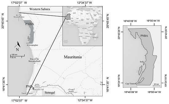
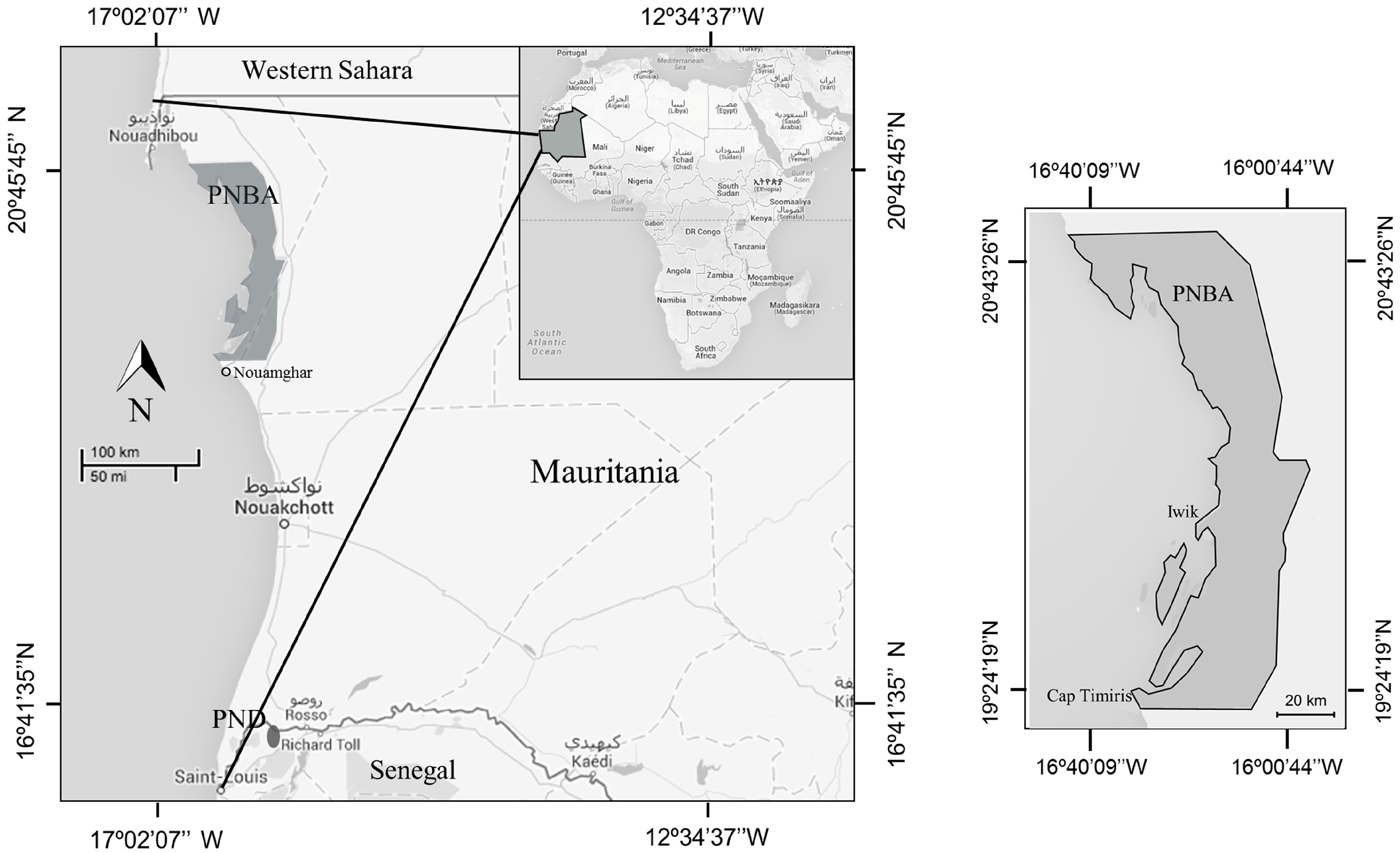
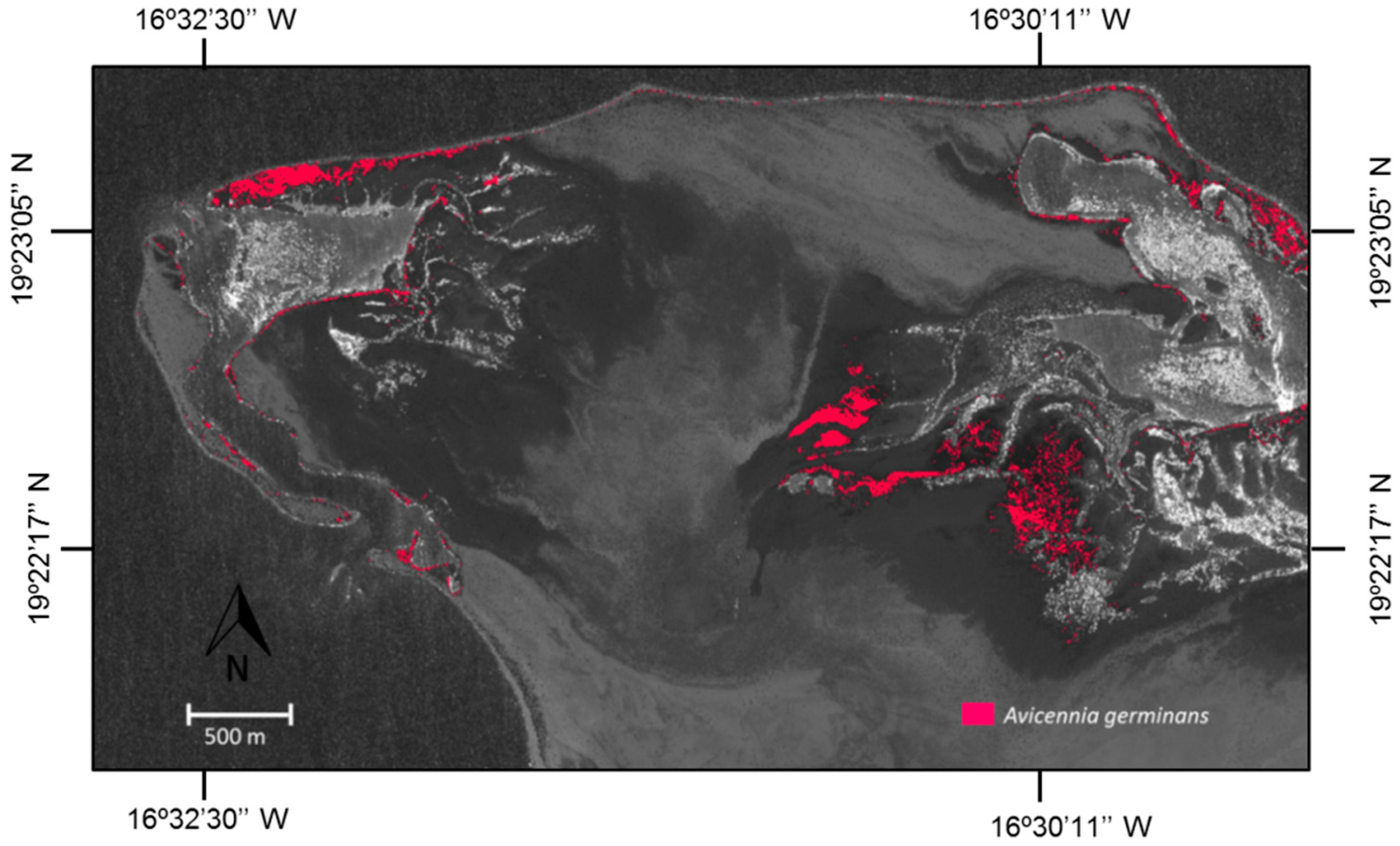
2.1. Study Area

Our case study was done in Cap Timiris, PNBA, Mauritania (Figure 1). Cap Timiris is not the northernmost mangrove assemblage, which is at Iwik, 60 km further North. However, because Cap Timiris has a variety of physiognomical mangrove types, it was chosen for this research. PNBA has been a Ramsar Site since 1982 and a World Heritage Site since 1989 [19,20]. The PNBA area has semidiurnal tides that can reach up to 2 m in height [21]. As for much of the PNBA, the tides may cover large areas of the Cap Timiris area, due to its low elevation. This also generates the high value of the region with its coastal wetlands as stopover areas and wintering areas for migratory birds. Around two million migratory birds are found in this area during the northern winter [12,22,23]. The area has an arid climate [12]. There are no rivers that supply fresh water into the park. Precipitation is estimated to be around 24 mm per year on average [24] and falls between June and October [14]. The rate of evaporation is ten times more than the water income from rainfall, causing high salinity in inshore waters and in the intertidal zone [12].
Due to the arid conditions, the mangrove formations at PNBA have a dwarf growth and a poor regeneration rate [8]. These mangroves have a discontinuous distribution with different physiognomies. Adult trees are found with an average height of 1.2 m, as well as dense shrub formations with a height of 1.4 m [8]. Remarkably enough, however, there are a number of large trees, often isolated, which in certain places aligned along the coastline can reach up to 4.8 m. Finally, there are sebkha-like formations with trees of 0.8 m in height [8]. Coastal dynamics may also affect the extent and health of mangrove stands.
Mangroves are found in assemblages with Arthrocnemum macrostachyum (Moric.) Moris, Salicornia senegalensis A. Chev., Suaeda spp., Sesuvium portulacastrum (L.) L., and Zygophyllum gaetulum Emberger & Maire subsp. waterlotii (Maire) Dobignard, Jacquemoud & Jordan [8]. Additionally, seagrass beds surround the mangroves in tidal flats [14].

2.2. VHR Data and Field Data

Two satellite images of the Cap Timiris area were used (see Table 1). The images had a radiometric, a sensor, and a geometric correction. Both images are projected to a plane with the Universal Transverse Mercator (UTM) coordinate system and are not orthorectified [25]. We used Very High Resolution (VHR) imagery because there are no large extensions of mangrove forest, but small patches and individual trees.
Field data are available from a mission in January of 2009 to PNBA (INCL. Cap Timiris) as a follow-up of an earlier mission in 1998. It consists of (i) a description of the landscape and the vegetation characteristics; (ii) printed maps showing the location of mangroves and other types of terrestrial vegetation in the West side of the study area; and (iii) field photographs of the landscapes. This information was used to select the ground truth data used to train and validate the land cover maps. Landmarks such as big trees and shoreline characteristics were selected as points of reference to select the ground truth data. These landmarks were selected based on the expertise from the field-work and how easily they could be recognized in the satellite images. Although the date of the field work does not correspond exactly to the dates of the images acquisition, the landscape of the study site changes slowly, as reported by one of us having visited the area twice (Nico Koedam in 1998 and 2009) and the selected landmarks from the field work maps were recognizable in both satellite images. Also, the seven month gap in between the months of the year in which both images were taken did not affect the selection of ground truth data and mangrove coverage estimations because of the lack of seasonality in the area and the absence of confusing landmarks.
Data fusion based on the Principal Component Analysis (PCA) technique was performed on both images. After this procedure, the image from 2004 had a spatial resolution of 0.6 m and the image from 2011 had a spatial resolution of 0.5 m. Two supervised classification algorithms were used to map mangroves in Cap Timiris: the Maximum Likelihood Algorithm, commonly used to classify mangroves, and the Neural Network Algorithm Multi-Layer Perceptron, a non-parametric method. The neural network algorithm was trained until the training error started to deviate from the test error. These algorithms were implemented using IDRISI version 17.00 (© Clark University).

2.3. Accuracy Assessment Procedure

Taking into account that a key step in the interpretation of land cover maps is accuracy assessment [26] and several recommendations to perform this assessment appropriately have been proposed [26,27,28,29,30,31], we designed a customized accuracy assessment procedure to verify whether it is possible to detect Cap Timiris’ mangroves unambiguously among other types of land cover using automated classification techniques. We focused on two aspects: (i) how to use the ground truth data and (ii) determining the relevant accuracy metrics for this study.

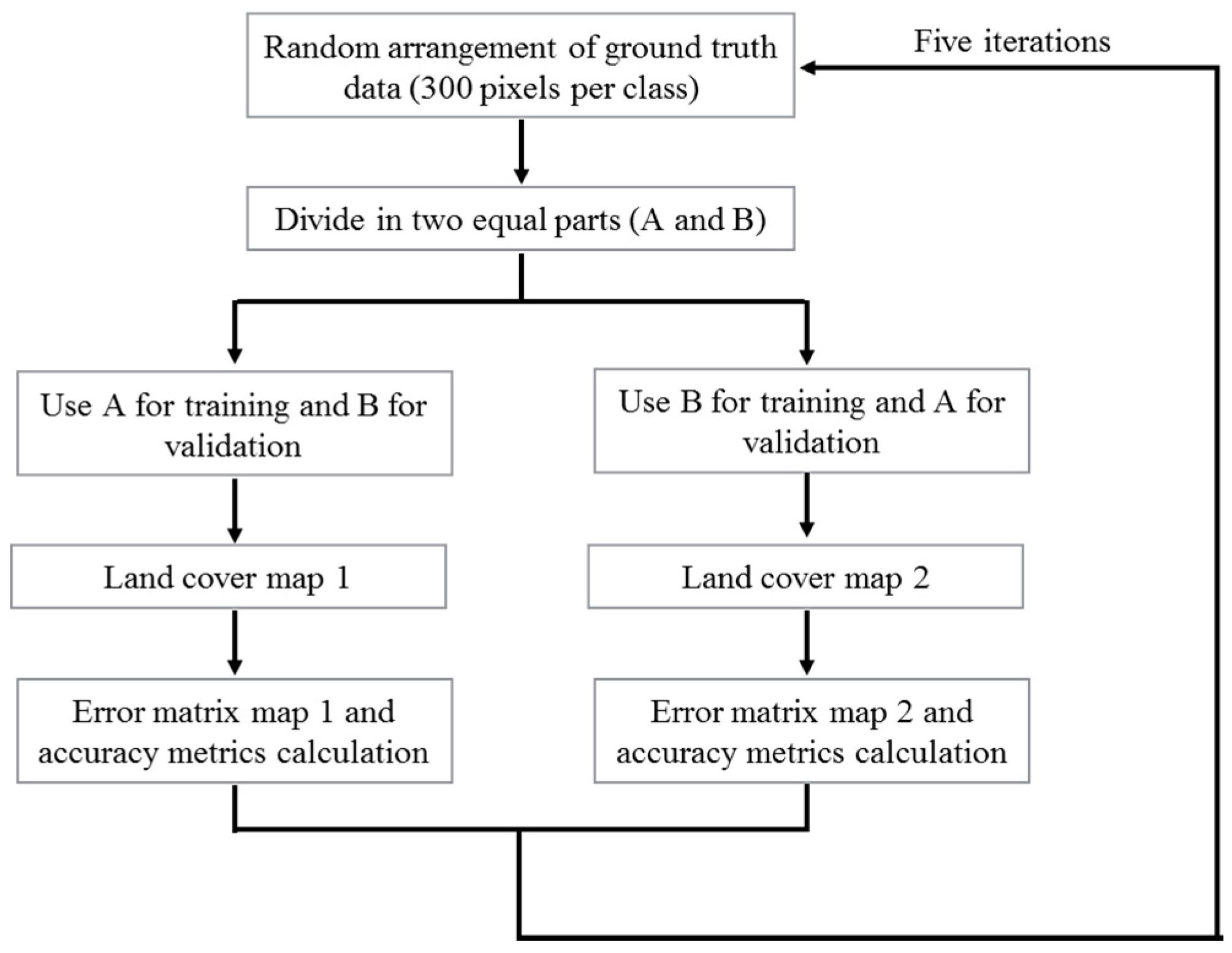
2.3.1. Ground Truth Data

Classifications results can be biased towards the training data [32]. For example, a good accuracy can be obtained if a certain ground truth data set is used, but a different accuracy can be found if another data set is applied in the same satellite image. A way to avoid this bias is by using the cross-validation technique [32]. A cross-validation technique divides a dataset in k subsets of approximately equal size that are mutually exclusive [32]. A classification algorithm is trained using one of the subsets and is validated with the remaining subsets. That step is repeated until all the subsets have been used for training. That procedure is repeated n times using different arrangements of the data [32]. With this method it is possible to observe the effect of the selection of a certain set of training pixels in the classification and accuracy results. Moreover, this technique ensures the same set is never used both for training and validation. The procedure shown in Figure 2 was used to apply the cross-validation technique in this study. The ground truth data is a set of 2100 pixels for each image, where each class is described by 300 pixels. For each iteration in the cross-validation, the ground truth data set is divided randomly in half to create two subsets. One subset will be used for training and the other for validation. Afterwards, the subset used for training in the previous step is used to validate, and the subset used for validation is used for training. This procedure is repeated five times, which means that we performed a twofold cross-validation for five iterations. These iterations produced ten land cover maps and ten error matrices for each classification method (see Figure 2). Even though IDRISI version 17.00 (© Clark University) does not contain a tool to implement this cross-validation technique, we used the Macro-modeler modeling tool to make the five iterations and we used Microsoft Excel to perform the random partition of the ground truth data.
Four important considerations were taken into account for the twofold cross-validation procedure that was repeated five times:
  • We divided the ground truth set in half (twofold) to maximize the number of pixels used for training and validation.
  • We made only five iterations for two reasons: First, there were small differences between each of the ten error matrices among iterations which always reflected the same type of error. Second, the cross-validation was implemented manually using the Macro Modeler of IDRISI, therefore it was a very time consuming task.
  • The training and validation data set for mangroves and other terrestrial vegetation were selected in the West side of the study area because of the availability of field-work information. The bias that can be introduced by this restriction is addressed using the cross-validation technique.
  • Finally, we chose the same amount of pixels per class because the area covered by mangroves in the whole image is about 1%. If we used a stratified random sampling to select the training data, we would have ended up with a very low amount of ground truth data to describe the spectral signature of mangroves as compared to the others types of land cover. The non-mangrove classes were not our main focus of classification and their over-representation might have led to poor classification results for the mangrove category. Olofsson et al. (2013) recommended a procedure to eliminate the bias created by classification errors when calculating the area of a category in a land cover map and report confidence intervals [28]. However, this procedure is only applicable when simple random, systematic or stratified random sampling is used. For this reason, given the characteristics of our area of interest and acknowledging that a bias could have been introduced in the calculation of the area, we used as an alternative the cross-validation technique.

2.3.2. Accuracy Metrics

Each classification algorithm is evaluated with ten error matrices, as a result of the cross-validation procedure. Based on these matrices, we calculated average accuracy and the standard deviation. Moreover, in order to better understand the quality of the classification results, the following metrics were calculated:
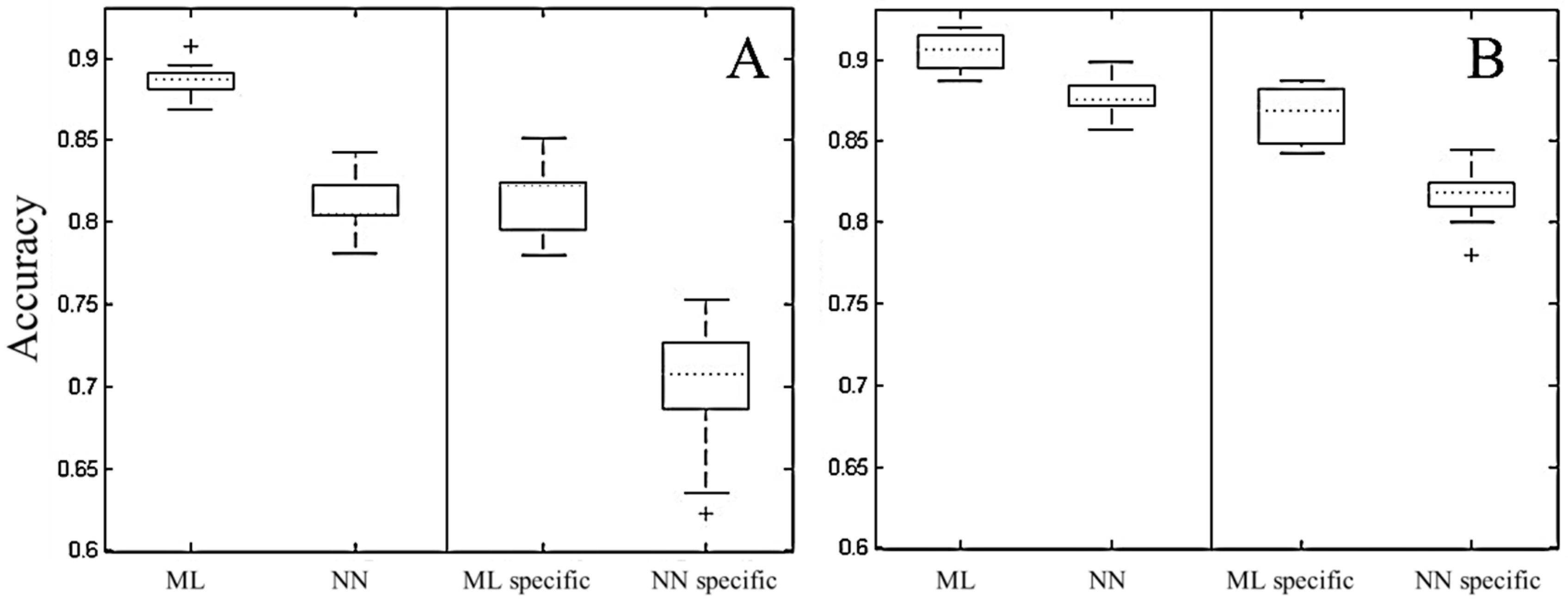
  • A box-plot showing the overall accuracy of the ten error matrices. This accuracy takes into account seven classes of interest (i.e., mangrove, other terrestrial vegetation, sea, shallow water, dry soil, wet soil).
  • A box-plot showing the specific accuracy of the ten error matrices. The specific accuracy only considers three classes of interest: mangrove, other terrestrial vegetation, and other types of land cover. As mentioned before, the area covered by mangroves is very small compared to other types of land cover like soil and shallow water. The specific accuracy is calculated because the overall accuracy can underestimate errors made in the classification of mangroves. Therefore, it is necessary to have a metric that can provide more information about the classification of mangroves and how well the discrimination with other types of vegetation is done. For the classification, seven classes of interest were initially included in order to have more information about the spectral signatures of the different types of land cover.
  • A table showing the commission and omission errors of the ten error matrices.
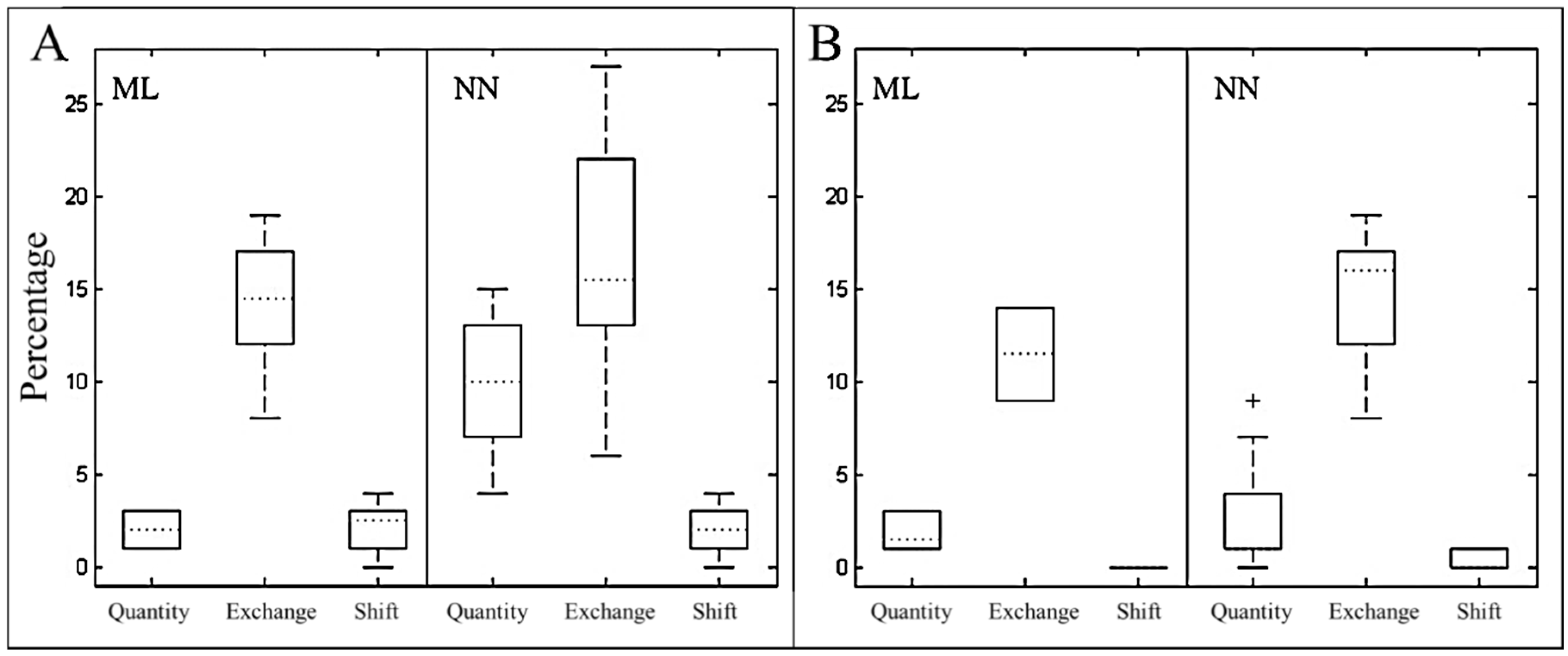
  • A box-plot showing the quantity, exchange, and shift differences of the ten error matrices. These metrics are reported using three classes: mangrove, other terrestrial vegetation, and other types of land cover. Instead of the Kappa Index, Pontius and Millones (2011) and Pontius and Santacruz (2014) propose the use of the quantity, exchange, and shift differences [29,30]. Different authors have suggested that the Kappa Index is not the best option to use as an accuracy assessment metric [27,29]. Quantity refers to the difference, between two land cover maps, in the amount of pixels per category (i.e., class). Exchange refers to the difference in allocation when pixels are interchanged between two categories. Shift refers to other allocation differences that are not included in the exchange difference [29,30]. These metrics are defined based on the error matrix and can be easily calculated with a Microsoft Excel file provided by the authors [30].

3. Results

First, we evaluated whether we could unambiguously detect the mangroves present in Cap Timiris. The highest accuracies were obtained using the Maximum Likelihood Algorithm as compared to the neural network (Figure 3). Furthermore, two additional differences were observed. First, higher accuracies were found in the image from 2011 as compared to the image from 2004. Second, the neural network algorithm had higher variance in the accuracy results compared to the Maximum Likelihood algorithm in the image from 2004.
The omission and commission errors varied between 18% and 38% (Table 2). In the image from 2011 the commission and omission errors were lower in comparison to the image from 2004. Additionally, commission errors were higher than omission errors; in other words, it was more probable to assign a pixel to the mangrove class when it does not truly belong to it.
The main source of error was found in the Exchange Difference (Figure 4). This means, the main error was the interchange of classified pixels between the “mangrove” and the “other terrestrial vegetation” classes. These inaccuracies resulted from the low spectral difference between mangroves and other types of terrestrial vegetation. Moreover, these metrics also showed that higher errors are found in the land cover maps produced with the neural network algorithm as compared to the Maximum Likelihood algorithm.
Moreover, we evaluated the influence of the classification algorithm and the selection of the training pixels in the calculation of the mangrove area (Figure 5). First, there is no agreement between the algorithms in the calculation of the mangrove area for each year. Second, the Maximum Likelihood shows a decrease in area from 2004 to 2011, while the neural network shows an increase. Therefore, the differences in the area calculation between 2004 and 2011 are not a result from actual changes in the mangrove land cover, but a consequence of the selection of the classification algorithm, the training pixels, and misclassification errors.
Based on the previous results, we selected the image from 2011 and the Maximum Likelihood algorithm as the more accurate alternative to map and calculate the mangrove area in Cap Timiris because it has the highest specific accuracy and the lowest commission and omission errors, and quantity, exchange, and shift differences (Figure 6).

4. Discussion

It was possible to map the mangroves of Cap Timiris within other types of land cover using Remote Sensing techniques. However, inaccuracies resulted from the low spectral difference between mangroves and other types of terrestrial vegetation. The highest accuracies were found using the Maximum Likelihood algorithm, which is commonly used for mangrove classification [33,34,35,36,37].
There was a performance difference between the two algorithms used in this study, likely due to the number of parameters that each algorithm had to estimate. Using the same input data set, the Maximum Likelihood algorithm required the estimation of fewer parameters when compared to the neural network algorithm. The Maximum Likelihood had to estimate the mean reflectance and the covariance matrix for each category taking into account four bands. The neural network had to estimate the weights to connect the input, hidden, and output layers. Although the neural network algorithm is more flexible in terms of the statistical distribution of the input data as compared to the Maximum Likelihood algorithm, a limited training data set can affect the accuracy of a neural network classification [38]. In this case study, in particular for mangroves and other types of terrestrial vegetation, the limited amount of input data had an influence in the performance of the algorithms. We also confirm that the Maximum Likelihood algorithm produces higher accuracies, when classifying different mangrove species, compared to the neural network algorithm (cf. [39]).
Furthermore, there were differences between the specific and overall accuracies. The specific accuracy was always lower than the overall one. It was usually observed that the five classes that did not describe terrestrial vegetation (e.g., seawater, dry soil) had higher accuracies than the “mangrove” and “other terrestrial vegetation” classes. These five higher accuracies influenced the overall accuracy hindering the effect of the “mangrove” and “other terrestrial vegetation” inaccuracies. Therefore, the specific accuracy better captured how good an algorithm was (i) to differentiate vegetation from non-vegetation land covers and (ii) to discriminate mangroves from other types of terrestrial vegetation.
The differences in the accuracies calculated for each image could be associated with tidal changes. Even though both images were captured close to the neap tide, a visual inspection of the images shows higher levels of water in 2011 as compared to 2004. Therefore, some areas were wetter or even underwater in 2011, which may also differentiate within the mangrove category (some mangrove areas being flooded at neap tide while others were not). Accordingly, the discrimination of different land covers is easier for the algorithms due to changes in the reflectance patterns. Saito et al. (2003) mapped a mangrove forest in an arid environment and found that changes in tides and water level have more effects on remotely sensed data than rain in this type of environments [36]. Moreover, reflectance patterns of open Avicennia mangrove trees can differ based on the moisture and organic content of the soil in arid environments [40].
The cross-validation technique produced a robust accuracy analysis. It was useful to address the bias introduced by the training data, in particular, by the fact that only ground truth data from the West side was used for the “mangrove” and “other terrestrial vegetation” classes. Therefore, the variation found in the classification algorithms accuracy is optimistic and we could expect even higher variations. To our knowledge, there are no studies that report the use of this technique to evaluate the accuracy for mangrove land cover maps. Yet, the cross-validation technique and another similar one, called bootstrapping, have already been proposed for other applications in Remote Sensing. Brovelli et al. (2008) proposed the cross-validation technique to perform the validation of high resolution satellite images’ orientation accuracy when there are a reduced number of ground truth data points [41]. Franco-Lopez et al. (2001) used cross-validation and bootstrapping techniques to perform the accuracy assessment of the k-nearest neighbors algorithm to calculate cover type, basal area, and volume estimation of a forest in Minnesota, United States [42]. Moreover, Benediktsson et al. (2007) used classifiers that are based on resampling techniques, such as bootstrapping, to analyze multisource remotely sensed data, but not to validate the classification results [43].
Additionally, the metrics proposed by Pontius and Millones (2011) and Pontius and Santacruz (2014) helped to identify specific sources of errors. These metrics showed a differentiation between types of classification errors. We could observe with these metrics that the main classification error was the low differentiation between mangroves and other types of terrestrial vegetation. This is an important source of information in order to evaluate the result of the area calculation. These metrics were also used by Whiteside and Bartolo (2015) to assess the accuracy of a land cover map created for the Magela Creek in Australia, which included mangroves [44].
Mangroves in Mauritania are located in the PNBA and in the Parc National du Diawling [7,12]. Previous estimates of the mangrove cover in Mauritania differ among studies (Table 3). The area estimates found in this study are smaller than the reported values for the whole country [7,14,15,16]. This is logical in the sense that Cap Timiris is part of one of the two areas where mangroves are present in Mauritania. Nevertheless, to our knowledge, there are no reports of Mauritania’s mangrove cover per site, and we could not compare our estimates to other studies. The most reliable estimate for the mangrove area obtained in this study was 19.48 ± 5.54 ha, which was based on the best classification result that was calculated with the Maximum Likelihood algorithm for the image of 2011. However, this value overestimates the area because of the exchange difference errors, and the land cover map obtained in 2011 shows mangroves at the central-east side location where mangroves are not found.
Finally, we showed how the area estimation for a type of land cover can be affected by the selection of the classification algorithm and the training pixels (Figure 5). On the one hand, we found that the amount of input data affected the performance of the neural network and a statistical algorithm such as the Maximum Likelihood performed better under this constraint. On the other hand, the cross-validation technique showed the influence of the selection of the training data on the variation in the area calculated for mangroves. Area calculation for a particular type of land cover is one of the typical applications of land cover maps [27,28]. More emphasis is required on the validation procedure in order to provide a baseline to interpret the results of a land cover map and to calculate estimators for the area quantified with these maps [27,28]. This is a key issue for conservation and land cover monitoring [17,18]. We did not perform a change detection analysis in this study because of the results of the accuracy assessment. This assessment showed that the differences in the mangrove area between 2004 and 2011 are the result of the selection of the classification algorithm, the training data, and misclassification errors instead of a change in the mangrove extension.

5. Conclusions

In this study, we assessed the performance of two Remote Sensing automated classification techniques to map the mangrove formations of Cap Timiris, Mauritania. It was possible to map the mangroves of Cap Timiris within other types of land cover using Remote Sensing techniques. A better classification result was obtained using the Maximum Likelihood algorithm compared to the neural network technique. Furthermore, we found that the selection of the classification algorithm and the training data can affect the classification results.
Additionally, the validation procedure applied in this study was rigorous and novel to map mangroves. Maps created with Remote Sensing classification techniques are potentially used to make policy recommendations and management strategies. Therefore, it is necessary to improve the validation procedure applied on these maps in order to provide contextualized results that can be used in an appropriate way. In this study we accomplished that by using (i) the specific accuracy; (ii) the cross-validation technique; and (iii) the quantity, exchange, and shift differences. Furthermore, software available for Remote Sensing could provide easy to use tools to perform the cross-validation technique or similar type of techniques that support the interpretation of classification results.
It was not possible to calculate a robust estimate of the area covered by mangroves in Cap Timiris. There is high variation in the estimations due to the misidentification of mangroves and other types of terrestrial vegetation. However, improvements in classification might be obtained if other types of remotely sensed data (e.g., hyperspectral data) are used to increase the spectral difference between mangroves and other types of vegetation. It must, however, be emphasized that depending on the successional stage of the mangrove formations and the typology applied, inclusion or omission may follow. Indeed, extensive areas of juvenile cohorts may exist, as yet undetectable by remote sensing, while on the other hand shrub-like Avicennia germinans may be distributed amongst equally high halophytic vegetation of, for example, Arthrocnemum macrostachyum. High resolution detection of local vegetation dynamics will still require field monitoring.
Finally, the relevance of Remote Sensing to monitor and provide baseline information about mangroves is not in question. In this study, it was possible to detect the northernmost continuous mangroves patches of West Africa with an accuracy of 87% ± 2% using the Maximum Likelihood algorithm. In spite of the shortcomings found in the classification results, our validation procedure allowed us to report the exact sources of errors of the classification maps and address the bias introduced by the training data. Therefore, useful information can be provided for the management of Mauritania’s mangroves based on the accurate assessment of the classification results. Moreover, this validation procedure is also useful for other areas where latitudinal mangroves are found in similar arid climate conditions (e.g., Egypt, Iran, Peru, Saudi Arabia) [7].

Acknowledgments

The field work in 2009 was financed by the Leopold-III Foundation and the Belgian National Research Foundations (FWO and FNRS). The research was also funded by a Mandat d’Impulsion Scientifique (MIS) from FNRS, and by the Belgian Royal Academy of Overseas Sciences. We are grateful to the staff of the PNBA, Diana Di Nitto, Stefano Cannicci, and Fabrizio Bartolini for facilitating field-work logistics through a joint mission in 2009. This paper is published with the support of the Belgian University Foundation. Publié avec le concours de la Fondation Universitaire de Belgique.

Author Contributions

Farid Dahdouh-Guebas designed the topic and acquired the images; Katrien Quisthoudt and Nico Koedam carried out fieldwork in 2009, and Farid Dahdouh-Guebas and Nico Koedam in 1998; Viviana Otero carried out the Remote Sensing analysis and analyzed fieldwork data; Farid Dahdouh-Guebas , Nico Koedam, and Katrien Quisthoudt supervised the research; Farid Dahdouh-Guebas, Nico Koedam, and Viviana Otero conceived and designed the methods; Viviana Otero wrote the manuscript with major contributions of all co-authors.

Conflicts of Interest

The authors declare no conflict of interest.

Abbreviations

The following abbreviations are used in this manuscript:
MLMaximum Likelihood algorithm
NNNeural Network algorithm
PANPanchromatic band
PCAPrincipal Component Analysis
PNBAParc National du Banc d’Arguin
PNDParc National du Diawling
UTMUniversal Transverse Mercator
VHRVery High Resolution
XSMultispectral band

References

  1. Gaston, K.J. Geographic range limits of species. Proc. R. Soc. 2009, 276, 1391–1393. [Google Scholar] [CrossRef] [PubMed]
  2. Sexton, J.; McIntyre, P.J.; Angert, A.L.; Rice, K.J. Evolution and ecology of species range limits. Annu. Rev. Ecol. Evol. Syst. 2009, 40, 415–436. [Google Scholar] [CrossRef]
  3. Thuiller, W. BIOMOD—Optimizing predictions of species distributions and projecting potential future shifts under global change. Glob. Chang. Biol. 2003, 9, 1353–1362. [Google Scholar] [CrossRef]
  4. Mukherjee, N.; Sutherland, W.J.; Khan, M.N.I.; Berger, U.; Schmitz, N.; Dahdhouh-Guebas, F.; Koedam, N. Using expert knowledge and modeling to define mangrove composition, functioning, and threats and estimate time frame of recovery. Ecol. Evol. 2014, 4, 2247–2262. [Google Scholar] [CrossRef] [PubMed]
  5. Duke, N.C.; Ball, M.C.; Ellison, J.C. Factors influencing biodiversity and distributional gradients in mangroves. Glob. Ecol. Biogeogr. Lett. 1998, 7, 27–47. [Google Scholar] [CrossRef]
  6. Ellison, A. Macroecology of mangroves: Large-scale patterns and processes in tropical coastal forests. Trees 2002, 16, 181–194. [Google Scholar] [CrossRef]
  7. Spalding, M.; Kainuma, M.; Collins, L. World Atlas of Mangroves; Earthscan: London, UK, 2010. [Google Scholar]
  8. Dahdouh-Guebas, F.; Koedam, N. Are the northernmost mangroves of West-Africa viable?—A case study in Banc d’Arguin National Park, Mauritania. Hydrobiologia 2001, 458, 241–253. [Google Scholar] [CrossRef]
  9. Saintlan, N.; Rogers, K.; McKee, K. Salt marsh-mangrove interactions in Australasia and the Americas. In Coastal Wetlands: An Integrated Ecosystem Approach; Elsevier: Amsterdam, The Netherlands, 2009. [Google Scholar]
  10. Duke, N.C. Australia’s Mangroves. In The Authoritative Guide to Australia’s Mangrove Plants; University of Queensland: Brisbane, Australia, 2006. [Google Scholar]
  11. Quisthoudt, K.; Schmitz, N.; Randin, C.F.; Dahdouh-Guebas, F.; Robert, E.M.R.; Koedam, N. Temperature variation among mangrove latitudinal range limits worldwide. Trees 2012, 26, 1919–1931. [Google Scholar] [CrossRef]
  12. Blasco, F. About the mangroves of Banc d’Arguin, Mauritania. ISME/GLOMIS Electron. J. 2010, 8, 13–15. [Google Scholar]
  13. Giri, C.; Ochieng, E.; Tieszen, L.L.; Zhu, Z.; Singh, A.; Loveland, T.; Masek, J.; Duke, N. Status and distribution of mangrove forest of the world using earth observation satellite data. Glob. Ecol. Biogeogr. 2011, 20, 154–159. [Google Scholar] [CrossRef]
  14. Lamarche, S. Cartographie et Répartition de la Végétation du Cap Timiris; Observatoire du Parc National du Banc d’Arguin: Nouadhibou, Mauritania, 2008. [Google Scholar]
  15. United Nations Environment Programme (UNEP). Mangroves of Western and Central Africa; UNEP Regional Seas Programme/UNEP—World Conservation Monitoring Centre (WCMC): Cambridge, UK, 2007. [Google Scholar]
  16. Fatoyinbo, T.E.; Simard, M. Height and biomass of mangroves in Africa from ICESat/GLAS and SRTM. Int. J. Remote Sens. 2013, 34, 668–681. [Google Scholar] [CrossRef]
  17. Turner, W.; Spector, S.; Gardiner, N.; Fladeland, M.; Sterling, E.; Steininger, M. Remote sensing for biodiversity science and conservation. Trends Ecol. Conserv. 2003, 18, 306–314. [Google Scholar] [CrossRef]
  18. Kerr, J.T.; Ostrovsky, M. From space to species: Ecological applications for remote sensing. Trends Ecol. Conserv. 2003, 18, 299–305. [Google Scholar] [CrossRef]
  19. United Nations Educational, Scientific and Cultural Organization (UNESCO), World Heritage Convention. State of Conservation: Banc d’Arguin National Park 2013. Available online: http://whc.unesco.org/en/soc/1924 (accessed on 5 March 2016).
  20. Ramsar Convention on Wetlands. Ramsar Sites Information Service. Available online: https://rsis.ramsar.org/ris/250 (accessed on 5 March 2016).
  21. Van der Laan, B.P.A.; Wolff, W.J. Circular pools in the seagrass beds of the Banc d’Arguin, Mauritania, and their possible origin. Aquat. Bot. 2006, 84, 93–100. [Google Scholar] [CrossRef]
  22. Hagemeijer, W.; Smit, C.; de Boer, P.; Van Dijk, A.; Ravenscroft, N.; Van Roomen, M.; Wright, M. Wader and Waterbird Census at the Banc d’Arguin, Mauritania, January 2000; IWO Report 81; Foundation Working Group International Waterbird and Wetland Research (WIWO): Nijmegen, The Netherlands, 2004; pp. 3–141. [Google Scholar]
  23. Leyrer, J.; Spaans, B.; Camara, M.; Piersma, T. Small home ranges and high site fidelity in red knots (Calidris c. canutus) wintering on the Banc d’Arguin, Mauritania. J. Ornithol. 2006, 147, 376–384. [Google Scholar] [CrossRef]
  24. Dia, A.T.; Colas, F.; De Wispelaere, G. Contribution à L’étude des Milieux Naturels du Littoral Mauritanien. In Proceedings of the Environnement at Littoral Mauritanien: Actes du Colloque, Nouakchott, Mauritanie, Montpellier, France, 12–13 June 1995.
  25. DigitalGlobe. Standard Imagery Datasheet. Available online: http://global.digitalglobe.com/sites/default/files/StandardImagery-DS-STAND_1-22-14_0.pdf (accessed on 3 March 2016).
  26. Foody, G.M. Status of land cover classification accuracy assessment. Remote Sens. Environ. 2002, 80, 185–201. [Google Scholar] [CrossRef]
  27. Olofsson, P.; Foody, G.M.; Herold, M.; Stehman, S.V.; Woodcock, C.E.; Wulder, M.A. Good practices for estimating area and assessing accuracy of land change. Remote Sens. Environ. 2014, 148, 42–57. [Google Scholar] [CrossRef]
  28. Olofsson, P.; Foody, G.M.; Stehman, S.; Woodcock, C.E. Making better use of accuracy data in land change studies: Estimating accuracy and area and quantifying uncertainty using stratified estimation. Remote Sens. Environ. 2013, 129, 122–131. [Google Scholar] [CrossRef]
  29. Pontius, R.G.; Millones, M. Death to Kappa: Birth of quantity disagreement and allocation disagreement for accuracy assessment. Int. J. Remote Sens. 2011, 32, 4407–4429. [Google Scholar] [CrossRef]
  30. Pontius, R.G.; Santacruz, A. Quantity, exchange, and shift components of difference in a square contingency table. Int. J. Remote Sens. 2014, 35, 7543–7554. [Google Scholar] [CrossRef]
  31. Stehman, S.V. Sampling designs for accuracy assessment of land cover. Int. J. Remote Sens. 2009, 30, 5243–5272. [Google Scholar] [CrossRef]
  32. Kohavi, R. A study of cross-validation and bootstrap for accuracy estimation and model selection. In Proceedings of the International Joint Conference on Artificial Intelligence (IJCAI), Montreal, QC, Canada, 20–25 August 1995.
  33. Gao, Y. A comparative study on spatial and spectral resolution of satellite data in mapping mangrove forests. Int. J. Remote Sens. 1999, 20, 2823–2833. [Google Scholar] [CrossRef]
  34. Kuenzer, C.; Bluemel, A.; Gebhardt, S.; Quoc, T.V.; Dech, S. Remote sensing of mangrove ecosystems: A review. Remote Sens. 2011, 3, 878–928. [Google Scholar] [CrossRef]
  35. Satyanarayana, B.; Mohamad, K.A.; Idris, I.F.; Husain, M.; Dahdouh-Guebas, F. Assessment of mangrove vegetation based on remote sensing and ground-truth measurements at Tumpat, Kelantan Delta, East Coast of Peninsular Malaysia. Int. J. Remote Sens. 2011, 32, 1635–1650. [Google Scholar] [CrossRef]
  36. Saito, H.; Bellan, M.F.; Al-Habshi, A.; Aizpuru, M.; Blasco, F. Mangrove research and coastal ecosystem studies with SPOT-4 HR VIR and TERRA ASTER in Arabian Gulf. Int. J. Remote Sens. 2003, 24, 4073–4092. [Google Scholar] [CrossRef]
  37. Wang, L.; Sousa, W.P.; Gong, P. Integration of object-based and pixel-based classification for mapping mangroves with IKONOS imagery. Int. J. Remote Sens. 2004, 25, 5655–5668. [Google Scholar] [CrossRef]
  38. Foody, G.M.; Arora, M.K. An evaluation of some factors affecting the accuracy of classification by an artificial neural network. Int. J. Remote Sens. 1997, 18, 799–810. [Google Scholar] [CrossRef]
  39. Wang, L.; Silván-Cárdenas, J.L.; Sousa, W.P. Neural Network Classification of Mangrove Species from Multi-Seasonal Ikonos Imagery. Photogramm. Eng. Remote Sens. 2008, 74, 921–927. [Google Scholar] [CrossRef]
  40. Al Habshi, A.; Youssef, T.; Aizpuru, M.; Blasco, F. New mangrove ecosystem data along the UAE coast using remote sensing. Aquat. Ecosyst. Health Manag. 2007, 10, 309–319. [Google Scholar] [CrossRef]
  41. Brovelli, M.A.; Crespi, M.; Fratarcangeli, F.; Giannone, F.; Realini, E. Accuracy assessment of high resolution satellite imagery orientation by leave-one-out method. ISPRS J. Photogramm. Remote Sens. 2008, 63, 427–440. [Google Scholar] [CrossRef]
  42. Franco-Lopez, H.; Ek, A.R.; Bauer, M.E. Estimation and mapping of forest stand density, volume and cover type using the k-nearest neighbors method. Remote Sens. Environ. 2001, 77, 251–274. [Google Scholar] [CrossRef]
  43. Benediktsson, J.A.; Chanussot, J.; Fauvel, M. Multiple Classifier Systems in Remote Sensing: From Basics to Recent Developments. In Proceedings of the Multiple Classifier Systems, 7th International Workshop, MCS 2007, Prague, Czech Republic, 23–25 May 2007.
  44. Whiteside, T.G.; Bartolo, R.E. Mapping aquatic vegetation in a tropical wetland using high spatial resolution multispectral satellite imagery. Remote Sens. 2015, 7, 11664–11694. [Google Scholar] [CrossRef]
Figure 1. The study site Cap Timiris at Parc National du Banc d’Arguin (PNBA), Mauritania. The Iwik area and the Parc National du Diawling (PND) are also indicated (see text). Adapted from Google Maps (2016).
Remotesensing 08 00512 g001
Figure 2. Procedure used to select the pixels for training and validation in the supervised classification based on the cross-validation technique.
Remotesensing 08 00512 g002
Figure 3. Box-plot of the accuracies for the Maximum Likelihood (ML) and neural network (NN) algorithms implemented for the image from 2004 (A) and 2011 (B). The overall accuracies are named “ML” and “NN”. The specific accuracies are named “ML specific” and “NN specific”. These results were obtained with the five iterations of the cross-validation technique.
Remotesensing 08 00512 g003
Figure 4. Box-plot showing the quantity, exchange, and shift differences of the image from 2004 (A) and 2011 (B). ML refers to the Maximum Likelihood and NN to the neural network algorithm. These metrics were calculated taking into account the specific accuracy.
Remotesensing 08 00512 g004
Figure 5. Area (Ha) calculated with Maximum Likelihood Algorithm (ML) and the neural network (NN) for the image from 2004 (A) and in 2011 (B).
Remotesensing 08 00512 g005
Figure 6. Mangroves at Cap Timiris, since mangroves in PNBA only comprise the mangrove species Avicennia germinans. There is an overestimation of mangroves in the central-east part of the area, mangroves are not found in that location.
Remotesensing 08 00512 g006
Table 1. Resolution specifications of the satellite images. PAN refers to the panchromatic band and XS to the multispectral bands. B refers to blue, G to green, R to red, and NIR to near-infrared.
CharacteristicQuickBird Sensor (2004)GeoEye Sensor (2011)
Date and time of acquisition23 December 2004 at 11:46 GMT21 July 2011 at 11:51 GMT
Spatial resolutionPAN: 0.6 mPAN: 0.5 m
XS: 2.4 mXS: 2 m
Spectral resolutionB: 430–545 nmB: 450–510 nm
G: 466–620 nmG: 510–580 nm
R: 590–710 nmR: 655–690 nm
NIR: 715–918 nmNIR: 780–920 nm
Radiometric resolution11 bits per pixel11 bits per pixel
Temporal resolutionLess than 3 daysLess than 3 days
Table 2. Omission and commission errors for the “mangrove” class for the images from 2004 and 2011. The results for the Maximum Likelihood and the neural network algorithms are shown individually. The results were obtained with the five iterations of the cross-validation technique.
AlgorithmType of Error20042011
Maximum LikelihoodOmission error22% ± 5%18% ± 6%
Commission error28% ± 3%20% ± 1%
Neural NetworkOmission error20% ± 8%25% ± 9%
Commission error38% ± 3%26% ± 4%
Table 3. Available mangrove area estimations in Mauritania.
StudyMangrove Area
UNEP (2007) [15]100 ha in 2000 and 209 ha in 2006 (total area in Mauritania)
Lamarche (2008) [14]400 ha at Cap Timiris and Tidra Island in 2007
Spalding et al. (2010) [7]139 ha (total area in Mauritania)
Fatoyinbo and Simard (2013) [16]40 ha between 1999 and 2000 (total area in Mauritania)
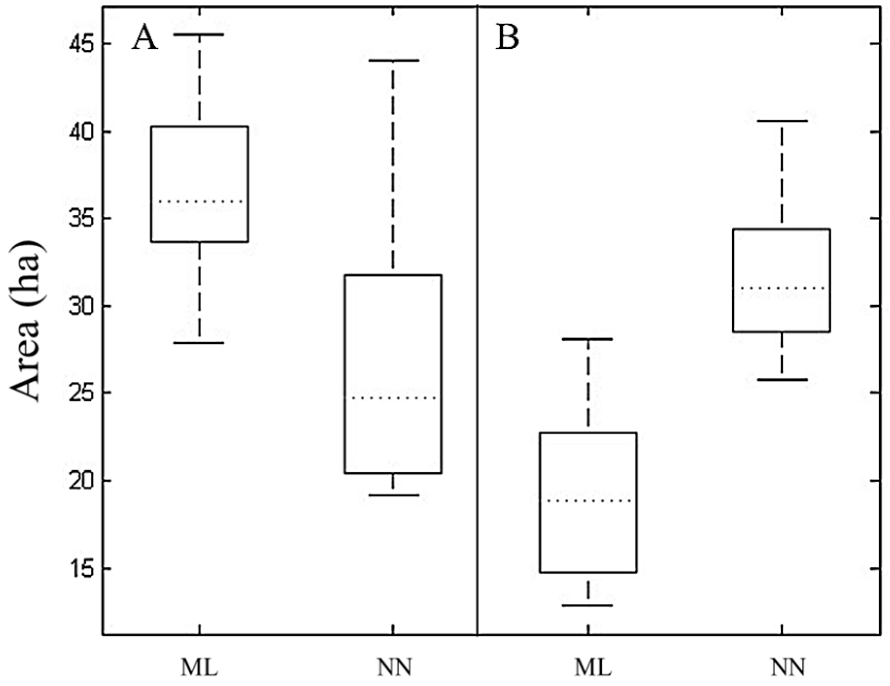
This study19.48 ± 5.54 ha in Cap Timiris in 2011

