Article

Submerged Kelp Detection with Hyperspectral Data

1
Department of Geography, Kiel University, Ludewig-Meyn-Str. 14, Kiel 24118, Germany
2
Alfred-Wegener-Institute, Helmholtz Centre for Polar and Marine Research, Am Handelshafen 12, Bremerhaven 27570, Germany
*
Author to whom correspondence should be addressed.
Remote Sens. 2016, 8(6), 487; https://doi.org/10.3390/rs8060487
Submission received: 31 March 2016 / Revised: 30 May 2016 / Accepted: 2 June 2016 / Published: 8 June 2016
(This article belongs to the Special Issue Remote Sensing in Coastal Environments)

Abstract

:
Submerged marine forests of macroalgae known as kelp are one of the key structures for coastal ecosystems worldwide. These communities are responding to climate driven habitat changes and are therefore appropriate indicators of ecosystem status and health. Hyperspectral remote sensing provides a tool for a spatial kelp habitat mapping. The difficulty in optical kelp mapping is the retrieval of a significant kelp signal through the water column. Detecting submerged kelp habitats is challenging, in particular in turbid coastal waters. We developed a fully automated simple feature detection processor to detect the presence of kelp in submerged habitats. We compared the performance of this new approach to a common maximum likelihood classification using hyperspectral AisaEAGLE data from the subtidal zones of Helgoland, Germany. The classification results of 13 flight stripes were validated with transect diving mappings. The feature detection showed a higher accuracy till a depth of 6 m (overall accuracy = 80.18%) than the accuracy of a maximum likelihood classification (overall accuracy = 57.66%). The feature detection processor turned out as a time-effective approach to assess and monitor submerged kelp at the limit of water visibility depth.

Graphical Abstract

1. Introduction

Kelp ecosystems dominate approximately 25% of the world’s rocky shores [1]. Kelps belong to the brown algae of the order Laminariales and form submerged forests of macroalgae. They are one of the key structures in worldwide coastal ecosystems and of great importance for ecosystem functions, aquaculture and food industries [2,3]. Kelp is relevant in determining patterns of abundance and food supply for fish and invertebrates [4]. Its occurrence is strongly related to the resources required by different life history stages of fish populations, providing foraging habitat and spatial refuge from predators [5]. Kelp also has a growing economic value and is harvested for human food consumption as well as being used in the alginate, mannitol and iodine industry [6,7]. The high biological productivity, fast growth and high polysaccharide content make macroalgae and, therefore, also kelp forests attractive for biofuel production [8]. Thus, these harvested patterns and human uses can affect coastal ecosystems and economies.
Kelp is a sessile life form and constitutes persistent mats or three-dimensional forests in the coastal eutrophic subtidal zones. The forests flourish from the low tide level up to a depth of 20–30 m, depending on the turbidity of coastal zones [9]. The species vary considerably in form and size. In the N-Atlantic kelp species often grow to about 2–3 m in length [10] and forests have to be tolerant to the physical conditions of their environment, i.e., diurnal or seasonal variations in temperature, salinity, water movement, nutrient and carbon delivery, light availability and levels of UV radiation [11]. Kelps are rather stenothermal and adapted to a narrow range of environmental conditions [12]. Thus, changes in the occurrence of kelp indicate changing environmental and habitat conditions caused e.g., by increasing water temperatures or sea level rise [13].
Kelp ecosystems are responding to climate driven habitat changes all over the world (e.g., Japan: [14], Tasmania: [15], Norway: [16,17], Spain: [18]). In many temperate regions, kelp forests are retreating due to ocean warming and human pressure [19,20]. Several modelling studies forecast a poleward shift of benthic marine species [21,22,23]. Recent field evidence also suggests that Arctic kelp ecosystems are currently undergoing change. At one site in Spitsbergen the depth distribution of kelps was found to be becoming shallower and biomass has increased considerably [16]. Possible driving forces are strongly connected to climate change, e.g., the change of the underwater irradiance climate, a lack of ice-scouring in winter, the elongation of the open-water period and increased sedimentation [16]. These climate driven changes and the concomitant threats to the marine flora and fauna are considered by the European Marine Strategy Framework Directive. Programs of measures for the protection and management of the marine environment should be implemented considering scientific and technological developments [24].
Rocky shore communities are highly suitable for long-term ecological studies and appropriate indicators of ecosystem health [25]. Most studies, however, have been conducted in intertidal habitats that are easily accessible but strongly influenced by tides and waves [26]. Few studies monitor subtidal habitats with canopy-forming macroalgae such as kelp, mainly because they are difficult to sample [27]. Remote sensing methods gather areal information about these habitats with less cost intensive field data sampling. In recent years, techniques have been developed for benthic mapping in clear waters [28,29,30,31,32]. Some studies also achieved promising results for mapping marine bottom types in turbid waters, e.g., [33,34]. A poor penetration of light into the water column however was the major limitation factor.
The difficulty in analysing submerged plants is that their spectral reflectance is usually very low because water strongly absorbs electromagnetic radiation in the optical spectral region [35,36]. Experimental studies have shown that the contribution of submerged aquatic vegetation (SAV) to the measured remote sensing signal decreases with increasing depth of the water column over the vegetation, resulting in a diminished spectral signal of the target species [37], whereas absolute reflectances of emergent macroalgae, like kelp and other brown algae, significantly increase with desiccation [38]. Further variability is introduced by changing water levels during tides and due to currents resulting in a mixing of plant and water signal [39]. Optically active water components, such as suspended solids or chlorophyll, may share spectral features with SAV [40]. The spectral signature of aquatic vegetation therefore shows overlapping signatures from water resulting in a wide range of reflectance values impeding classification [41].
Satellite-borne systems are particularly suitable for long-term monitoring due to their high temporal resolution. Several studies use multispectral satellite systems to achieve information about SAV (e.g., [42,43,44]), but remote sensing of benthic ecosystems can only make use of spectral bands in the wavelengths at approximately 400–740 nm which penetrate into the water [45]. The narrow bandwidths of forthcoming hyperspectral missions like EnMAP [46] or PRISMA [47] provide a better spectral resolution in the visible wavelength range. This enables the detection of local features for kelp and macroalgae detection in general [48]. Unfortunately, these systems are still unavailable and suitable approaches currently can only be developed using airborne hyperspectral systems. The airborne systems have already been shown to be suitable for mapping seagrass species, cover and biomass in clear shallow waters [49] and to differentiate between macroalgae and floating seagrass mats [50]. The development of new methods should therefore ensure transferability to satellite-borne systems.
In the present study, we developed a fully automated simple processor to detect the presence of kelp from airborne hyperspectral AisaEAGLE data. The algorithm is designed to work without the need of field data or intense training. The approach consists of three steps: (1) an anomaly filter to remove effects on the water surface; (2) a derivative-based algorithm for kelp-feature extraction and (3) an identification of kelp dominated pixels using specific spectral features of kelps. The aim of this algorithm is to reduce the depth limitations imposed by reflectance-based classification methods. Therefore, we compare the results with a common maximum likelihood classification without anomaly filtering.

2. Materials and Methods
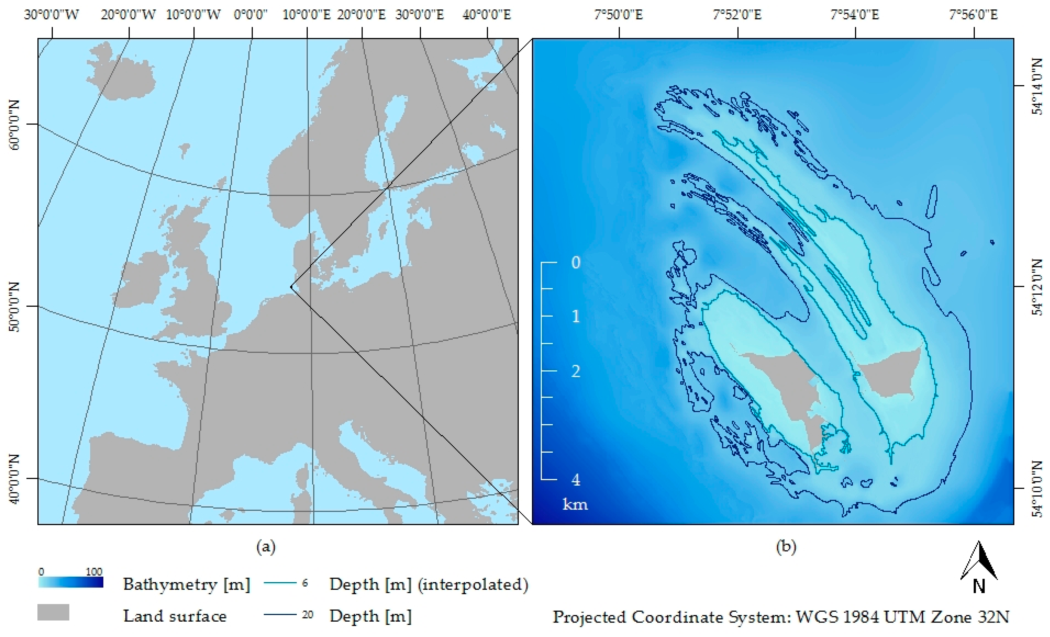
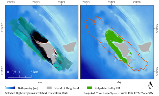
2.1. Study Site

The archipelago of Helgoland (54°11′N, 7°53′E) is located 50 km off the German coastline in the central German Bight (North Sea) (Figure 1a). It is the only terrestrial site in this region with an offshore character [51]. Helgoland is divided into two small islands: the main rocky red sandstone island Helgoland with an areal coverage of 1.1 km2 and the smaller sandy dune island with 0.6 km2. The subtidal zone around the two islands is the only hard-bottom locality in the south-eastern part of the North Sea [52]. The region is characterized by an offshore climate with perennial rainfall (average annual precipitation = 752 mm) and low annual air temperature fluctuations (daily mean = 9.8 °C) [53]. According to Franke et al., (2004) observed changes in the composition of subtidal macroalgae communities may indicate a climate shift from North Sea climate towards more oceanic conditions (higher mean winter water temperature, higher and more constant salinities) [54].
The study site is the subtidal of the archipelago demarcated by the 20-metre isobaths derived from a bathymetric map from the Federal Maritime and Hydrographic Agency of Germany (Figure 1). This map is the basis to estimate the depth of the detected kelp patches in this study. The map has five depth classes between 0 and 20 m: >0 m; 0–2 m; 2–5 m; 5–10 m and 10–20 m. We also interpolated these classes to achieve a second infinitely variable depth map (Figure 1b). The bottom substrates along Helgoland’s shore are red sandstone, chalk and flint stone. The rocky seafloor forms an eroded terrace north and west of the main island. Significant beach nourishments in the early twentieth century moulded the natural rock base south and east of the main island. Nevertheless, the characteristic morphology of the rocky substratum still offers numerous small habitats as an ideal environment for highly diverse macroalgae communities [55]. Extensive kelp forests of the brown algae species Laminaria digitata, Laminaria hyperborea, Saccharina latissima and Desmarestia aculeata dominate the subtidal zone. They are accompanied by an understorey of red algae, e.g., Delesseria sanguinea, Plocamium cartilagineum or Polysiphonia sp. The solid substrates in the subtidal are nearly always covered by algae [56]. Brown algae of the species Fucus serratus form dense canopies on the intertidal sandstone ridges, but their occurrence ends at the infralittoral zone [57]. The high turbidity of the waters around Helgoland limits the lower growth limit of Laminariales at about 8–10 m, whereas red-algae still occur in depths up to 20 m [9,56].

2.2. Field Survey

Mapping via diving transects is a well-established method to investigate subtidal zones [56,58]. For this study, we used georeferenced transect diving mappings conducted during two intensive field campaigns in summer 2010 and 2011 (Figure 2) which serve as reference for our remote sensing study. As the subtidal kelp forest is mostly built up by the perennial kelp Laminaria hyperborea [56,58], there is considerable stability over time in the presence of the forest [56,59]. Thus, the diving information of both years was used here as validation reference for the remote sensing study.
Data were collected at regular intervals along a horizontal line at the sea floor and species presence/absence and abundances were recorded. The divers recorded the algal cover approximately every six meters. The distance was measured with the help of a 2 m stick. The precision of this underwater distance measurement is not comparable with land measurements and is influenced by drift and water movement. Therefore, the distance of the recorded points generally varied between 5 m and 10 m but was sometimes even bigger explaining the partially observable gaps in the diving ground truth information (Figure 2). Geo-referencing was achieved in the following way: the divers carried a buoy with an attached Magellan GPS 320 receiver to achieve point location information for their measurements. At regular distances, the line holding the buoy was pulled straight above the head of the diver and later the subtidal position was correlated via the synced time stamps of the GPS and the diving computer. Figure 2 illustrates the spatial distribution of transects in the study area.
Measurements were conducted every six metres (mapping radius three metres) and included:
  • Cover estimation of the four dominant brown macroalgae (Laminaria digitata, Laminaria hyperborea, Saccharina latissima, Desmarestia aculeata).
  • Presence/absence of brown algae Water depth measurement using a digital depth gauge (Seemann Sub; precision: 40 cm) and transferred to sea chart level zero [56].
A detailed description of the diving data acquisition is published by Pehlke and Bartsch (2008) [56]. Altogether, the divers mapped 21 transects during the two campaigns. The mapped data were transferred into a Geographical Information System (GIS). The depth measures were converted to sea chart level zero with help of the tide gauge level data Helgoland [60]. Coinciding with the mappings we documented the status of the main kelp habitats with photographs.
The diving mappings only capture the subtidal areas of the study area. We used intertidal field mappings in addition to the diving data for the validation of the remote sensing classifications results in shallow waters [41,61]. The intertidal areas are mainly dominated by brown algae from the order Fucales. These mappings in combination with digital orthophotos enable an evaluation of whether the classification methods successfully separate kelp habitats from Fucales habitats in the shallow waters of the study area.

2.3. Hyperspectral Data

The remote sensing data of the study site was acquired using a hyperspectral AisaEAGLE system. The progressive scan CCD detector system consists of a high efficiency transmissive imaging spectrograph, a diffuse down welling irradiance collector (FODIS), an Oxford RT3100 global positioning system (GPS), inertial measurement unit (IMU) (position accuracy ≥ 1.8 m) and a computer for data storage and system control [62,63]. The radiometric resolution of the spectrograph is 12 bit for up to 488 spectral bands within a spectral range of 400–900 nm and with a spectral sampling rate of 3.3 nm. To gain a better signal to noise ratio the sensor was set to a spectral binning of four resulting in 120 spectral bands with a sampling rate of 4.6 nm. Furthermore, a spatial binning of two produced 512 pixels across track. Altogether, thirteen flight stripes were recorded on 9 May 2008 (Figure A1) with a motor glider Condor Stemme S10 owned by Orbital High-technology Bremen (OHB System AG). Data acquisition took place between 10:00 and 11:45 h UTC at low tide under sunny and calm conditions at an altitude of 693 m (2300 ft) above sea level and a velocity of 31 m/s (112 km/h) (Table 1). The resulting pixel spacing is 0.92 m along track and 0.68 m across track.
The AISA data were radiometrically pre-processed and calibrated using the software CaliGeoPro [62]. Geometric correction was conducted using the GPS/IMU data acquired during the flight and boresight calibration measurements. The pixels were afterwards resampled to 1 × 1 m pixel spacing using the nearest neighbour approach. The radiometric pre-processing included a dark current correction and a sensor calibration using data provided by SPECIM. At-Sensor reflectances were obtained using the FODIS measurements. The next step of data processing was an atmospheric correction to surface reflectance using ATCOR-4 [64]. Tec5 HandySpec [65] (spectral range 350–950 nm, spectral sampling interval 3 nm) field spectrometer data collected during the AISA data acquisition were used to validate the AISA reflectance values. We further masked land and emergent surfaces using a reflectance threshold at 957 nm and further flagged pixels with a reflectance higher than 3% and 10%, respectively. The WAF algorithm is written with the programming language IDL for the software EnMAP-Box [66].

2.4. Kelp Detection

We developed and applied a fully automatic processor to detect the presence or absence of kelp in remote sensing images of subtidal rocky coastal shores. The program is divided into two steps: at first a Water Anomaly Filter (WAF) is applied to prepare the data for the kelp analysis and, secondly, a spectral kelp feature detection was used to separate kelp pixels from non-kelp pixels.

2.4.1. Water Anomaly Filter—WAF

WAF is a spatial function to remove and replace outliers (spectral anomalies) that negatively influence the kelp detection algorithm. We define anomalies as single pixels with exceptionally high reflectance values compared to the relatively low water spectra, i.e., pixels with a high spatial frequency. This includes sunglint, foam or small anthropogenic objects (e.g., buoys, boats). Due to different emergent radiant flux from the water and varying offsets from the surface and path radiances, the signal from affected water pixels may be the same as the signal from unaffected ones. The detection and correction of anomalies therefore cannot be performed with constant (global) parameterisation and single pixel calculations without considering neighbouring regions. Using an anomaly filter we analysed the surrounding of each pixel ( x ) to detect whether it is an anomaly or not. WAF is based on a moving window approach and works in four steps: (1) A spatially adaptive filter with a kernel size of (i = 5) × (j = 5) is applied; (2) WAF calculates the arithmetic mean ( x ¯ ) (Equation (1)) and the standard deviation ( σ ) (Equation (2)) of the moving window excluding the centre pixel ( x 3 , 3 ) as well as pixels with zero values. The centre pixel is excluded from the mean calculation emphasizing that kelp forest has a large spatial extent in contrast to small-scale water surface anomalies.
x ¯ = 1 24 ( ( i = 1 5 ( j = 1 5 ( x i , j ) ) ) x 3 , 3 )
σ = 1 24 ( ( i = 1 5 ( j = 1 5 ( x i , j x ¯ ) ) ) ( x 3 , 3 x ¯ ) )
(3) The outlier corrected arithmetic mean ( x ¯ oc ) is calculated again, including all pixels within the range of the standard deviation ( n oc ). The result is an outlier corrected mean value (Equation (3)).
x ¯ oc = 1 n oc ( i = 1 5 ( j = 1 5 { x i , j ,   if   ( x ¯ σ ) x i , j   ( x ¯ + σ )   and   ( i   3   and   j 3 )   0 ,   else ) )
(4) In a final step, we check whether the central pixel value is within the standard deviation of the outlier corrected mean value. If this condition is met, the central pixel keeps its original value; otherwise, the value is replaced by the new arithmetic mean (Equation (4)).
x 3 , 3 = { x 3 , 3 , if ( x ¯ oc σ ) x 3 , 3   ( x ¯ oc + σ ) x ¯ oc , else
The kernel passes along each row of pixels (ignoring the edge pixels) producing a new image.

2.4.2. Feature Detection—FD

The Feature Detection is a three-step classification algorithm to separate kelp-dominated pixels from non-kelp pixels. Uhl et al., 2013 [67] already showed how to use derivative feature detection for macroalgae analysis. First, the algorithm calculates the first order derivative for each pixel. Derivatives of the first order provide information about the rate of change in the reflectance of neighbouring bands. This enables the identification of local minimum and maximum values (spectral features), reduces spectral noise and separates overlapping features in the spectral signatures of water, sediment and kelp [38,68,69]. Spectral noise generally has a high impact on the quality of derivatives [70]. To smooth the spectra we therefore applied the digital polynomial Savitzky–Golay filter [71]. The first derivative R ' ( λ b ) on wavelength λ b from band number b was calculated using a seven band range (three bands on either side of the central band) and a polynomial degree of two. In the second step, we looked for zero transition points λ f in the first derivative spectrum. If the sign of the derivative between two successive bands changed, we determined the wavelength location of this feature (Equation (5)). The wavelength locations of all features of each single spectrum were stored as a feature location list.
λ f = { λ b + λ b + 1 λ b | R ( λ b + 1 ) R ( λ b ) | , i f   ( R ( λ b ) > 0   a n d   R ( λ b + 1 ) < 0 )   o r   ( R ( λ b ) < 0   a n d   R ( λ b + 1 ) > 0 ) N D ,   e l s e  
In a last step, the algorithm analysed the feature list of each spectrum for specific features. If a spectrum showed all specified features, it was identified as a kelp-dominated pixel. In a previous study, Uhl et al., 2013 [67] used laboratory and remote sensing reflectance spectra of kelp to identify the feature wavelengths, i.e., spectral ranges with features significant for kelp detection. They reported suitable spectral regions in the wavelength range of 500–712 nm. However, we had to check whether these features were still apparent with submerged kelp. For this reason, we performed a spectral analysis to identify depth invariant kelp features (Section 3.1). Finally, the algorithm classifies a pixel as (dominated by) kelp if it shows features in all selected wavelength ranges. The FD algorithm was written with the programming language IDL for the software EnMAP-Box [66]. FD and WAF codes are available as supplementary data for this paper.

2.5. Maximum Likelihood Classifier—MLC

Maximum likelihood classification (MLC) is a well-established supervised classification method and has often been applied for the mapping of brown algae e.g., [72,73]. MLC quantitatively evaluates the variance and covariance of the spectral pattern in each class to classify an unknown pixel. Assuming a normal distribution, mean vector and covariance matrix describe the spectral patterns of each class. Using the probability density function, the probability of a pixel can be calculated for each class. Each pixel will be assigned to the most likely class or be labelled unclassified if the probability value is below a user-defined threshold [74].
In this study, we used the software ENVI 4.8 (Exelis Visual Information Solutions, Boulder, CO, USA) to run the MLC. We analysed photographs and digital orthophotos to set the training plots for the two classes (kelp and non-kelp). To ensure comparability with the FD algorithm, the MLC was not performed with depth-dependent zonal classes as proposed by other studies [75,76]. Furthermore, such an approach would imply more extensive field data collection. Each training class had at least 3000 pixels for the training of the classifier. The spectral range of the input data was reduced to the visible region (402 nm–696 nm) obtaining 65 spectral bands and the probability threshold was set to 0.05.

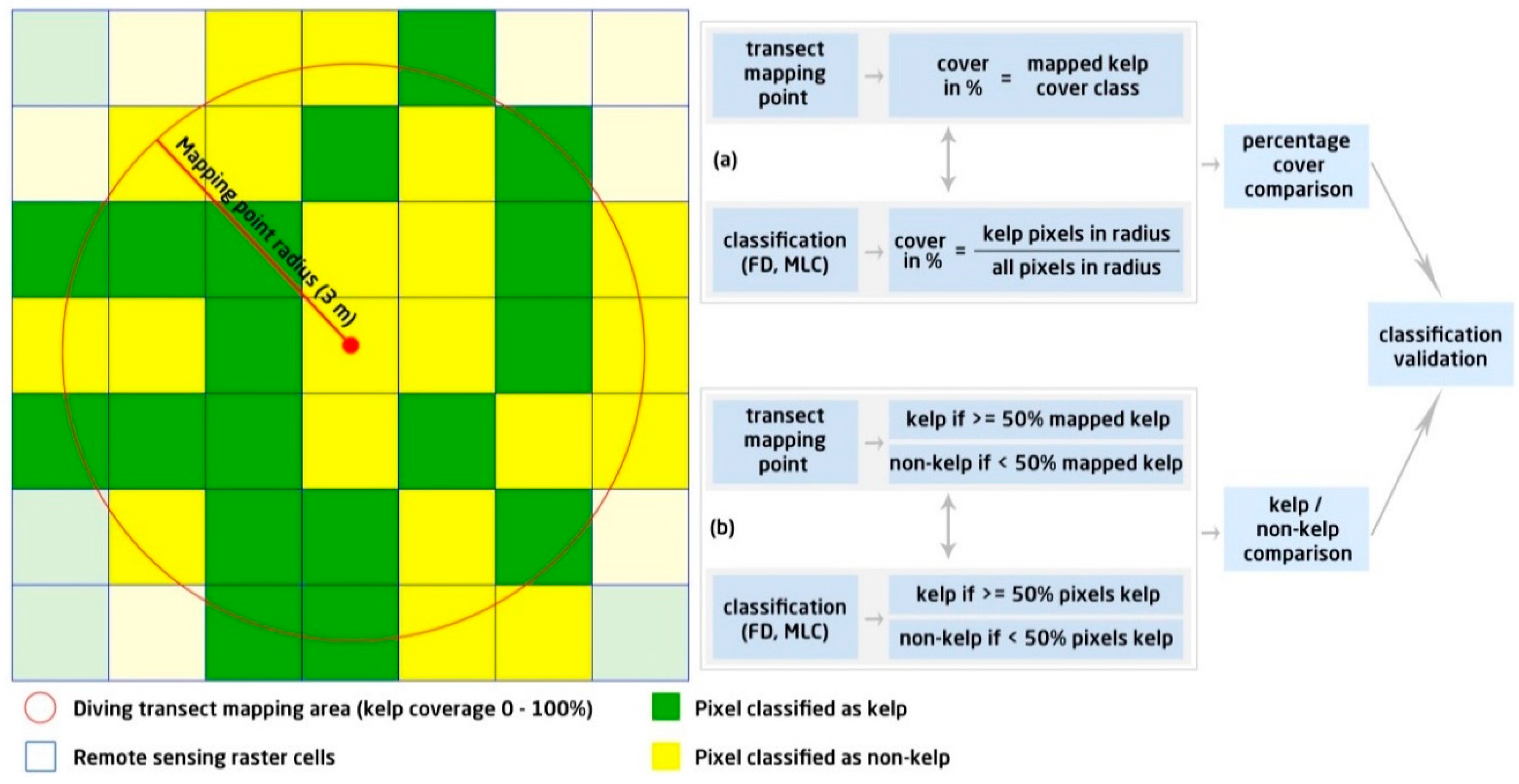
2.6. Validation of Classification Results

The spatial resolution of the AisaEAGLE data is higher than the transect mappings with an approximate radius of three metres around each mapping point (Figure 3); on average, 38 pixels cover the same area as a single diving mapping point. After FD and MLC classification, we adjusted the remote sensing data to the spatial resolution of the diving mapping and examined the accuracy of the classification results with two methods. For the first statistical analysis, we calculate the percentage cover from the AISA classifications by counting all kelp pixels and dividing them by the total number of pixels within the range of a mapping point. We then compare this measure to the mapped kelp cover for the respective transect mapping point (Figure 3a). This method is used to validate the results from each single flight stripe and to exclude unsuitable flight stripes from further analysis. For each flight stripe we calculate three accuracy measures, i.e., root-mean-square error (RMSE), Pearson product-moment correlation coefficient (R2) and Nash–Sutcliffe model efficiency coefficient (NSE) [77]. We use the setup of three different measures to confirm the accuracies with different accuracies: the RMSE is the average percentage deviation between the diving mapping and the kelp detection results; R2 is a measure for a linear correlation between both datasets and NSE assesses the overall match of mapped and remotely sensed data. NSE = 0 indicates an accuracy as good as the mean of the mapped data, values close to +1 refer to an accurate detection and negative values indicate that the accuracy is worse than the mean of the mapped data.
The second statistical analysis evaluates the feasibility of FD and MLC to distinguish kelp-dominated and non-kelp areas (Figure 3b). An area is marked as kelp dominated, if 50% or more of the pixels within the reach of a validation point detect kelp. We also adjust the diving transects mapping to this differentiation, i.e., a mapping point result indicating >50% coverage of brown algae is flagged as presence of kelp. Prior to the second analysis, a subset of suitable flight stripes determined by the first analysis is merged to single image. Accuracy measures are the overall accuracy, error of omission and error of commission [78].

3. Results and Discussion

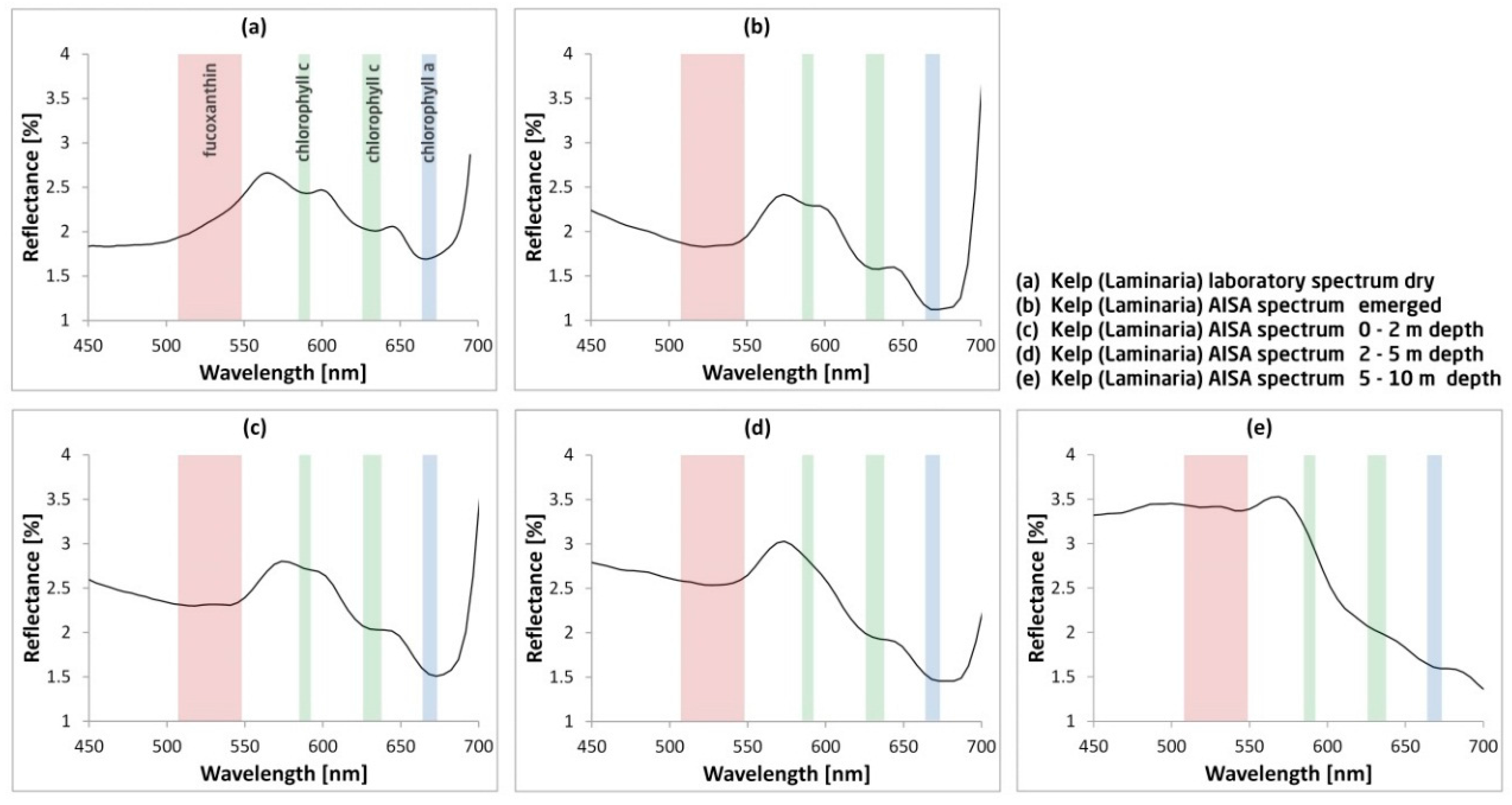
3.1. Wavelength Range for Deep Kelp Detection

The photochemical properties of kelp mainly influence the spectral reflectance in the visible part of the electromagnetic spectrum. For SAV, the spectral properties of water influence these spectral characteristics. The location of spectral features shifts with varying water level or features may even disappear. The behaviour of kelp spectra under varying water column is the basis to determine the wavelength intervals of the FD algorithm because the FD algorithm requires unique local reflectance minima or maxima. To determine suitable wavelength intervals, we extracted kelp spectra from the AisaEAGLE data at different depth levels. Figure 4 shows a sequence of AISA Laminaria spectra achieved from different depth positions (Figure 4b–e) derived from the bathymetric map depth classes in comparison to a dry kelp laboratory spectrum (Figure 4a) [38]. The characteristic absorption troughs of the main pigments fucoxanthin, chlorophyll c and chlorophyll a are highlighted for each spectrum. The absorption features from all pigments are visible in the laboratory spectrum (Figure 4a) as well as in the AISA spectrum (Figure 4b). A water depth of 0–2 m results in a less distinctive chlorophyll c absorption and the disappearance of spectral troughs at 585 nm and 630 nm (Figure 4c).
Increasing water depth also affects other spectral features (Figure 4d). A reflectance peak at 570 nm and troughs at 527 nm and 675 nm are the only local maxima/minima still detectable at 2–5 m. At a depth of 5–10 m (Figure 4e), the water absorbs electromagnetic radiation >680 nm; the chlorophyll absorption at 675 nm therefore becomes undetectable. Reflectance between 450 and 570 nm is higher compared to the shallower algae spectra due to additional reflection of the turbid waters. The spectral analysis reveals only two spectral features of kelp for all depth levels. The first is the wavelength range of 510–546 nm mainly influenced by fucoxanthin absorption, whereas this absorption feature shifts from shorter wavelengths (low water influence, Figure 4b) to longer wavelengths (deeper areas, Figure 4e). The second feature is a reflectance peak between 560 and 580 nm. The results clearly show that the wavelength region >600 nm is unsuitable to detect spectral features of submerged kelp. In the turbid waters around Helgoland, longer wavelengths are only feasible for the detection of shallow, emergent or floating algae. To detect kelp in different water depths, it is necessary to use the spectral range between 500 and 600 nm, where two suitable spectral features are located at 528 nm ± 18 nm and at 570 nm ±10 nm.

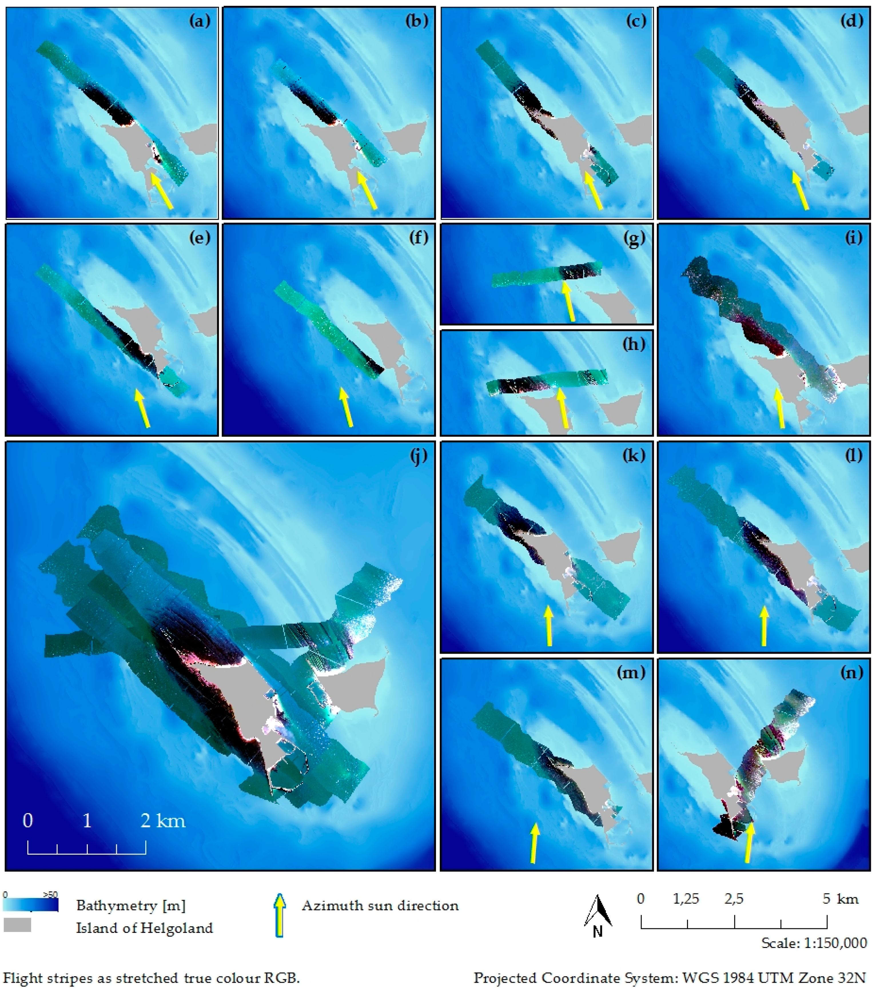
3.2. WAF Performance

Water anomalies have a strong influence on the results of the feature detection algorithm. Initial tests of feature detection without prior filtering resulted in erroneous kelp detection at sites influenced by sun glint. By removing outliers WAF significantly improves the FD results. Figure 5 shows some examples of WAF performance. The imagery is strongly influenced by sunglint before data correction (Figure 5a,c) while sun glint is significantly reduced by filtering (Figure 5b,d).
WAF performance may also be an indicator of data quality, because the amount of corrected pixels indicates image homogeneity. Table 2 shows the percentage of WAF corrected pixels for every flight stripe.
The data depict an increasing percentage of corrected pixels with increasing flight stripe. Moreover, the flight stripes eight and nine show exceptionally high numbers of corrected pixels. Visual analysis reveals an increase of sunglint from flight stripe one to flight stripe thirteen. The flight stripe numbers correspond with the time of day during image acquisition (Table 1), whereas azimuth flight direction remains constant for most of the stripes except 7, 8 and 13. Azimuth sun movement resulting in changing sun-sensor geometries is therefore the main reason for increasing sunglint. The flight parameters from stripes seven, eight and thirteen corroborate this hypothesis. The flight direction is approximately from west to east with sun coming from south, while the other data has been recorded in south-east to north-west flight direction. In these stripes, WAF is not able to sufficiently correct the sunglint-artefacts, because the glint covered areas are much larger than the filter kernel size of 5 × 5 pixels. For feature detection, non-filtered data performed poorly.

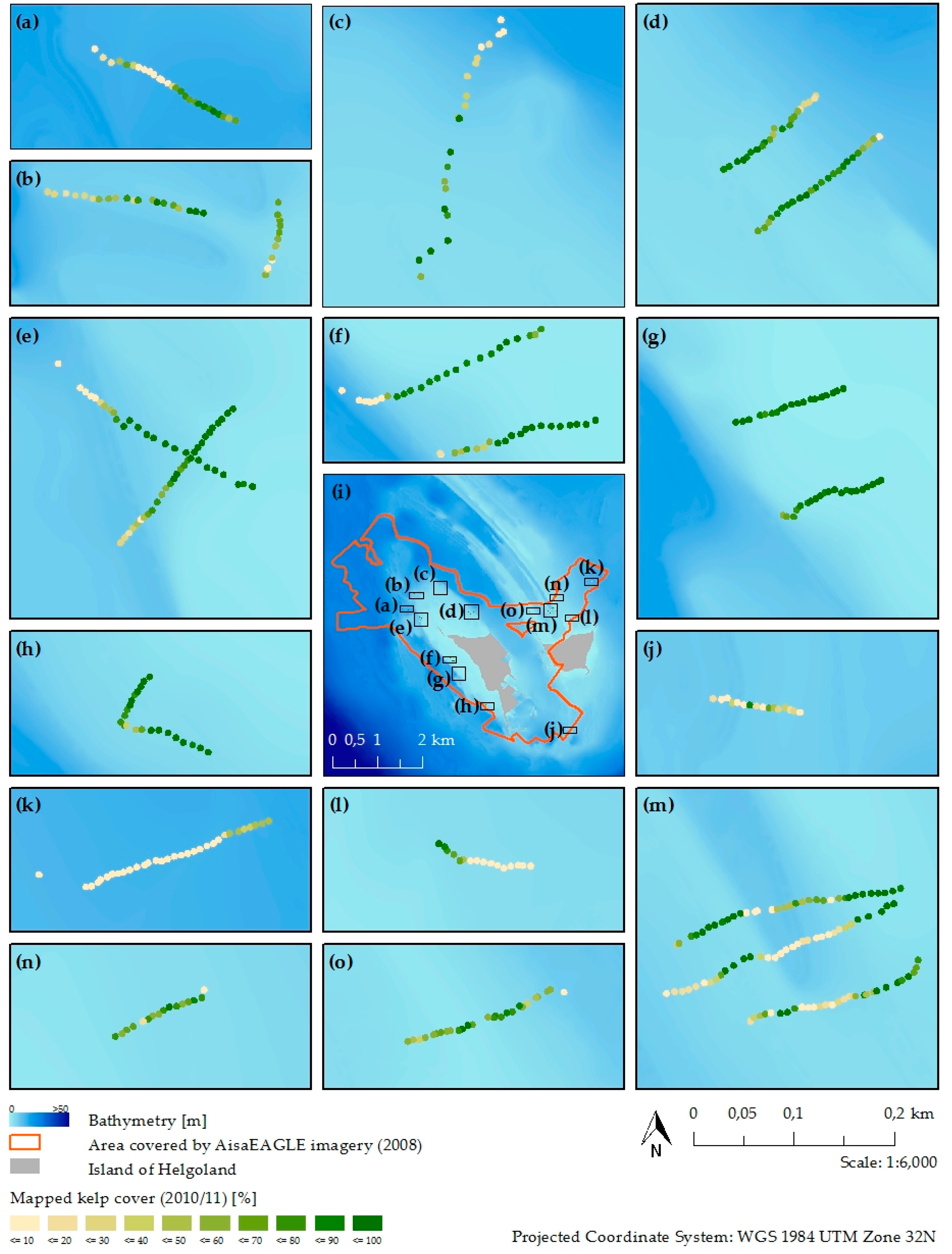
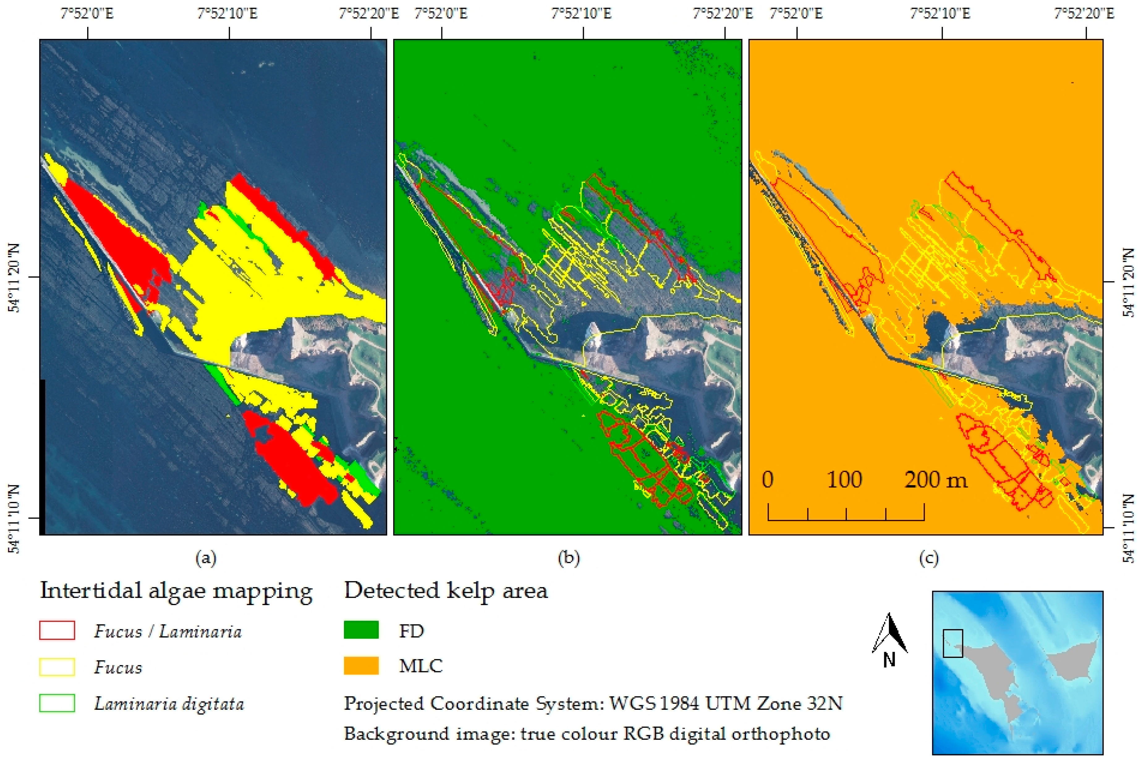
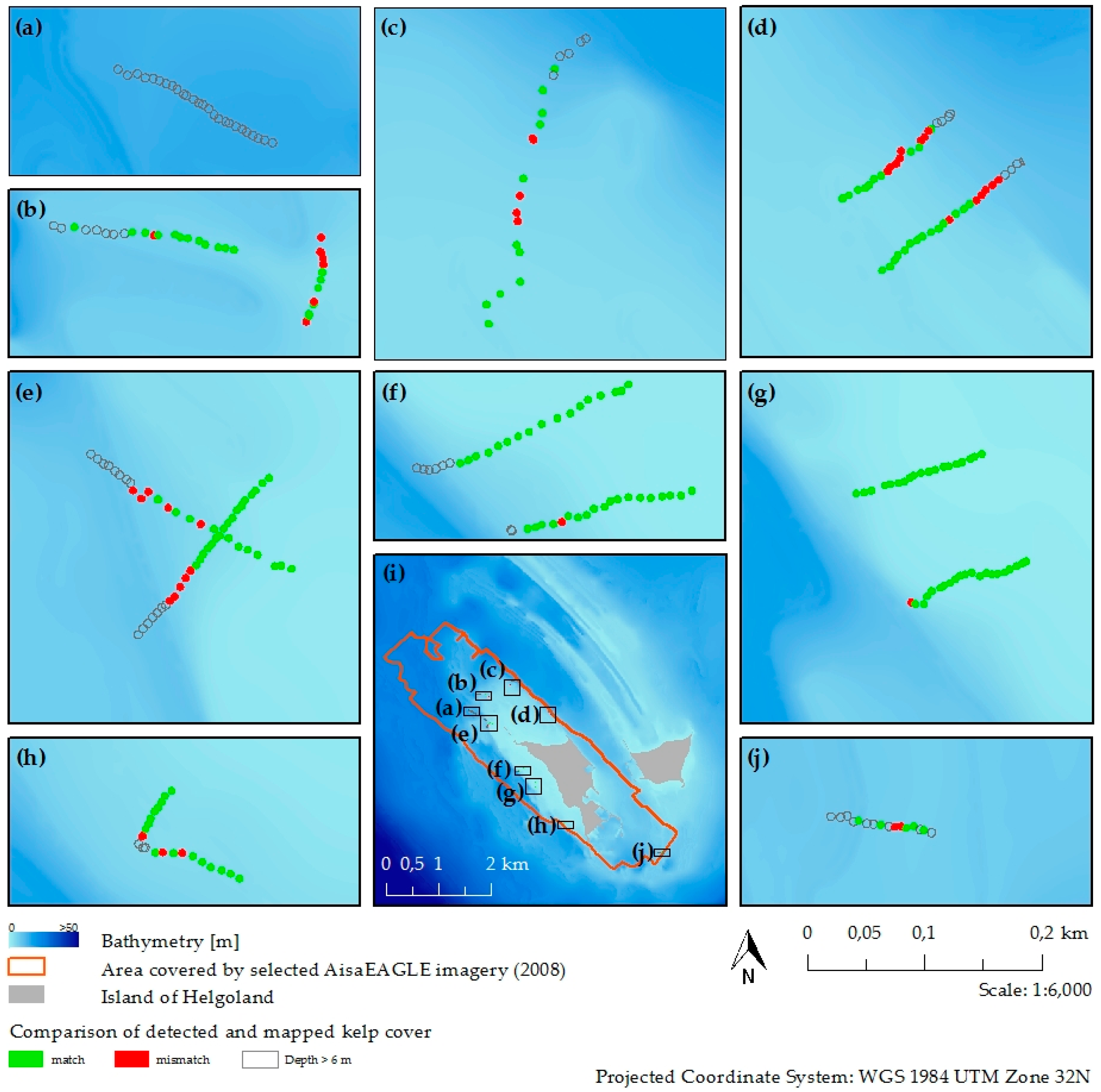
3.3. Kelp Detection Results Validated with Diving Transects

Interpreting kelp detection results visually, feature detection successfully captures the kelp forests in the deep waters around Helgoland. The approach identifies kelp on the rocky ridges and excludes sandy channels (Figure 6). Reflectance signal from the rocky bottom substrates did not influence the kelp detection results. Macroalgae completely cover the solid substrates in the intertidal. The reflected signal from these areas is therefore mainly influenced by the water column and macroalgae. Kelp does not grow on unconsolidated substrates. Spectral mixing between the sandy ridges and kelp is not a major problem for this study area. Only the small edges between the two habitats suffer from spectral mixing. Therefore, both covers could clearly be separated by the kelp detection.
Analysis of the diving data and the bathymetric map shows that the maximum depth for hyperspectral kelp detection around Helgoland is approximately six metres. Secchi depth measurements on 9 May 2008 from the Helgoland Reede time-series reveal 4.1 m visibility depth [79]. We assumed that the Secchi depth may be the limit for optical kelp detection; however, FD exceeds the expectations by two metres. This difference may be explained by the growth form of kelp, which stands semi-erect in the water column, whereas the bathymetric map gives the depth to the sea floor. Thus, the path of the light can be shorter to the canopy of the kelp than to the sea floor. The divers also mapped kelp deeper than six metres, but these areas are not detected by the feature detection in the study area. We therefore reduced the diving mapping data to the depth range of zero to six metres for classification validation (Figure 7). We first verified whether the feature detection successfully estimates percentage coverage of kelp. Table 3 shows the validation results for the FD using the diving data.
Validation with the transect mapping shows poor results, except flight stripe five and six which show RMSE lower than 20%, R2 greater or equal to 0.7 and NSE at approximately 0.6. Results from the percentage kelp cover estimation showed poor results, indicating that FD might not be suitable to measure kelp coverage. Nevertheless, the calculated low accuracies do not match the good visual interpretation results from Figure 6 and comparison with digital orthophotos and field photography showed good conformity with the FD results. We attribute the low accuracies to several factors. The low position accuracy of the diving transects (±25 m) is a substantial problem. The buoy GPS measurement induced an inaccuracy of several metres in the diving data as measurements were non-differentially corrected and there always was a misalignment between buoy and diver position, which tend to float and therefore constantly change their positions and field of view towards the measurement points. However, the AisaEAGLE data have a high spatial resolution of 1 × 1 m contrary to the spatial inaccuracy of the in situ measurements. This mismatch between imagery and ground truth data induces a failure in the correlation between percentage cover estimation by the divers and the hyperspectral imagery. The time-lag of two to three years between field mapping and remote sensing data acquisition may also have induced an error. Furthermore, classification errors primarily occur at pixels with insufficient sunglint removal. Conventional sunglint removal methods may be suitable to reduce the sunglint and thus also the classification errors [80,81,82]. However, a first attempt to correct the sunglint with the method introduced by Kutser et al., (2009) showed unsatisfactory results. This is mainly addressed to the differing waterbodies around Helgoland. Flight stripes seven, eight and thirteen were therefore excluded from further analysis. Strong movements of the aircraft during recording of flight stripe nine caused errors in the geometric correction, which results in highly inaccurate pixel locations (validated visually with digital orthophotos and other flight stripes). We therefore also excluded this stripe from further investigation.
The second statistical analysis evaluates the feasibility of the feature detection to distinguish kelp-dominated and non-kelp pixels. Therefore, we merged the results of the kelp detection from all remaining flight stripes to a single image (Figure 7i) and did not calculate accuracy measures for each single flight stripe.
We compared the results of the FD and mapping results achieving satisfactory accuracies. The overall accuracy of the kelp/non-kelp detection is 80.18%. 178 out of 222 pixels of the diving mapping match the remote sensing data. Of special interest are the classification errors: the error of omission is 18.92% indicating that FD was unable to identify approximately 20% of the kelp mapped by the divers; with 0.90% the error of commission indicates that detected kelp pixels are nearly always true kelp pixels. FD therefore is suitable for identifying absence or presence of kelp.

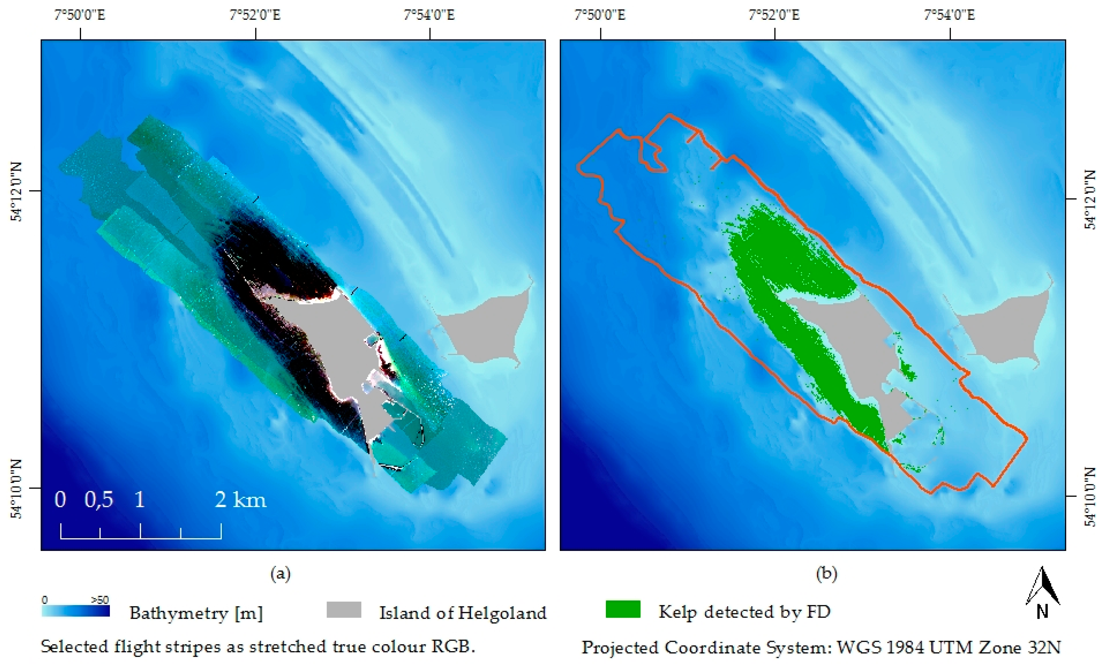
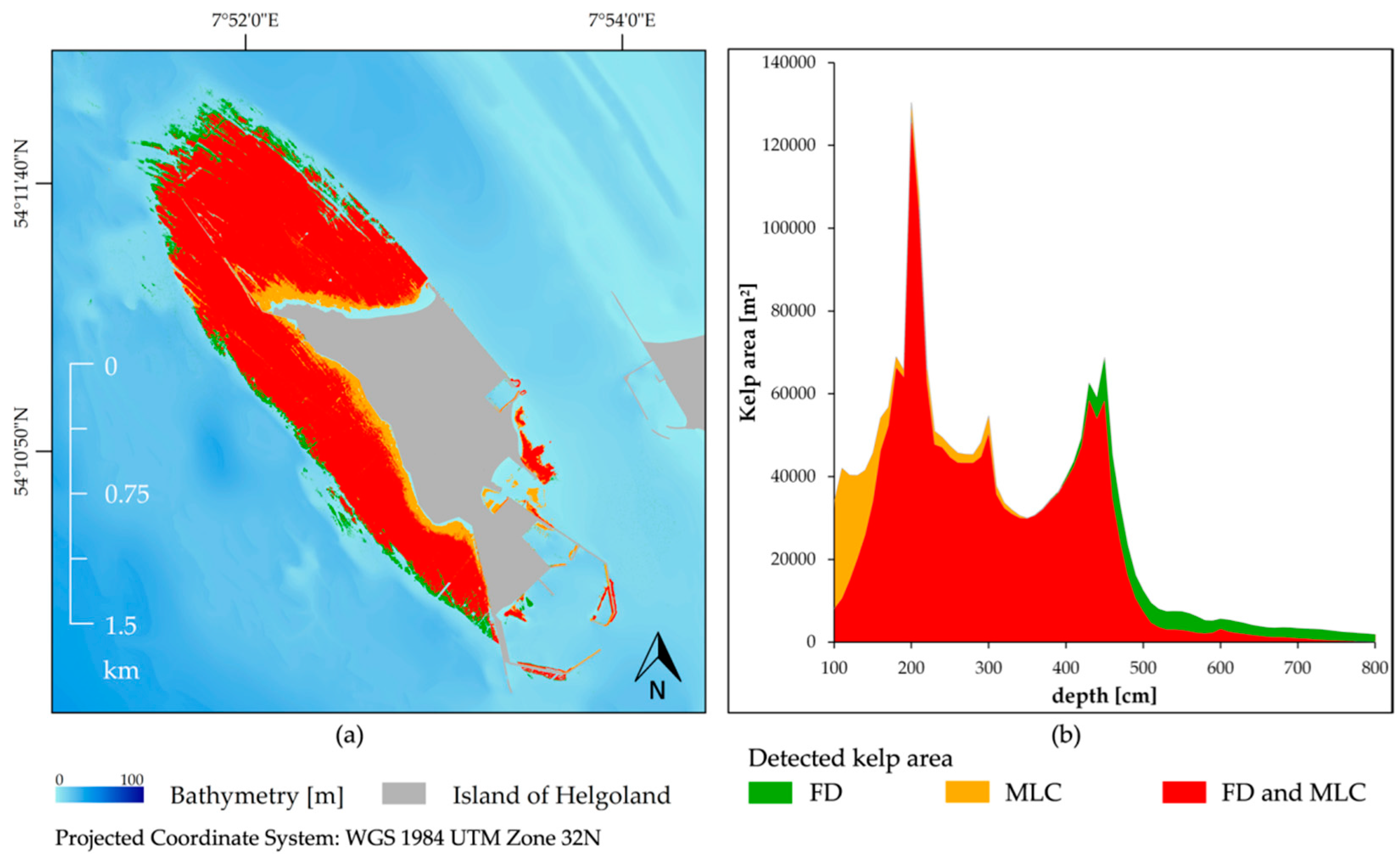
3.4. Feature Detection Results Validated with Maximum Likelihood Classifier

Spatial variations between the in situ data and the remote sensing data are one of the main reasons for lower accuracy measures of the kelp cover and presence/absence estimation. Therefore, in situ data alone seem to be insufficient to assess the suitability of the FD for kelp detection. We compared the FD to results with a commonly used MLC technique. This procedure enables an exact spatial comparability of the results. The flight stripes selected for this analysis capture the kelp forests around the main island and the area covered by them is shown in Figure 7i. We validated the MLC results comparable to the FD results (Section 3.3). Table 4 shows the accuracy measures of the MLC.
Compared to FD, MLC accuracies are significantly lower for all measures (RMSE Ø −13.42; R2 Ø −0.17; NSE Ø −1.46); except for flight stripes eleven and twelve. Nevertheless, the poor accuracies support the findings from Section 3.3, that georeferencing of diving mappings may be unsuitable to validate remote sensing data with high spatial resolution. For the second statistical measure, the kelp/non-kelp detection, we again merged the results of the MLC from the selected flight stripes to a single image. This analysis reveals an overall accuracy of 57.66% (n = 222), which is 22.52% lower than for the FD approach. The error of omission is 42.34% and the error of commission is zero. Thus, no areas have been falsely declared as kelp, but MLC was unable to identify several kelp areas (94 of 222 transect mapping points).
The total cover of kelp detected by FD is 1.90 km2 while MLC detects 1.93 km2. Although there is only a small difference in the total area of detected kelp between both classifications, detected areas are distributed unevenly. Figure 8a shows the spatial comparison of the two kelp detection results, visualizing that 80.45% of the kelp area matches for both methods, but MLC classifies 10.42% of kelp coverage mainly in very shallow waters close to the coastline, whereas FD detects 9.13% in waters deeper than 4 m. Table 5 shows the accuracies of FD and MLC for different depth limits using the diving depth gauge measures.
The overall accuracy of MLC drops significantly with a depth of four metres, while FD still sufficiently detects kelp at six metres depth (overall accuracy = 80.18). Figure 8b shows that the decreasing accuracy mainly results from kelp patches unidentified by MLC. The fully automatic FD detects kelp areas deeper than four metres with higher accuracy than the MLC. Both classifiers identify kelp between two and four metres water depth; due to the intensive training, however, MLC is much more labour-intensive. Nevertheless, differences between the two approaches are especially high in shallow waters (<2 m, Figure 8b). The diving mappings do not capture the transitional zones close to the intertidal habitats. Using digital orthophotos and intertidal mappings, we found MLC to falsely identify spectrally similar Fucales habitats as kelp (Figure 9c).
However, FD only identifies few Fucales habitats as kelp. Diving mappings do not reveal this error of commission of MLC and FD because species of the order Fucales do not grow in the intertidal areas mapped by the divers. Furthermore, FD clearly reveals the depth dependent transition from kelp to Fucales habitats (Figure 9, red polygons). The deeper areas of these mixed habitats are mainly dominated by kelp, shifting to Fucales dominated areas in the shallow waters close to the island. Using multiple algae classes and depth dependent training for the MLC should overcome the false classification but is related to even more intense field mappings and classifier training. Furthermore, a comparison of both methods is only given, if both techniques distinguish between the same classes. Our results show that detection of submerged kelp still remains a challenge. Nevertheless, there are several indices, also from open ocean applications, that have already shown successful to detect emergent kelp, e.g., FAI [83], MCI [84] or even the terrestrial NDVI. We expect that a combination of such an index with the FD algorithm may improve the performance for shallow habitats, for example to fully separate Fucales habitats from kelp habitats. Suitable in situ data, however, is still necessary to adjust and validate a combined approach.

4. Conclusions

The results clearly demonstrate the potential of FD to map sublittoral kelps as shown in this case study from Helgoland (North Sea). WAF is a promising filter to remove water anomalies from turbid coastal waters and furthermore allows for improving remote sensing data quality. The mismatch of spatial position accuracy of the hyperspectral imagery with the diving transects was insufficient to validate percentage coverage products of kelp from high spatial resolution remote sensing data. We therefore validated the FD algorithm with MLC classification results. FD is a suitable and time-effective approach to assess and monitor submerged kelp at the limit of water visibility depth in the turbid coastal waters of Helgoland. The fully automated simple processor depends on reflectance derivatives and identifies kelp using spectral features in the wavelength range of 500–600 nm. The width of the features is >20 nm; the approach might therefore be transferred easily to satellite borne sensors or other areas to detect deep kelp. Furthermore, the FD was able to separate Fucales habitats from kelp habitats in the shallow waters. MLC failed in distinguishing these two brown algae covers. The MLC training process is much more time consuming than the FD and the results strongly depend on the availability of training data. Furthermore, supervised classifiers rely on absolute reflectance data; the class statistics are calculated from the remote image, and transfer to other data requires repeated training. To improve the performance of the FD approach, a combination with algae indices (like FAI, MCI) [85] may be promising.

Acknowledgments

The airborne image acquisition and data processing was partly funded by the European Fond for Regional Development within the project “Flexihyp”. We gratefully acknowledge OHB Systems AG for providing the motor glider and pilot, Franziska Nehring and Frederic Tardek of FIELAX GmbH for processing the AISA data. We acknowledge the considerable effort of the divers Claudia Daniel, Gabriele Dederer and team, Philipp Schubert and the diving team of the Biologische Anstalt Helgoland to generate sublittoral ground truth data. The authors thank the anonymous reviewers for their valuable comments and suggestions to improve the quality of the paper.

Author Contributions

Florian Uhl analyzed the data; Florian Uhl and Natascha Oppelt conceived and designed the automated processor; Florian Uhl wrote the paper; Inka Bartsch contributed remote sensing and biological data; Inka Bartsch contributed biological analysis.

Conflicts of Interest

The authors declare no conflict of interest.

Abbreviations

The following abbreviations are used in this manuscript:
SAVSubmerged aquatic vegetation
FDFeature detection
FSFlight stripe
MLCMaximum likelihood classifier
FAIFloating algae index
MCIMaximum chlorophyll index
NDVINormalized differenced vegetation index
RMSERoot-mean-square error
R2Pearson product-moment correlation coefficient
NSENash–Sutcliffe model efficiency coefficient

Appendix

Figure A1. (a) Stretched true colour images of all flight stripes and azimuth sun direction during data acquisition (a) FS 1 (b) FS 2 (c) FS 3 (d) FS 4 (e) FS 5 (f) FS 6 (g) FS 7 (h) FS 8 (i) FS 9 (j) mosaic of all FS (k) FS 10 (l) FS 11 (m) FS 12 (n) FS 13.
Remotesensing 08 00487 g010

References

  1. Halpern, B.S.; Walbridge, S.; Selkoe, K.A.; Kappel, C.V.; Micheli, F.; D’Agrosa, C.; Bruno, J.F.; Casey, K.S.; Ebert, C.; Fox, H.E.; et al. A Global Map of Human Impact on Marine Ecosystems. Science 2008, 319, 948–952. [Google Scholar] [CrossRef] [PubMed]
  2. Wiencke, C.; Bischof, K. (Eds.) Seaweed Biology; Springer Berlin Heidelberg: Berlin, Heidelberg, 2012.
  3. Hafting, J.T.; Craigie, J.S.; Stengel, D.B.; Loureiro, R.R.; Buschmann, A.H.; Yarish, C.; Edwards, M.D.; Critchley, A.T.; Graham, M. Prospects and challenges for industrial production of seaweed bioactives. J. Phycol. 2015, 51, 821–837. [Google Scholar] [CrossRef] [PubMed]
  4. Levin, P.S. Small-scale recruitment variation in a temperate fish: The roles of macrophytes and food supply. Environ. Biol. Fishes 1994, 40, 271–281. [Google Scholar] [CrossRef]
  5. Holbrook, S.J.; Carr, M.H.; Schmitt, R.J.; Coyer, J.A. Effect of Giant Kelp on Local Abundance of Reef Fishes: The Importance of Ontogenetic Resource Requirements. Bull. Mar. Sci. 1990, 47, 104–114. [Google Scholar]
  6. Van Iersel, S.; Flammini, A. Algae-Based Biofuels: Applications and Co-Products. Available online: http://www.fao.org/docrep/012/i1704e/i1704e.pdf (accessed on 25 March 2016).
  7. Yue, H.; Sun, Y.; Jing, H.; Zeng, S.; Ouyang, H. The Analysis of Laminaria japonica Industry and International Trade Situation in China. In Proceedings of Selected Articles of 2013 World Agricultural Outlook Conference; Xu, S., Ed.; Springer: Heidelberg, Germany, 2014; pp. 39–51. [Google Scholar]
  8. Kerrison, P.D.; Stanley, M.S.; Edwards, M.D.; Black, K.D.; Hughes, A.D. The cultivation of European kelp for bioenergy: Site and species selection. Biomass Bioenergy 2015, 80, 229–242. [Google Scholar] [CrossRef]
  9. Lüning, K.; Dring, M.J. Continuous underwater light measurement near Helgoland (North Sea) and its significance for characteristic light limits in the sublittoral region. Helgoländer Wiss. Meeresunters. (Helgoländer Wissenschaftliche Meeresuntersuchungen) 1979, 32, 403–424. [Google Scholar] [CrossRef]
  10. Mann, K.H. Seaweeds: Their Productivity and Strategy for Growth: The role of large marine algae in coastal productivity is far more important than has been suspected. Science 1973, 182, 975–981. [Google Scholar] [CrossRef] [PubMed]
  11. Dean, T.A.; Jacobsen, F.R. Growth of juvenile Macrocystis pyrifera (Laminariales) in relation to environmental factors. Mar. Biol. 1984, 83, 301–311. [Google Scholar] [CrossRef]
  12. Lüning, K. Seaweeds: Their Environment, Biogeography, and Ecophysiology; Wiley: New York, NY, USA, 1990. [Google Scholar]
  13. Harley, C.D.G.; Randall Hughes, A.; Hultgren, K.M.; Miner, B.G.; Sorte, C.J.B.; Thornber, C.S.; Rodriguez, L.F.; Tomanek, L.; Williams, S.L. The impacts of climate change in coastal marine systems. Ecol. Lett. 2006, 9, 228–241. [Google Scholar] [CrossRef] [PubMed]
  14. Kirihara, S.; Nakamura, T.; Kon, N.; Fujita, D.; Notoya, M. Recent fluctuations in distribution and biomass of cold and warm temperature species of Laminarialean algae at Cape Ohma, northern Honshu, Japan. In Eighteenth International Seaweed Symposium; Anderson, R., Brodie, J., Onsøyen, E., Critchley, A.T., Eds.; Springer: Dordrecht, The Netherlands, 2007; pp. 295–301. [Google Scholar]
  15. Johnson, C.R.; Banks, S.C.; Barrett, N.S.; Cazassus, F.; Dunstan, P.K.; Edgar, G.J.; Frusher, S.D.; Gardner, C.; Haddon, M.; Helidoniotis, F.; et al. Climate change cascades: Shifts in oceanography, species’ ranges and subtidal marine community dynamics in eastern Tasmania. J. Exp. Mar. Biol. Ecol. 2011, 400, 17–32. [Google Scholar] [CrossRef]
  16. Bartsch, I.; Paar, M.; Fredriksen, S.; Schwanitz, M.; Daniel, C.; Hop, H.; Wiencke, C. Changes in kelp forest biomass and depth distribution in Kongsfjorden, Svalbard, between 1996–1998 and 2012–2014 reflect Arctic warming. Polar Biol. 2016. [Google Scholar] [CrossRef]
  17. Sogn Andersen, G.; Steen, H.; Christie, H.; Fredriksen, S.; Moy, F.E. Seasonal Patterns of Sporophyte Growth, Fertility, Fouling, and Mortality of Saccharina latissima in Skagerrak, Norway: Implications for Forest Recovery. J. Mar. Biol. 2011. [Google Scholar] [CrossRef]
  18. Díez, I.; Muguerza, N.; Santolaria, A.; Ganzedo, U.; Gorostiaga, J.M. Seaweed assemblage changes in the eastern Cantabrian Sea and their potential relationship to climate change. Estuar. Coast. Shelf Sci. 2012, 99, 108–120. [Google Scholar] [CrossRef]
  19. Wernberg, T.; Russell, B.D.; Thomsen, M.S.; Gurgel, C.F.D.; Bradshaw, C.J.; Poloczanska, E.S.; Connell, S.D. Seaweed Communities in Retreat from Ocean Warming. Curr. Biol. 2011, 21, 1828–1832. [Google Scholar] [CrossRef] [PubMed]
  20. Voerman, S.E.; Llera, E.; Rico, J.M. Climate driven changes in subtidal kelp forest communities in NW Spain. Mar. Environ. Res. 2013, 90, 119–127. [Google Scholar] [CrossRef] [PubMed]
  21. Müller, R.; Laepple, T.; Bartsch, I.; Wiencke, C. Impact of oceanic warming on the distribution of seaweeds in polar and cold-temperate waters. Bot. Mar. 2009, 52, 617–638. [Google Scholar] [CrossRef]
  22. Jueterbock, A.; Tyberghein, L.; Verbruggen, H.; Coyer, J.A.; Olsen, J.L.; Hoarau, G. Climate change impact on seaweed meadow distribution in the North Atlantic rocky intertidal. Ecol. Evol. 2013, 3, 1356–1373. [Google Scholar] [CrossRef] [PubMed] [Green Version]
  23. Krause-Jensen, D.; Duarte, C.M. Expansion of vegetated coastal ecosystems in the future Arctic. Front. Mar. Sci. 2014, 1. [Google Scholar] [CrossRef]
  24. European Parliament, Council of the European Union. Directive 2008/56/EC of the European Parliament and of the Council of 17 June 2008 establishing a framework for community action in the field of marine environmental policy (Marine Strategy Framework Directive). Off. J. Eur. Union 2008, 51, 19–40. [Google Scholar]
  25. Reichert, K.; Buchholz, F. Changes in the macrozoobenthos of the intertidal zone at Helgoland (German Bight, North Sea): A survey of 1984 repeated in 2002. Helgol. Mar. Res. 2006, 60, 213–223. [Google Scholar] [CrossRef] [Green Version]
  26. Merzouk, A.; Johnson, L.E. Kelp distribution in the northwest Atlantic Ocean under a changing climate. J. Exp. Mar. Biol. Ecol. 2011, 400, 90–98. [Google Scholar] [CrossRef]
  27. Van Rein, H.B.; Brown, C.J.; Quinn, R.; Breen, J. A review of sublittoral monitoring methods in temperate waters: A focus on scale. Underw. Technol. Int. J. Soc. Underw. Technol. 2009, 28, 99–113. [Google Scholar] [CrossRef]
  28. Zhang, X. On the estimation of biomass of submerged vegetation using Landsat thematic mapper (TM) imagery: A case study of the Honghu Lake, PR China. Int. J. Remote Sens. 1998, 19, 11–20. [Google Scholar] [CrossRef]
  29. Kutser, T.; Miller, I.; Jupp, D.L. Mapping coral reef benthic substrates using hyperspectral space-borne images and spectral libraries. Estuar. Coast. Shelf Sci. 2006, 70, 449–460. [Google Scholar] [CrossRef]
  30. Bertels, L.; Vanderstraete, T.; van Coillie, S.; Knaeps, E.; Sterckx, S.; Goossens, R.; Deronde, B. Mapping of coral reefs using hyperspectral CASI data; a case study: Fordata, Tanimbar, Indonesia. Int. J. Remote Sens. 2008, 29, 2359–2391. [Google Scholar] [CrossRef]
  31. Silva, T.S.F.; Costa, M.P.F.; Melack, J.M.; Novo Evlyn, M.L.M. Remote sensing of aquatic vegetation: Theory and applications. Environ. Monit. Assess. 2008, 140, 131–145. [Google Scholar] [CrossRef] [PubMed]
  32. Dekker, A.G.; Brando, V.E.; Anstee, J.M.; Pinnel, N.; Kutser, T.; Hoogenboom, E.J.; Peters, S.; Pasterkamp, R.; Vos, R.; Olbert, C.; et al. Imaging Spectrometry of Water. In Imaging Spectrometry: Basic Principles and Prospective Applications; van der Meer, F.D., Jong, S.M.D., Eds.; Kluwer Academic Publishers: Dordrecht, The Netherland, 2011; Volume 4, pp. 307–359. [Google Scholar]
  33. Simms, É.; Dubois, J.-M.M. Satellite remote sensing of submerged kelp beds on the Atlantic coast of Canada. Int. J. Remote Sens. 2001, 22, 2083–2094. [Google Scholar] [CrossRef]
  34. Vahtmäe, E.; Kutser, T. Mapping Bottom Type and Water Depth in Shallow Coastal Waters with Satellite Remote Sensing. J. Coast. Res. 2007, 50, 185–189. [Google Scholar]
  35. Fyfe, S.K. Spatial and temporal variation in spectral reflectance: Are seagrass species spectrally distinct? Limnol. Oceanogr. 2003, 48, 464–479. [Google Scholar] [CrossRef]
  36. Pinnel, N.; Heege, T.; Zimmermann, S. Spectral Discrimination of Submerged Macrophytes in Lakes Using Hyperspectral Remote Sensing Data. SPIE Proc. Ocean Opt. XVII 2004, 1, 1–16. [Google Scholar]
  37. Han, L.; Rundquist, D.C. The spectral responses of Ceratophyllum demersum at varying depths in an experimental tank. Int. J. Remote Sens. 2003, 24, 859–864. [Google Scholar] [CrossRef]
  38. Uhl, F.; Oppelt, N.; Bartsch, I. Spectral mixture of intertidal marine macroalgae around the island of Helgoland (Germany, North Sea). Aquat. Bot. 2013, 111, 112–124. [Google Scholar] [CrossRef]
  39. Malthus, T.J.; George, D.G. Airborne remote sensing of macrophytes in Cefni Reservoir, Anglesey, UK. Aquat. Bot. 1997, 58, 317–332. [Google Scholar] [CrossRef]
  40. Gitelson, A. The peak near 700 nm on radiance spectra of algae and water: Relationships of its magnitude and position with chlorophyll concentration. Int. J. Remote Sens. 1992, 13, 3367–3373. [Google Scholar] [CrossRef]
  41. Oppelt, N.; Schulze, F.; Bartsch, I.; Doernhoefer, K.; Eisenhardt, I. Hyperspectral classification approaches for intertidal macroalgae habitat mapping: A case study in Heligoland. Opt. Eng. 2012, 51. [Google Scholar] [CrossRef]
  42. Kutser, T.; Vahtmäe, E.; Martin, G. Assessing suitability of multispectral satellites for mapping benthic macroalgal cover in turbid coastal waters by means of model simulations. Estuar. Coast. Shelf Sci. 2006, 67, 521–529. [Google Scholar] [CrossRef]
  43. Roessler, S.; Wolf, P.; Schneider, T.; Melzer, A. Multispectral Remote Sensing of Invasive Aquatic Plants Using RapidEye. In Earth Observation of Global Changes (EOGC); [EOGC2011—3rd Earth Observation and Global Changes Conference, which was organized by Technische Universität München (TUM) in Germany, Peking University (China), and University of Waterloo (Canada)]; Krisp, J.M., Ed.; Springer: Berlin, Germany, 2013; pp. 109–123. [Google Scholar]
  44. Roelfsema, C.M.; Lyons, M.; Kovacs, E.M.; Maxwell, P.; Saunders, M.I.; Samper-Villarreal, J.; Phinn, S.R. Multi-temporal mapping of seagrass cover, species and biomass: A semi-automated object based image analysis approach. Remote Sens. Environ. 2014, 150, 172–187. [Google Scholar] [CrossRef]
  45. Hedley, J.; Roelfsema, C.; Chollett, I.; Harborne, A.; Heron, S.; Weeks, S.; Skirving, W.; Strong, A.; Eakin, C.; Christensen, T.; et al. Remote sensing of coral reefs for monitoring and management: A review. Remote Sens. 2016. [Google Scholar] [CrossRef]
  46. Kaufmann, H.; Segl, K.; Chabrillat, S.; Hofer, S.; Stuffler, T.; Mueller, A.; Richter, R.; Schreier, G.; Haydn, R.; Bach, H. EnMAP A Hyperspectral Sensor for Environmental Mapping and Analysis. In Proceedings of the 2006 IEEE International Symposium on Geoscience and Remote Sensing, Denver, CO, USA, 31 July–4 August 2006; pp. 1617–1619.
  47. Galeazzi, C.; Sacchetti, A.; Cisbani, A.; Babini, G. The PRISMA Program. In Proceedings of the IGARSS 2008—2008 IEEE International Geoscience and Remote Sensing Symposium, Boston, MA, USA, 7–11 July 2008; pp. 105–108.
  48. Schmidt, K.S.; Skidmore, A.K. Spectral discrimination of vegetation types in a coastal wetland. Remote Sens. Environ. 2003, 85, 92–108. [Google Scholar] [CrossRef]
  49. Phinn, S.; Roelfsema, C.; Dekker, A.; Brando, V.; Anstee, J. Mapping seagrass species, cover and biomass in shallow waters: An assessment of satellite multi-spectral and airborne hyper-spectral imaging systems in Moreton Bay (Australia). Remote Sens. Environ. 2008, 112, 3413–3425. [Google Scholar] [CrossRef]
  50. Dierssen, H.M.; Chlus, A.; Russell, B. Hyperspectral discrimination of floating mats of seagrass wrack and the macroalgae Sargassum in coastal waters of Greater Florida Bay using airborne remote sensing. Remote Sens. Environ. 2015, 167, 247–258. [Google Scholar] [CrossRef]
  51. Kluijver, M.J. Sublittoral hard substrate communities off Helgoland. Helgol. Meeresunters 1991, 45, 317–344. [Google Scholar] [CrossRef]
  52. Beermann, J.; Franke, H.-D. A supplement to the amphipod (Crustacea) species inventory of Helgoland (German Bight, North Sea): Indication of rapid recent change. Mar. Biodivers. Rec. 2011, 4. [Google Scholar] [CrossRef]
  53. DWD Climate Data Center (CDC). Downloadarchiv der Monats—Und Tageswerte von 78 Messstationen in Deutschland; Deutscher Wetterdienst: Offenbach, Germany, 2016. [Google Scholar]
  54. Franke, H.-D.; Gutow, L. Long-term changes in the macrozoobenthos around the rocky island of Helgoland (German Bight, North Sea). Helgol. Mar. Res. 2004, 58, 303–310. [Google Scholar] [CrossRef] [Green Version]
  55. Janke, K. Lebensgemeinschaften und ihre Besiedlungsstrukturen in der Gezeitenzone felsiger Meeresküsten: Die Bedeutung Biologischer Wechselwirkungen für die Entstehung und Erhaltung der Biozönose im Nordost-Felswatt von Helgoland; Dissertation: Kiel, Germany, 1989. [Google Scholar]
  56. Pehlke, C.; Bartsch, I. Changes in depth distribution and biomass of sublittoral seaweeds at Helgoland (North Sea) between 1970 and 2005. Clim. Res. 2008, 37, 135–147. [Google Scholar] [CrossRef]
  57. Bartsch, I.; Kuhlenkamp, R. The marine macroalgae of Helgoland (North Sea): An annotated list of records between 1845 and 1999. Helgol. Mar. Res. 2000, 54, 160–189. [Google Scholar] [CrossRef]
  58. Lüning, K. Tauchuntersuchungen zur Vertikalverteilung der sublitoralen Helgoländer Algenvegetation; Biologische Anstalt Helgoland: List auf Sylt, Germany, 1970. [Google Scholar]
  59. Bartsch, I.; Tittley, I. The rocky intertidal biotopes of Helgoland: Present and past. Helgol. Mar. Res. 2004, 58, 289–302. [Google Scholar] [CrossRef] [Green Version]
  60. Wasser- und Schifffahrtsverwaltung des Bundes (WSV) im Geschäftsbereich des Bundesministeriums für Verkehr und Digitale Infrastruktur. Available online: https://www.pegelonline.wsv.de/gast/start (accessed on 10 October 2015).
  61. Uhl, F.; Oppelt, N.; Bartsch, I. Mapping marine macroalgae in case 2 waters using CHRIS PROBA. In Proceedings of the ESA Living Planet Symposium, ESA Special Proceedings SP-722 (CD-ROM), Edinburgh, UK, 9–13 September 2013; p. CD-ROM.
  62. SPECIM Images. Aisa EAGLE Hyperspectral Sensor. Available online: http://cdn.metricmarketing.ca/www.spectralcameras.com/files/AISA/AisaEAGLE_datasheet_ver1–2013.pdf?this=that (accessed on 11 January 2016).
  63. Oxford Technical Solutions Limited. RTv2 GNSS-Aided Inertial Measurement Systems; Oxford Technical Solutions Limited: Oxford, UK, 2015. [Google Scholar]
  64. Richter, R.; Schlaepfer, D. Status of Model ATCOR4 on Atmospheric Topographic Correction for Airborne Hyperspectral Imagery, 2003. Available online: http://www.earsel.org/workshops/imaging-spectroscopy-2003/papers/data_enhancement/richter.pdf (accessed on 11 September 2013).
  65. Tec5 AG. HandySpec Field: A Portable Spectrometer System. In Proceedings of the 3rd EARSeL Workshop on Imaging Spectroscopy, Herrsching, Germany, 13–16 May 2003.
  66. Van der Linden, S.; Rabe, A.; Held, M.; Jakimow, B.; Leitão, P.; Okujeni, A.; Schwieder, M.; Suess, S.; Hostert, P. The EnMAP-Box—A Toolbox and Application Programming Interface for EnMAP Data Processing. Remote Sens. 2015, 7, 11249–11266. [Google Scholar] [CrossRef]
  67. Uhl, F.; Oppelt, N.; Bartsch, I. Einfaches Verfahren zur Bestimmung von marinen Algengemeinschaften mit Hilfe von hyperspektraler Fernerkundung. In Geoinformationen für die Küstenzone, Band 4: Beiträge des 4. Hamburger Symposiums zur Küstenzone und Beiträge des 9. Workshops zur Nutzung der Fernerkundung im Bereich der Bundesanstalt für Gewässerkunde/Wasser- und Schifffahrtsverwaltung des Bundes, 1st ed.; Traub, K.-P., Kohlus, J., Lüllwitz, T., Eds.; Sokrates & Freunde: Koblenz, Germany, 2013; pp. 233–245. [Google Scholar]
  68. Butler, W.L.; Hopkins, D.W. Higher derivative analysis of complex absorption spectra. Photochem. Photobiol. 1970, 12, 439–450. [Google Scholar] [CrossRef]
  69. Demetriades-Shah, T.H.; Steven, M.D.; Clark, J.A. High resolution derivative spectra in remote sensing. Remote Sens. Environ. 1990, 33, 55–64. [Google Scholar] [CrossRef]
  70. Tsai, F.; Philpot, W. Derivative Analysis of Hyperspectral Data. Remote Sens. Environ. 1998, 66, 41–51. [Google Scholar] [CrossRef]
  71. Savitzky, A.; Golay, M.J.E. Smoothing and Differentiation of Data by Simplified Least Squares Procedures. Anal. Chem. 1964, 36, 1627–1639. [Google Scholar] [CrossRef]
  72. Noiraksar, T.; Sawayama, S.; Phauk, S.; Komatsu, T. Mapping Sargassum beds off the coast of Chon Buri Province, Thailand, using ALOS AVNIR-2 satellite imagery. Bot. Mar. 2014, 57, 367–377. [Google Scholar] [CrossRef]
  73. Hoang, T.C.; O’Leary, M.J.; Fotedar, R.K. Remote-Sensed Mapping of Sargassum spp. Distribution around Rottnest Island, Western Australia, Using High-Spatial Resolution WorldView-2 Satellite Data. J. Coast. Res. 2015. [Google Scholar] [CrossRef]
  74. Lillesand, T.M.; Kiefer, R.W.; Chipman, J.W. Remote Sensing and Image Interpretation, 6th ed.; Wiley: Hoboken, NJ, USA, 2008. [Google Scholar]
  75. Pasqualini, V.; Pergent-MARTINI, C.; Fernandez, C.; Pergent, G. The use of airborne remote sensing for benthic cartography: Advantages and reliability. Int. J. Remote Sens. 1997, 18, 1167–1177. [Google Scholar] [CrossRef]
  76. Sawayama, S.; Nurdin, N.; Akbar, A.S.M.; Sakamoto, S.X.; Komatsu, T. Introduction of geospatial perspective to the ecology of fish-habitat relationships in Indonesian coral reefs: A remote sensing approach. Ocean Sci. J. 2015, 50, 343–352. [Google Scholar] [CrossRef]
  77. Nash, J.E.; Sutcliffe, J.V. River flow forecasting through conceptual models part I—A discussion of principles. J. Hydrol. 1970, 10, 282–290. [Google Scholar] [CrossRef]
  78. Campbell, J.B.; Wynne, R.H. Introduction to Remote Sensing, 5th ed.; Guilford Press: New York, NY, USA, 2011. [Google Scholar]
  79. Wiltshire, K.H.; Malzahn, A.M.; Wirtz, K.; Greve, W.; Janisch, S.; Mangelsdorf, P.; Manly, B.F.J.; Boersma, M. Resilience of North Sea phytoplankton spring bloom dynamics: An analysis of long-term data at Helgoland Roads. Limnol. Oceangr. 2008, 53, 1294–1302. [Google Scholar] [CrossRef]
  80. Hochberg, E.J.; Andrefouet, S.; Tyler, M.R. Sea surface correction of high spatial resolution ikonos images to improve bottom mapping in near-shore environments. IEEE Trans. Geosci. Remote Sens. 2003, 41, 1724–1729. [Google Scholar] [CrossRef]
  81. Hedley, J.D.; Harborne, A.R.; Mumby, P.J. Technical note: Simple and robust removal of sun glint for mapping shallow-water benthos. Int. J. Remote Sens. 2005, 26, 2107–2112. [Google Scholar] [CrossRef]
  82. Kutser, T.; Vahtmäe, E.; Praks, J. A sun glint correction method for hyperspectral imagery containing areas with non-negligible water leaving NIR signal. Remote Sens. Environ. 2009, 113, 2267–2274. [Google Scholar] [CrossRef]
  83. Hu, C. A novel ocean color index to detect floating algae in the global oceans. Remote Sens. Environ. 2009, 113, 2118–2129. [Google Scholar] [CrossRef]
  84. Gower, J.; King, S.; Borstad, G.; Brown, L. Detection of intense plankton blooms using the 709 nm band of the MERIS imaging spectrometer. Int. J. Remote Sens. 2005, 26, 2005–2012. [Google Scholar] [CrossRef]
  85. Hu, C.; Feng, L.; Hardy, R.F.; Hochberg, E.J. Spectral and spatial requirements of remote measurements of pelagic Sargassum macroalgae. Remote Sens. Environ. 2015, 167, 229–246. [Google Scholar] [CrossRef]
Figure 1. (a) The location of Helgoland is outlined in a map of Europe (data source: openstreetmapdata.com); (b) A bathymetric map based on sea chart level zero (lowest astronomical tide) of the subtidal zone of the archipelago (data source: courtesy of Federal Maritime and Hydrographic Agency of Germany 2010).
Remotesensing 08 00487 g001
Figure 2. Overview of diving transects (ah), flight stripe cover of the study area (i) and overview of diving transects (jo); the colouring indicates the percentage cover of kelp mapped by the divers.
Remotesensing 08 00487 g002
Figure 3. Validation of the Feature Detection (FD) and Maximum Likelihood Classification (MLC) results using a single diving transect mapping point: (a) percentage coverage comparison and (b) kelp/non-kelp detection.
Remotesensing 08 00487 g003
Figure 4. Savitzky-Golay smoothed kelp (Laminaria digitata) laboratory measurements (a) and Savitzky-Golay ROI AISA kelp (Laminaria hyperborea) spectra with varying water cover (be).
Remotesensing 08 00487 g004
Figure 5. Influence of water anomaly filtering (WAF performance) on imagery quality at sites influenced by sun glint. True colour RGB (639 nm/550 nm/459 nm) for two example areas. Area 1 before filtering (a) and after filtering (b) and area 2 before filtering (c) and after filtering (d).
Remotesensing 08 00487 g005
Figure 6. (a) Stretched true colour image of selected flight stripes and (b) kelp detected by FD.
Remotesensing 08 00487 g006
Figure 7. Kelp detection validation results with diving transect mapping (ah), cover of the selected flight stripes (i) and kelp detection validation results (j).
Remotesensing 08 00487 g007
Figure 8. Comparison of FD and MLC kelp detection results. (a) Spatial distribution of the classified kelp and (b) kelp area detected per depth.
Remotesensing 08 00487 g008
Figure 9. Intertidal field mappings compared to MLC and FD kelp detection results. Intertidal field mapping results (a); field mapping compared to FD results (b); field mapping compared to MLC results (c).
Remotesensing 08 00487 g009
Table 1. Flight stripe (FS) acquisition time of day (UTC).
FS12345678910111213
Start time10:0810:2010:2710:3410:4110:4810:5310:5911:0511:1911:2711:3611:42
Table 2. Pixels changed by the WAF in percent (%) of all pixels
Flight Stripe12345678910111213
corrected pixels (%)2.913.892.242.113.064.1511.6511.885.514.424.174.926.56
Table 3. Validation of the FD kelp detection results with dive transect mappings per flight stripe (FS).
FS12345678910111213
RMSE40.4542.6136.2841.2717.6518.5446.8545.2769.8359.1162.5857.3257.14
R20.430.430.400.380.700.720.390.330.060.160.200.290.03
NSE−1.42−1.28−1.02−0.930.570.65−0.81−0.94−4.90−2.05−2.29−1.93−1.25
Table 4. Validation of MLC results with dive transect mappings per flight stripe (FS).
FS123456101112
RMSE66.2045.5048.6262.0449.0457.6260.2259.4447.90
R20.120.390.190.200.270.250.130.210.39
NSE−5.44−1.59−2.61−3.33−2.33−2.37−2.16−1.95−1.03
Table 5. Depth dependent kelp/Non-kelp detection accuracies.
Depth Limit (m)123456
MLC overall accuracy (%)10092.6580.5365.6658.557.66
FD overall accuracy (%)10098.5396.4687.958280.18

