
Detecting Different Types of Directional Land Cover Changes Using MODIS NDVI Time Series Dataset


Abstract
:
1. Introduction
2. Materials and Methods
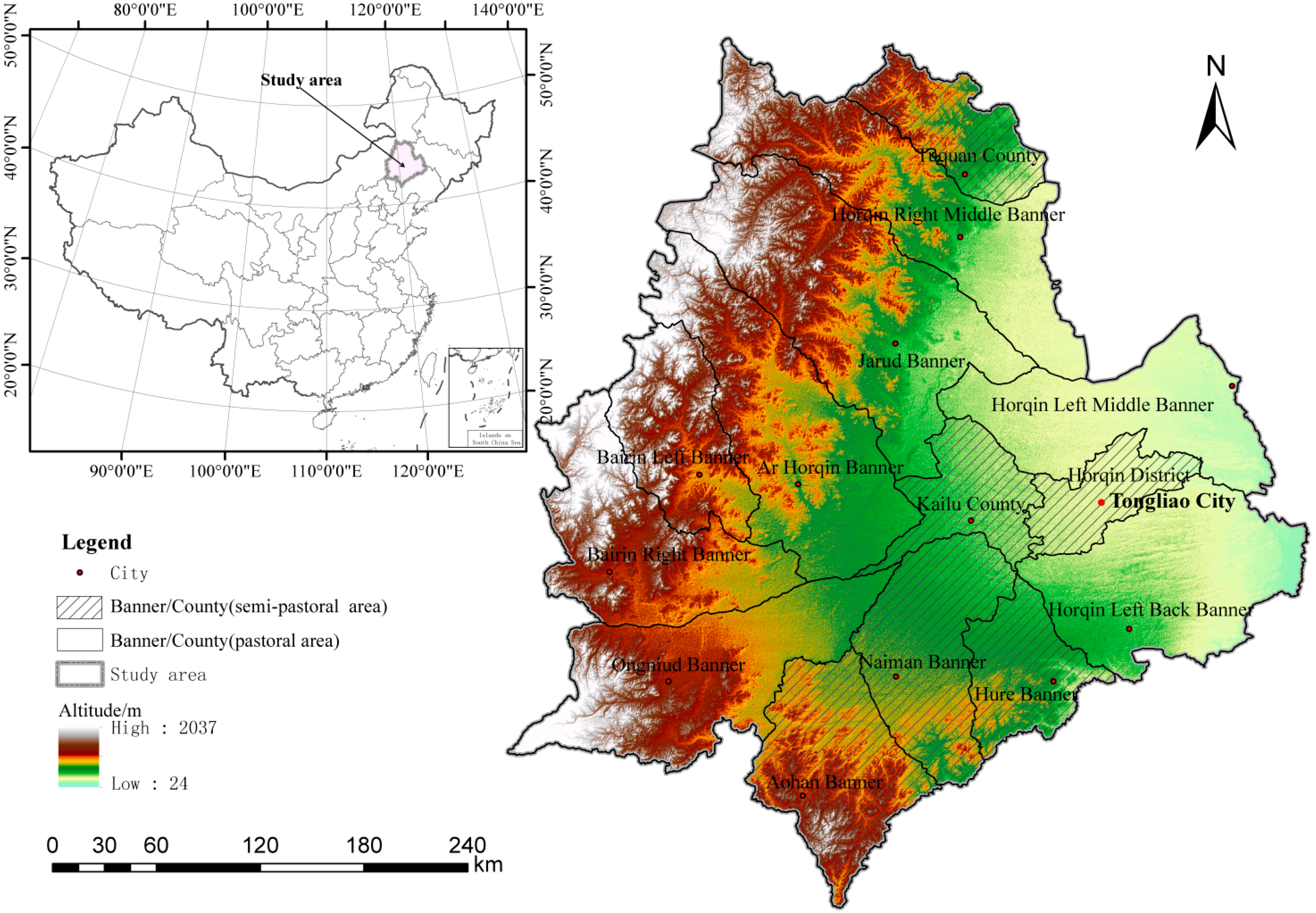
2.1. Study Area
2.2. Data and Data Preprocessing
2.3. Methodology
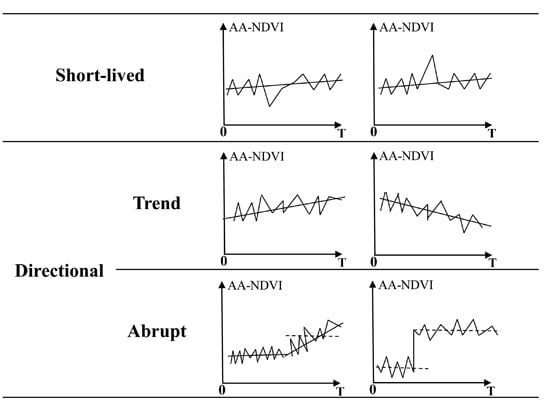
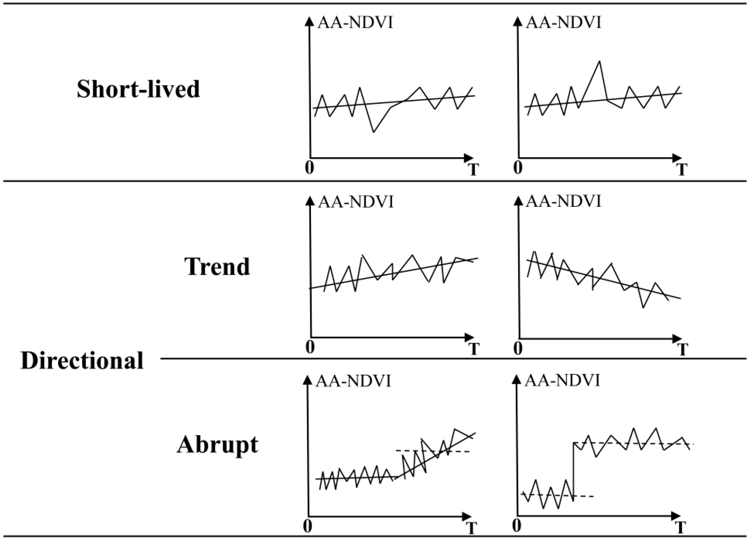
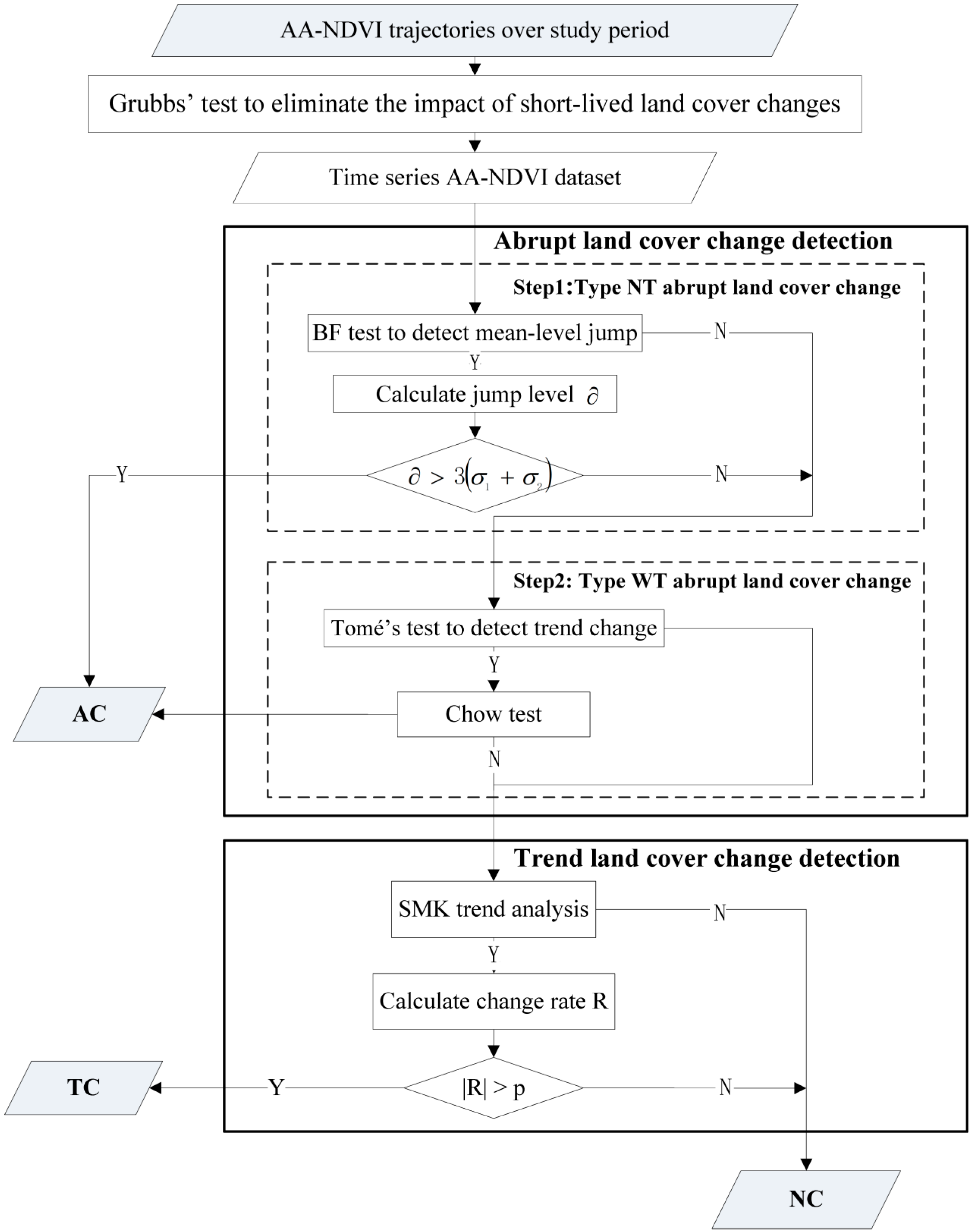
2.3.1. General Idea of the Method
2.3.2. Eliminating the Impact of Short-Lived Land Cover Changes
2.3.3. Abrupt Land Cover Change Detection
- (1)
- Type NT Abrupt Land Cover Change Detection
- (2)
- Type WT Abrupt Land Cover Change Detection
2.3.4. Trend Land Cover Change Detection
2.4. Technique Validation
2.4.1. Accuracies of Abrupt Land Cover Changes
2.4.2. Accuracies of Trend Land Cover Changes
3. Results
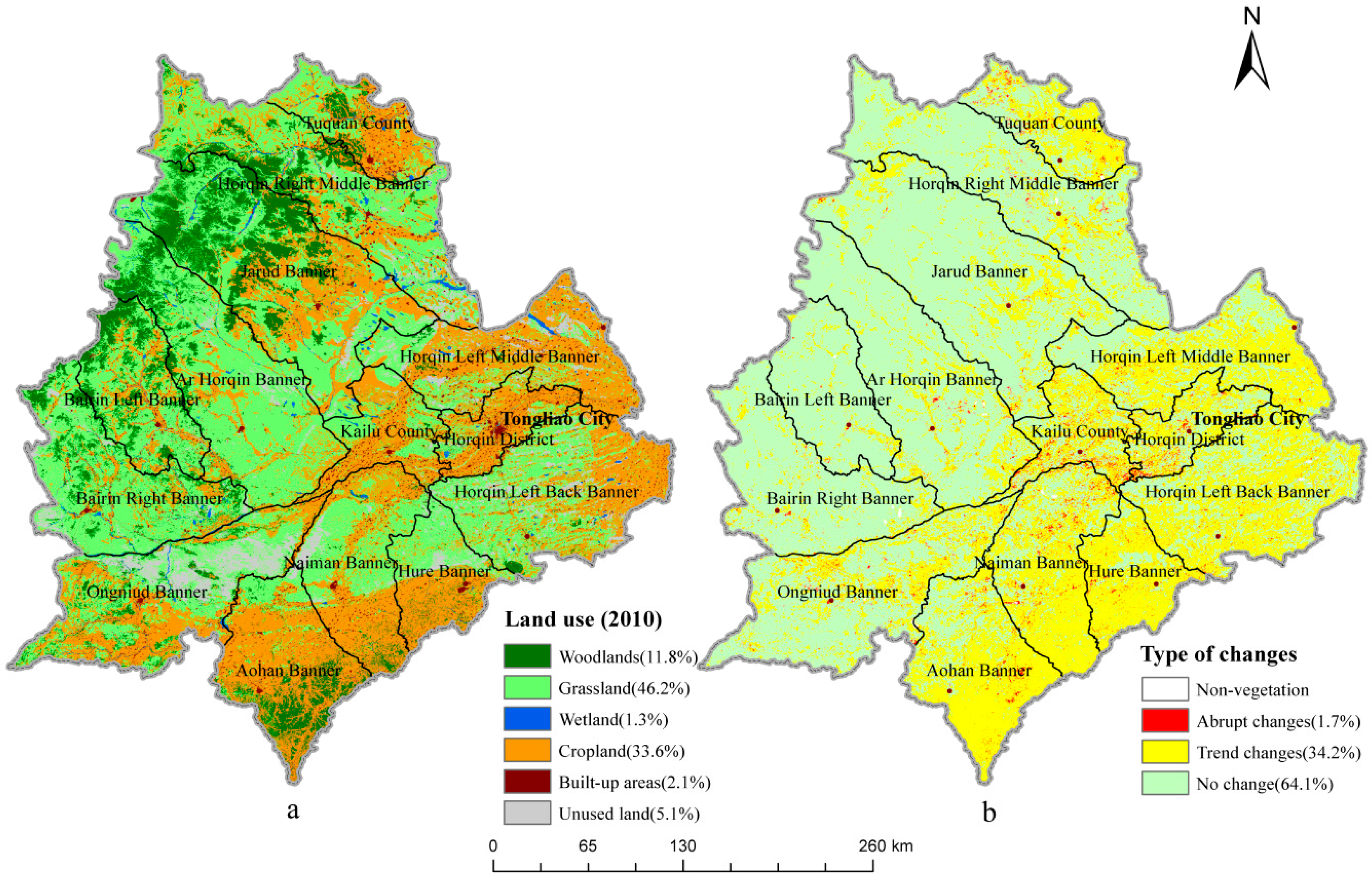
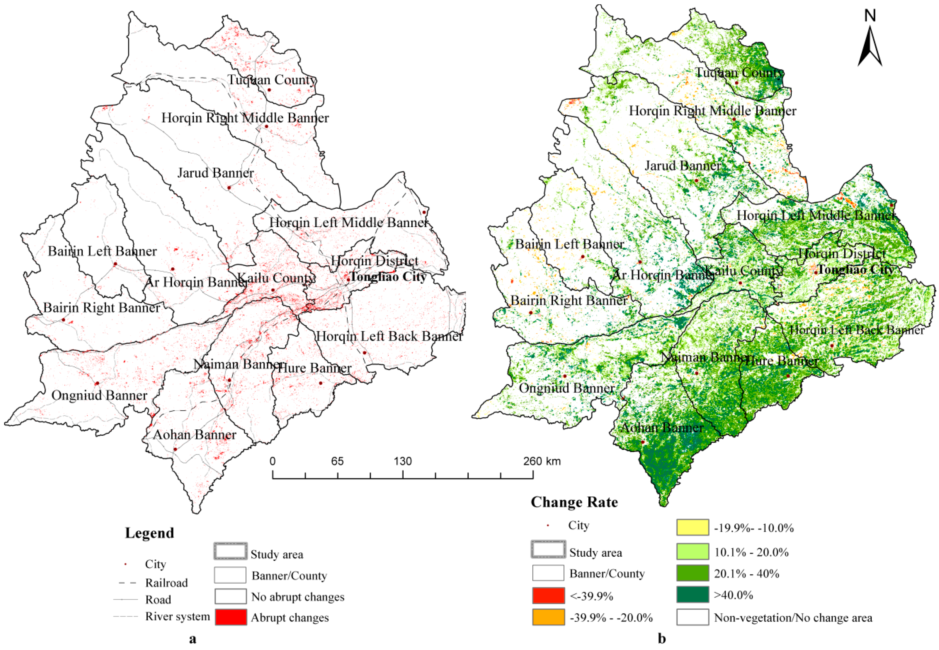
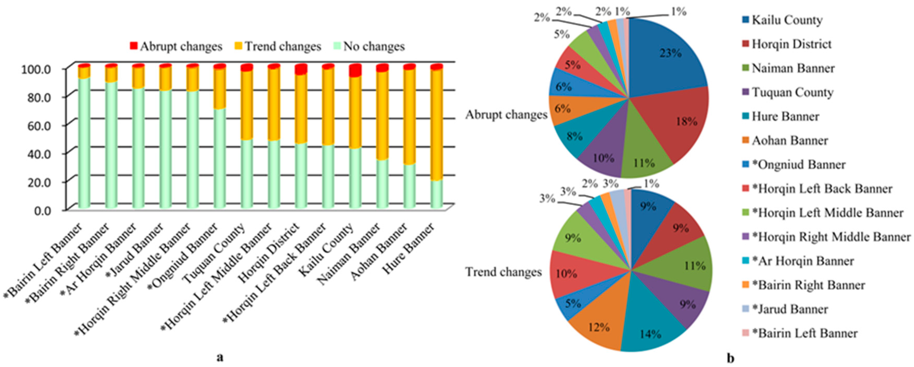
3.1. Land Cover Changes
3.2. Accuracy Assessment
3.2.1. Accuracies of Abrupt Land Cover Changes
3.2.2. Accuracies of Trend Land Cover Changes
4. Discussion
4.1. Improvement of MTHD Method
4.2. Errors of Abrupt Land Cover Changes
4.3. Limitations and Further Research
4.3.1. Limitations in Detecting Abrupt Land Cover Changes
4.3.2. Limitation of Data Sources
4.3.3. Other Uncertainties
5. Conclusions
Acknowledgments
Author Contributions
Conflicts of Interest
References
- Lu, D.; Mausel, P.; Brondizio, E.; Moran, E. Change detection techniques. Int. J. Remote Sens. 2004, 25, 2365–2401. [Google Scholar] [CrossRef]
- Hobbs, R.J. Remote sensing of spatial and temporal dynamics of vegetation. In Remote Sensing of Biosphere Functioning, 1st ed.; Hobbs, R.J., Mooney, H.A., Eds.; Springer-Verlag: New York, NY, USA, 1990; pp. 203–219. [Google Scholar]
- Scheffer, M.; Carpenter, S.; Foley, J.A.; Folke, C.; Walker, B. Catastrophic shifts in ecosystems. Nature 2001, 413, 591–596. [Google Scholar] [CrossRef] [PubMed]
- Kennedy, R.E.; Andrefouet, S.; Cohen, W.B.; Gomez, C.; Griffiths, P.; Hais, M.; Healey, S.P.; Helmer, E.H.; Hostert, P.; Lyons, M.B.; et al. Bringing an ecological view of change to Landsat-based remote sensing. Front. Ecol. Environ. 2014, 12, 339–346. [Google Scholar] [CrossRef]
- Lambin, E.F.; Geist, H.J. Land-Use and Land-Cover Change: Local Processes and Global Impacts; Springer: Berlin, Germany, 2006; pp. 33–39. [Google Scholar]
- Lu, D.; Li, G.; Moran, E. Current situation and needs of change detection techniques. Int. J. Image Data Fusion 2014, 5, 13–38. [Google Scholar] [CrossRef]
- Verbesselt, J.; Zeileis, A.; Herold, M. Near real-time disturbance detection using satellite image time series. Remote Sens. Environ. 2012, 123, 98–108. [Google Scholar] [CrossRef]
- Jin, S.; Sader, S.A. MODIS time-series imagery for forest disturbance detection and quantification of patch size effects. Remote Sens. Environ. 2005, 99, 462–470. [Google Scholar] [CrossRef]
- De Jong, R.; Verbesselt, J.; Zeileis, A.; Schaepman, M.E. Shifts in global vegetation activity trends. Remote Sens. 2013, 5, 1117–1133. [Google Scholar] [CrossRef]
- Zhou, Q.M.; Li, B.L.; Chen, Y.M. Remote sensing change detection and process analysis of long-term land use change and human impacts. Ambio 2011, 40, 807–818. [Google Scholar] [CrossRef] [PubMed]
- Dubinin, M.; Luschekina, A.; Radeloff, V.C. Climate, livestock, and vegetation: What drives fire increase in the arid ecosystems of southern Russia? Ecosystems 2011, 14, 547–562. [Google Scholar] [CrossRef]
- De Jong, R.; de Bruin, S.; de Wit, A.; Schaepman, M.E.; Dent, D.L. Analysis of monotonic greening and browning trends from global NDVI time-series. Remote Sens. Environ. 2011, 115, 692–702. [Google Scholar] [CrossRef]
- Forkel, M.; Carvalhais, N.; Verbesselt, J.; Mahecha, M.D.; Neigh, C.S.; Reichstein, M. Trend change detection in NDVI time series: Effects of inter-annual variability and methodology. Remote Sens. 2013, 5, 2113–2144. [Google Scholar] [CrossRef]
- Eckert, S.; Hüsler, F.; Liniger, H.; Hodel, E. Trend analysis of MODIS NDVI time series for detecting land degradation and regeneration in Mongolia. J. Arid Environ. 2015, 113, 16–28. [Google Scholar] [CrossRef]
- Coppin, P.; Jonckheere, I.; Nackaerts, K.; Muys, B.; Lambin, E. Review Article Digital change detection methods in ecosystem monitoring: A review. Int. J. Remote Sens. 2004, 25, 1565–1596. [Google Scholar] [CrossRef]
- Singh, A. Review article digital change detection techniques using remotely-sensed data. Int. J. Remote Sens. 1989, 10, 989–1003. [Google Scholar] [CrossRef]
- Kennedy, R.E.; Cohen, W.B.; Schroeder, T.A. Trajectory-based change detection for automated characterization of forest disturbance dynamics. Remote Sens. Environ. 2007, 110, 370–386. [Google Scholar] [CrossRef]
- Zhu, Z.; Woodcock, C.E. Continuous change detection and classification of land cover using all available Landsat data. Remote Sens. Environ. 2014, 144, 152–171. [Google Scholar] [CrossRef]
- Cohen, W.B.; Yang, Z.; Kennedy, R. Detecting trends in forest disturbance and recovery using yearly Landsat time series: 2. TimeSync—Tools for calibration and validation. Remote Sens. Environ. 2010, 114, 2911–2924. [Google Scholar] [CrossRef]
- Kennedy, R.E.; Yang, Z.; Cohen, W.B. Detecting trends in forest disturbance and recovery using yearly Landsat time series: 1. LandTrendr—Temporal segmentation algorithms. Remote Sens. Environ. 2010, 114, 2897–2910. [Google Scholar] [CrossRef]
- Piao, S.L.; Wang, X.; Ciais, P.; Zhu, B.; Wang, T.; Liu, J. Changes in satellite-derived vegetation growth trend in temperate and boreal Eurasia from 1982 to 2006. Glob. Chang. Biol. 2011, 17, 3228–3239. [Google Scholar] [CrossRef]
- Adosi, J.J. Seasonal variation of carbon dioxide, rainfall, NDVI and it’s association to land degradation in Tanzania. In Climate and Land Degradation; Sivakumar, M.V., Ndiang’Ui, N., Eds.; Springer: Berlin/Heidelberg, Germany, 2007; pp. 373–389. [Google Scholar]
- Li, Z.; Huffman, T.; McConkey, B.; Townley-Smith, L. Monitoring and modeling spatial and temporal patterns of grassland dynamics using time-series MODIS NDVI with climate and stocking data. Remote Sens. Environ. 2013, 138, 232–244. [Google Scholar] [CrossRef]
- Geerken, R.A. An algorithm to classify and monitor seasonal variations in vegetation phenologies and their inter-annual change. ISPRS J. Photogramm. 2009, 64, 422–431. [Google Scholar] [CrossRef]
- Olsson, L.; Eklundh, L.; Ardö, J. A recent greening of the Sahel-trends, patterns and potential causes. J. Arid Environ. 2005, 63, 556–566. [Google Scholar] [CrossRef]
- Evans, J.; Geerken, R. Discrimination between climate and human-induced dryland degradation. J. Arid Environ. 2004, 57, 535–554. [Google Scholar] [CrossRef]
- Ahmedou, O.; Nagasawa, R.; Osman, A.; Hattori, K. Rainfall variability and vegetation dynamics in the Mauritanian Sahel. Clim. Res. 2009, 38, 75–81. [Google Scholar] [CrossRef]
- Potter, C.; Tan, P.N.; Steinbach, M.; Klooster, S.; Kumar, V.; Myneni, R.; Genovese, V. Major disturbance events in terrestrial ecosystems detected using global satellite data sets. Glob. Chang. Biol. 2003, 9, 1005–1021. [Google Scholar] [CrossRef]
- Xue, Y.; Liu, S.; Zhang, L.; Hu, Y. Integrating fuzzy logic with piecewise linear regression for detecting vegetation greenness change in the Yukon River Basin, Alaska. Int. J. Remote Sens. 2013, 34, 4242–4263. [Google Scholar] [CrossRef]
- Gao, Q.Z.; Li, Y.; Wan, Y.F.; Zhang, W.N.; Borjigdai, A. Challenges in disentangling the influence of climatic and socio-economic factors on alpine grassland ecosystems in the source area of Asian major rivers. Quatern. Int. 2013, 304, 126–132. [Google Scholar]
- Wessels, K.; Prince, S.; Malherbe, J.; Small, J.; Frost, P.; VanZyl, D. Can human-induced land degradation be distinguished from the effects of rainfall variability? A case study in South Africa. J. Arid Environ. 2007, 68, 271–297. [Google Scholar] [CrossRef]
- Jamali, S.; Jönsson, P.; Eklundh, L.; Ardö, J.; Seaquist, J. Detecting changes in vegetation trends using time series segmentation. Remote Sens. Environ. 2015, 156, 182–195. [Google Scholar] [CrossRef]
- Verbesselt, J.; Hyndman, R.; Zeileis, A.; Culvenor, D. Phenological change detection while accounting for abrupt and gradual trends in satellite image time series. Remote Sens. Environ. 2010, 114, 2970–2980. [Google Scholar] [CrossRef]
- Verbesselt, J.; Hyndman, R.; Newnham, G.; Culvenor, D. Detecting trend and seasonal changes in satellite image time series. Remote Sens. Environ. 2010, 114, 106–115. [Google Scholar] [CrossRef]
- Bai, J.; Perron, P. Computation and analysis of multiple structural change models. J. Appl. Econ. 2003, 18, 1–22. [Google Scholar] [CrossRef]
- Brown, M.B.; Forsythe, A.B. The small sample behavior of some statistics which test the equality of several means. Technometrics 1974, 16, 129–132. [Google Scholar] [CrossRef]
- Brown, M.B.; Forsythe, A.B. Robust tests for the equality of variances. J. Am. Stat. Assoc. 1974, 69, 364–367. [Google Scholar] [CrossRef]
- Tomé, A.; Miranda, P. Piecewise linear fitting and trend changing points of climate parameters. Geophys. Res. Lett. 2004, 31, L02207. [Google Scholar] [CrossRef]
- Tomé, A.; Miranda, P. Continuous partial trends and low-frequency oscillations of time series. Nonlinear Proc. Geophys. 2005, 12, 451–460. [Google Scholar] [CrossRef]
- Toyoda, T. Use of the chow test under heteroscedasticity. Econometrica 1974, 42, 601–608. [Google Scholar] [CrossRef]
- Huang, F.; Wang, P.; Liu, X.N. Monitoring vegetation dynamic in Horqin sandy land from spot vegetation time series imagery. Int. Arch. Photogramm. Remote Sens. Spat. Inf. Sci. 2008, 37, 915–920. [Google Scholar]
- Lu, D.; Neilson, W.A. (Eds.) China’s West Region Development—Domestic Strategies and Global Implications; World Scientific Publishing Co. Pte. Ltd.: Singapore, Singapore, 2004; pp. 191–193.
- Feng, Z.M.; Yang, Y.Z.; Zhang, Y.Q.; Zhang, P.T.; Li, Y.Q. Grain-for-green policy and its impacts on grain supply in West China. Land Use Policy 2005, 22, 301–312. [Google Scholar] [CrossRef]
- Wu, Z.T.; Wu, J.J.; He, B.; Liu, J.H.; Wang, Q.F.; Zhang, H. Drought offset ecological restoration program-induced increase in vegetation activity in the Beijing–Tianjin Sand Source Region, China. Environ. Sci. Technol. 2014, 48, 12108–12117. [Google Scholar] [CrossRef] [PubMed]
- Yan, Q.L.; Zhu, J.J.; Hu, Z.B.; Sun, O.J. Environmental impacts of the shelter forests in Horqin Sandy Land, Northeast China. J. Environ. Qual. 2011, 40, 815–824. [Google Scholar] [CrossRef] [PubMed]
- Zhang, G.; Dong, J.; Xiao, X.; Hu, Z.; Sheldon, S. Effectiveness of ecological restoration projects in Horqin Sandy Land, China based on SPOT-VGT NDVI data. Ecol. Eng. 2012, 38, 20–29. [Google Scholar] [CrossRef]
- Han, Z.; Wang, T.; Yan, C.; Liu, Y.; Liu, L.; Li, A.; Du, H. Change trends for desertified lands in the Horqin Sandy Land at the beginning of the twenty-first century. Environ. Earth Sci. 2010, 59, 1749–1757. [Google Scholar] [CrossRef]
- Yan, Q.; Zhu, J.; Zheng, X.; Jin, C. Causal effects of shelter forests and water factors on desertification control during 2000–2010 at the Horqin Sandy Land region, China. J. For. Res. 2015, 26, 33–45. [Google Scholar] [CrossRef]
- Petit, C.; Scudder, T.; Lambin, E. Quantifying processes of land-cover change by remote sensing: Resettlement and rapid land-cover changes in south-eastern Zambia. Int. J. Remote Sens. 2001, 22, 3435–3456. [Google Scholar] [CrossRef]
- Xu, L.L.; Li, B.L.; Yuan, Y.C.; Gao, X.Z.; Zhang, T. A Temporal-spatial iteration method to reconstruct NDVI time series datasets. Remote Sens. 2015, 7, 8906–8924. [Google Scholar] [CrossRef]
- Tian, F.; Fensholt, R.; Verbesselt, J.; Grogan, K.; Horion, S.; Wang, Y.J. Evaluating temporal consistency of long-term global NDVI datasets for trend analysis. Remote Sens. Environ. 2015, 163, 326–340. [Google Scholar] [CrossRef]
- Lyon, J.G.; Yuan, D.; Lunetta, R.S.; Elvidge, C.D. A change detection experiment using vegetation indices. Photogramm. Eng. Remote Sens. 1998, 64, 143–150. [Google Scholar]
- Lunetta, R.S.; Knight, J.F.; Ediriwickrema, J.; Lyon, J.G.; Worthy, L.D. Land-cover change detection using multi-temporal MODIS NDVI data. Remote Sens. Environ. 2006, 105, 142–154. [Google Scholar] [CrossRef]
- Young, S.S.; Wang, C.Y. Land-cover change analysis of China using global-scale Pathfinder AVHRR Land cover (PAL) data, 1982–92. Int. J. Remote Sens. 2001, 22, 1457–1477. [Google Scholar]
- Index of /MOLT. Available online: http://e4ftl01.cr.usgs.gov/MOLT/ (accessed on 1 May 2013).
- Savitzky, A.; Golay, M.J. Smoothing and differentiation of data by simplified least squares procedures. Anal. Chem. 1964, 36, 1627–1639. [Google Scholar] [CrossRef]
- Chen, J.; Jönsson, P.; Tamura, M.; Gu, Z.; Matsushita, B.; Eklundh, L. A simple method for reconstructing a high-quality NDVI time-series data set based on the Savitzky-Golay filter. Remote Sens. Environ. 2004, 91, 332–344. [Google Scholar] [CrossRef]
- Fang, J.Y.; Piao, S.L.; He, J.S.; Ma, W.H. Increasing terrestrial vegetation activity in China, 1982–1999. Sci. China C Life Sci. 2004, 47, 229–240. [Google Scholar] [PubMed]
- USGS Global Visualization Viewer. Available online: http://glovis.usgs.gov/ (accessed on 20 March 2014).
- Lee, D.S.; Storey, J.C.; Choate, M.J.; Hayes, R.W. Four years of Landsat-7 on-orbit geometric calibration and performance. IEEE Trans. Geosci. Remote Sens. 2004, 42, 2786–2795. [Google Scholar] [CrossRef]
- Gitelson, A.A.; Peng, Y.; Masek, J.G.; Rundquist, D.C.; Verma, S.; Suyker, A.; Baker, J.M.; Hatfield, J.L.; Meyers, T. Remote estimation of crop gross primary production with Landsat data. Remote Sens. Environ. 2012, 121, 404–414. [Google Scholar] [CrossRef]
- Scepan, J.; Menz, G.; Hansen, M.C. The DISCover validation image interpretation process. Photogramm. Eng. Remote Sens. 1999, 65, 1075–1081. [Google Scholar]
- Potapov, P.; Hansen, M.C.; Stehman, S.V.; Loveland, T.R.; Pittman, K. Combining MODIS and Landsat imagery to estimate and map boreal forest cover loss. Remote Sens. Environ. 2008, 112, 3708–3719. [Google Scholar] [CrossRef]
- Xu, L.L.; Li, B.L.; Yuan, Y.C.; Gao, X.Z.; Liu, H.J.; Dong, G.H. Changes in China’s cultivated land and the evaluation of land requisition-compensation balance policy from 2000 to 2010. Resour. Sci. 2015, 37, 1543–1551. [Google Scholar]
- Grubbs, F.E. Sample criteria for testing outlying observations. Ann. Math. Stat. 1950, 21, 27–58. [Google Scholar] [CrossRef]
- Zhang, Y.C.; Zhou, C.H.; Li, B.L. Brown-Forsythe based method for detecting change points in hydrological time series. Geogr. Res. 2005, 24, 741–748. [Google Scholar]
- De Beurs, K.; Henebry, G. A statistical framework for the analysis of long image time series. Int. J. Remote Sens. 2005, 26, 1551–1573. [Google Scholar] [CrossRef]
- Hall, F.G.; Strebel, D.E.; Nickeson, J.E.; Goetz, S.J. Radiometric rectification: Toward a common radiometric response among multidate, multisensor images. Remote Sens. Environ. 1991, 35, 11–27. [Google Scholar] [CrossRef]
- Labus, M.P.; Nielsen, G.A.; Lawrence, R.L.; Long, D.S. Wheat yield estimates using multi-temporal NDVI satellite imagery. Int. J. Remote Sens. 2002, 23, 4169–4180. [Google Scholar] [CrossRef]
- Pontius, R.G.; Shusas, E.; McEachern, M. Detecting important categorical land changes while accounting for persistence. Agric. Ecosyst. Environ. 2004, 101, 251–268. [Google Scholar] [CrossRef]
- Yuan, Y.C.; Li, B.L.; Gao, X.Z.; Liu, H.J.; Xu, L.L.; Zhou, C.H. A method of characterizing land-cover swap changes in the arid zone of China. Front. Earth Sci. 2016, 10, 74–86. [Google Scholar] [CrossRef]
- Drusch, M.; del Bello, U.; Carlier, S.; Colin, O.; Fernandez, V.; Gascon, F.; Hoersch, B.; Isola, C.; Laberinti, P.; Martimort, P. Sentinel-2: ESA’s optical high-resolution mission for GMES operational services. Remote Sens. Environ. 2012, 120, 25–36. [Google Scholar] [CrossRef]


| PATH/ROW | Period 1 | Period 2 | Period 3 |
|---|---|---|---|
| 122/28 | 21 August 2000 (LT5) | 4 September 2005 (LT5) | 1 August 2010 (LT5) |
| 122/29 | 6 September 2000 (LT5) | 22 August 2006 (LT5) | 18 September 2010 (LT5) |
| 122/30 | 6 September 2000 (LT5) | 4 September 2005 (LT5) | 1 August 2010 (LT5) |
| 123/29 | 28 June 2001 (LT5) | 29 August 2006 (LT5) | 24 August 2010 (LT5) |
| 121/28 | 13 July 2000 LT5) | 31 August 2006 (LT5) | 10 August 2010 (LT5) |
| 121/29 | 14 August 2000 (LT5) | 16 September 2006 (LT5) | 10 August 2010 (LT5) |
| 121/30 | 14 August 2000 (LT5) | 16 September 2006 (LT5) | 10 August 2010 (LT5) |
| 121/31 | 7 September 2000 (LE7) | 16 September 2006 (LT5) | 10 August 2010 (LT5) |
| 120/29 | 10 August 2001 (LT5) | 6 September 2005 (LT5) | 22 August 2011 (LT5) |
| 120/30 | 24 September 2000 (LT5) | 5 September 2005 (LT5) | 17 August 2009 (LT5) |
| Abrupt Change | Trend Change | No Change | |
|---|---|---|---|
| Area (km2) | 2176.3 | 44,574.9 | 83,638.7 |
| Percentage (%) | 1.7% | 34.2 | 64.1 |
| Change Rate | Cropland | Grassland | Woodland | Wetland | Built-Up Area | Unused Land | Total | |
|---|---|---|---|---|---|---|---|---|
| >40 | km2 | 4496.6 | 3044.3 | 1246.7 | 181.6 | 148.6 | 539.8 | 9657.6 |
| % | 10.1 | 6.8 | 2.8 | 0.4 | 0.3 | 1.2 | 21.7 | |
| 20–40 | km2 | 11,959.6 | 8139.9 | 1691.7 | 214.5 | 585.5 | 981.6 | 23,572.8 |
| % | 26.8 | 18.3 | 3.8 | 0.5 | 1.3 | 2.2 | 2.9 | |
| 10–20 | km2 | 4600.4 | 2936.5 | 596.8 | 74.3 | 384.5 | 639.3 | 9231.8 |
| % | 10.3 | 6.6 | 1.3 | 0.2 | 0.9 | 1.4 | 20.7 | |
| −10–−20 | km2 | 163.1 | 433.4 | 117.0 | 20.1 | 40.6 | 154.2 | 928.4 |
| % | 0.4 | 1.0 | 0.3 | 0.0 | 0.1 | 0.3 | 2.1 | |
| −20–−40 | km2 | 96.2 | 530.6 | 62.0 | 52.0 | 51.9 | 219.2 | 1011.9 |
| % | 0.2 | 1.2 | 0.1 | 0.1 | 0.1 | 0.5 | 2.3 | |
| <−40 | km2 | 21.0 | 56.0 | 2.8 | 46.5 | 21.2 | 24.9 | 172.4 |
| % | 0.0 | 0.1 | 0.0 | 0.1 | 0.0 | 0.1 | 0.3 | |
| Total | km2 | 21,336.9 | 15,140.7 | 3717.1 | 588.9 | 1232.3 | 2559.0 | 44,574.9 |
| % | 47.9 | 34.0 | 8.3 | 1.3 | 2.8 | 5.7 | 100 | |
| Reference | ||||||
|---|---|---|---|---|---|---|
| Abrupt Changes | No Abrupt Changes | Total | User’s Accuracy | Commission Error | ||
| Classified | Abrupt changes | 80 | 20 | 100 | 80.0% | 20.0% |
| No abrupt changes | 6 | 94 | 100 | 94.0% | 6.0% | |
| Total | 86 | 114 | 200 | |||
| Producer’s accuracy | 93.0% | 82.5% | Overall accuracy = 87.0% | |||
| Omission error | 7.0% | 17.5% | Kappa index = 0.74 | |||
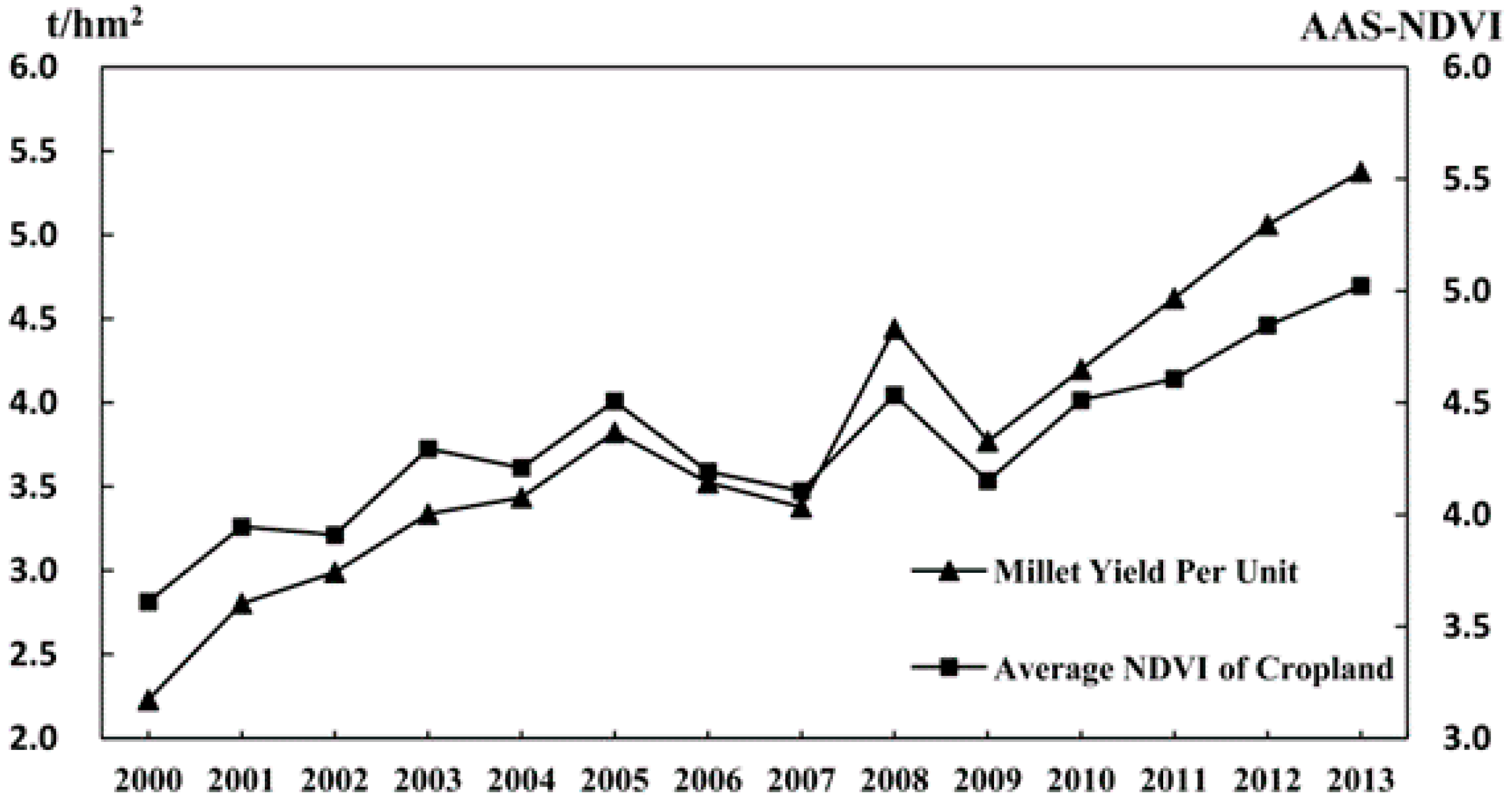
| Statistical Area | Equation of Linear Regression | R2 | p |
|---|---|---|---|
| Tuquan County | y = 0.31x + 3.21 | 0.66 | p < 0.01 |
| Horqin Right Middle Banner * | y = 0.26x + 3.59 | 0.55 | p < 0.01 |
| Jarud Banner * | y = 0.46x + 2.96 | 0.46 | p < 0.01 |
| Ar Horqin Banner * | y = 0.47x + 3.27 | 0.79 | p < 0.01 |
| Horqin Left Middle Banner * | y = 0.16x + 3.54 | 0.79 | p < 0.01 |
| Bairin Left Banner * | y = 0.43x + 3.58 | 0.73 | p < 0.01 |
| Bairin Right Banner * | y = 0.16x + 3.91 | 0.13 | p = 0.20 |
| Kailu County | y = 0.36x + 2.25 | 0.86 | p < 0.01 |
| Horqin District | y = 0.70x + 0.49 | 0.55 | p < 0.01 |
| Horqin Left Back Banner * | y = 0.47x + 2.73 | 0.69 | p < 0.01 |
| Naiman Banner | y = 0.35x + 2.93 | 0.69 | p < 0.01 |
| Ongniud Banner * | y = 0.40x + 2.57 | 0.70 | p < 0.01 |
| Hure Banner | y = 0.25x + 3.21 | 0.78 | p < 0.01 |
| Aohan Banner | y = 0.43x + 2.88 | 0.72 | p < 0.01 |
| The whole study area | y = 0.42x + 2.72 | 0.94 | p < 0.01 |
| Error | Error Sources | Samples | Graphical Representation (from → to) | Descriptions for Graphical Representation | |
|---|---|---|---|---|---|
| Amount | Percentage | ||||
| Commission | Limited land cover changes | 11 | 55.0% | 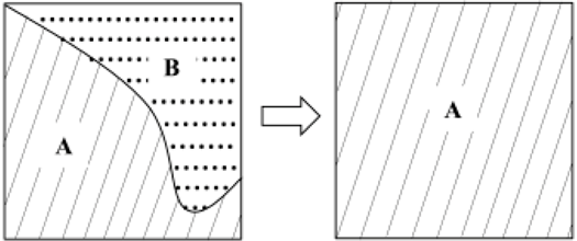 | A mixed pixel with type A and B turned to a pixel with type A, less than 60% of land cover type changes in a pixel happened. |
| Changes of crop species in cropland | 9 | 45.0% | 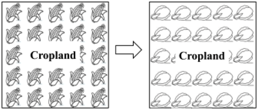 | Crop changed from corn to vegetable in a pixel. | |
| Omission | Counteracting spectral effects | 4 | 66.7% | 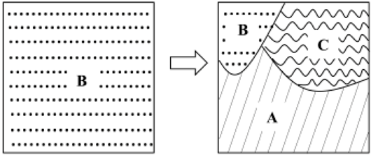 | A pixel with type B turn to a mixed pixel with type B, type A with high NDVIs and C with low NDVIs. |
| Swap changes | 2 | 33.3% |  | A mixed pixel with type A and B. While A and B were swap more than 60% to each other within the pixel. | |
© 2016 by the authors; licensee MDPI, Basel, Switzerland. This article is an open access article distributed under the terms and conditions of the Creative Commons Attribution (CC-BY) license (http://creativecommons.org/licenses/by/4.0/).
Share and Cite
Xu, L.; Li, B.; Yuan, Y.; Gao, X.; Zhang, T.; Sun, Q. Detecting Different Types of Directional Land Cover Changes Using MODIS NDVI Time Series Dataset. Remote Sens. 2016, 8, 495. https://doi.org/10.3390/rs8060495
Xu L, Li B, Yuan Y, Gao X, Zhang T, Sun Q. Detecting Different Types of Directional Land Cover Changes Using MODIS NDVI Time Series Dataset. Remote Sensing. 2016; 8(6):495. https://doi.org/10.3390/rs8060495
Chicago/Turabian StyleXu, Lili, Baolin Li, Yecheng Yuan, Xizhang Gao, Tao Zhang, and Qingling Sun. 2016. "Detecting Different Types of Directional Land Cover Changes Using MODIS NDVI Time Series Dataset" Remote Sensing 8, no. 6: 495. https://doi.org/10.3390/rs8060495
APA StyleXu, L., Li, B., Yuan, Y., Gao, X., Zhang, T., & Sun, Q. (2016). Detecting Different Types of Directional Land Cover Changes Using MODIS NDVI Time Series Dataset. Remote Sensing, 8(6), 495. https://doi.org/10.3390/rs8060495